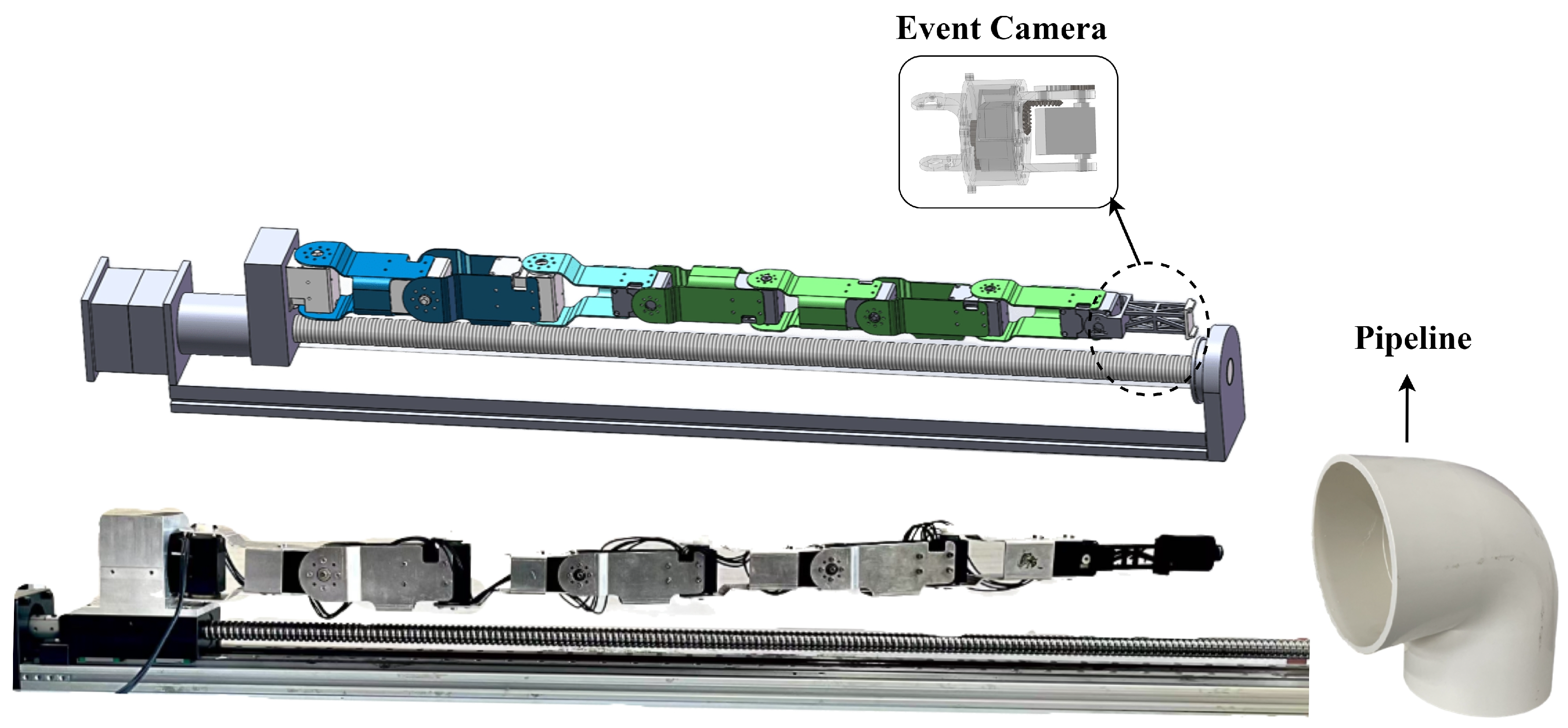
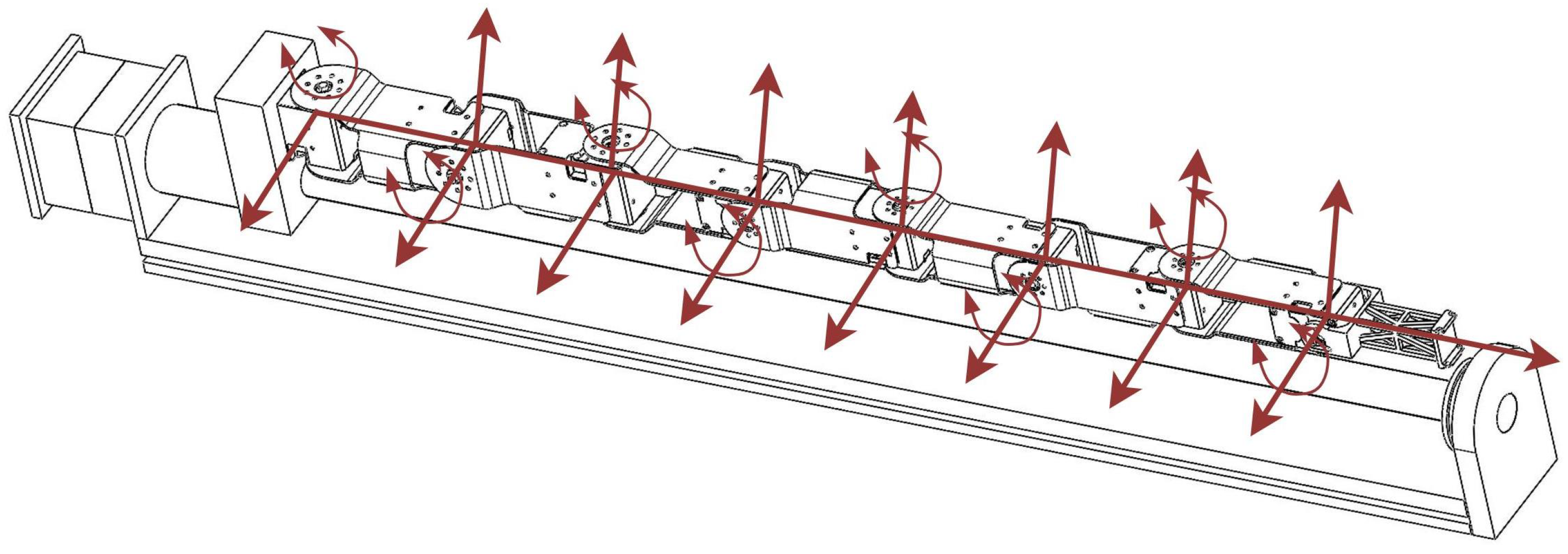
Figure 1.
Schematic diagram of the model of an HRM equipped with an event camera.
Figure 1.
Schematic diagram of the model of an HRM equipped with an event camera.
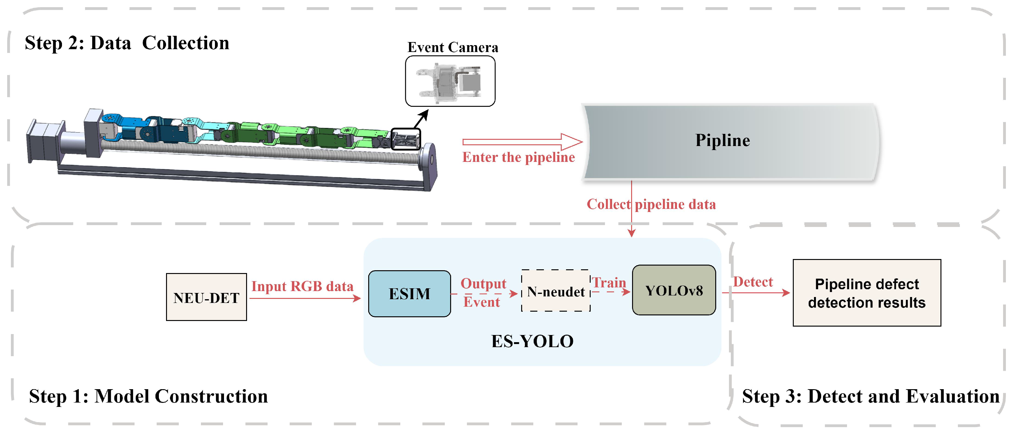
Figure 2.
Overall workflow of the pipeline defect detection method based on the ES-YOLO.
Figure 2.
Overall workflow of the pipeline defect detection method based on the ES-YOLO.
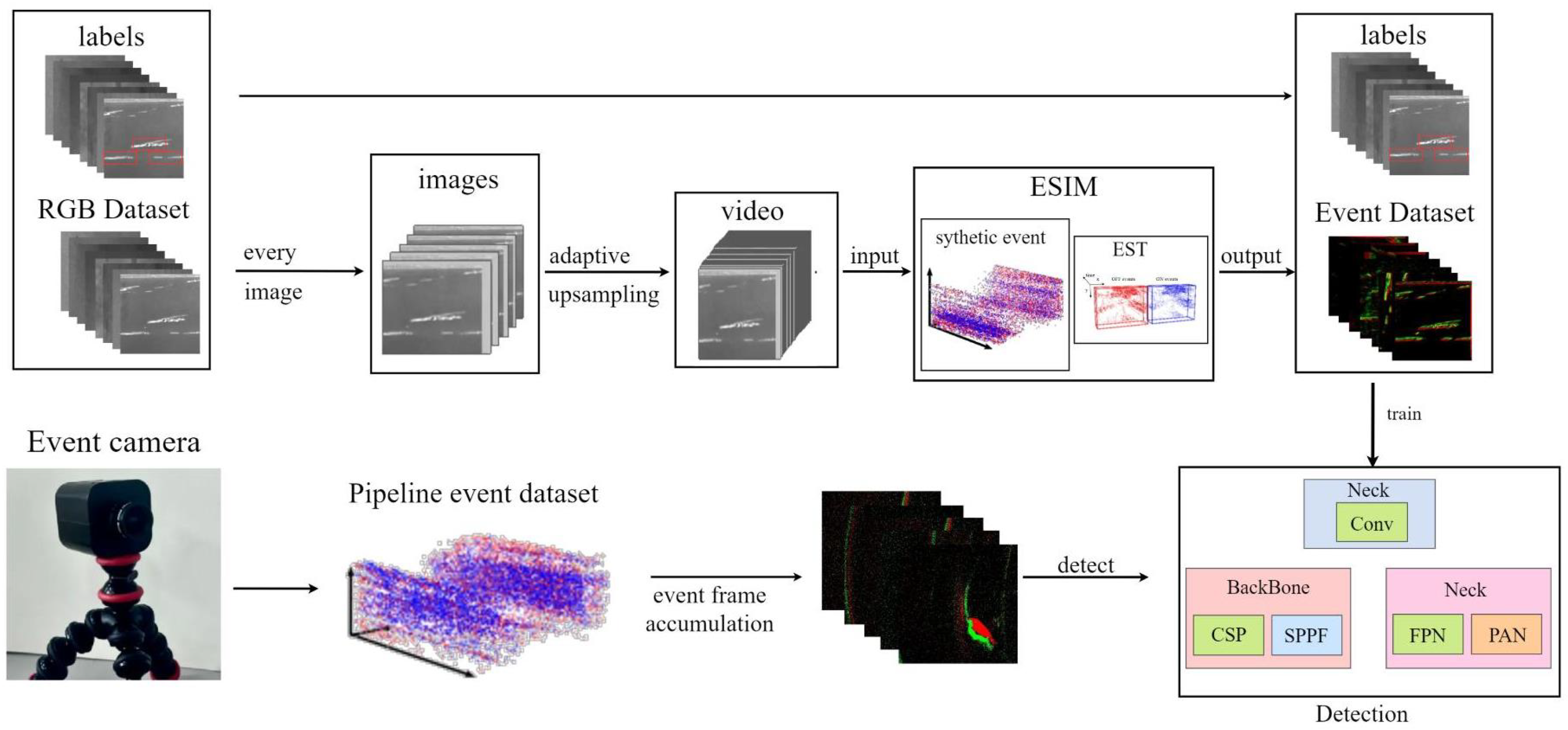
Figure 3.
ES-YOLO framework architecture. First, large-scale image datasets (NEU-DET) are converted into synthetic event datasets (N-neudet) through the ESIM module; then, the generated event data is passed to the YOLOv8 module for training.
Figure 3.
ES-YOLO framework architecture. First, large-scale image datasets (NEU-DET) are converted into synthetic event datasets (N-neudet) through the ESIM module; then, the generated event data is passed to the YOLOv8 module for training.
Figure 4.
Illustration of RGB dataset conversed into event dataset.
Figure 4.
Illustration of RGB dataset conversed into event dataset.
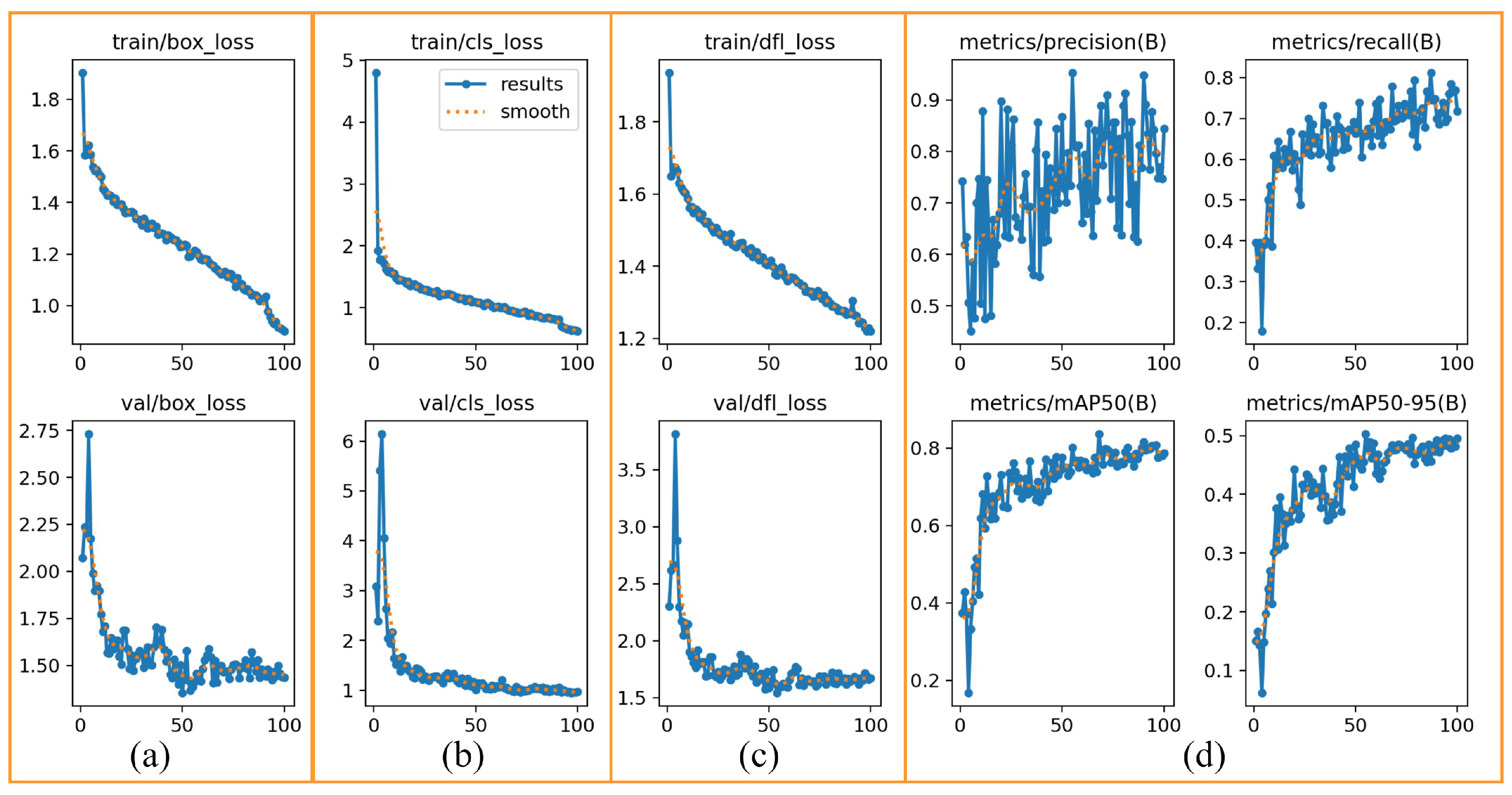
Figure 5.
Training result figures. (a) The bounding box loss (box_loss), which measures the error in predicted object locations, shows a consistent downward trend, indicating that the model is effectively learning to locate objects; (b) the classification loss (cls_loss), indicating the error in predicting the correct object class, also steadily decreases as training progresses; (c) Distribution Focal Loss (dfl_loss), another component for bounding box regression, follows a similar convergence pattern; (d) Key evaluation metrics, showing the progression of precision, recall, and mean Average Precision (mAP), all exhibit a clear upward trend, signifying significant performance improvement over time.
Figure 6.
Visualization of validation set results. (a) represents the ground truth; (b) represents the prediction results of the validation set.
Figure 6.
Visualization of validation set results. (a) represents the ground truth; (b) represents the prediction results of the validation set.
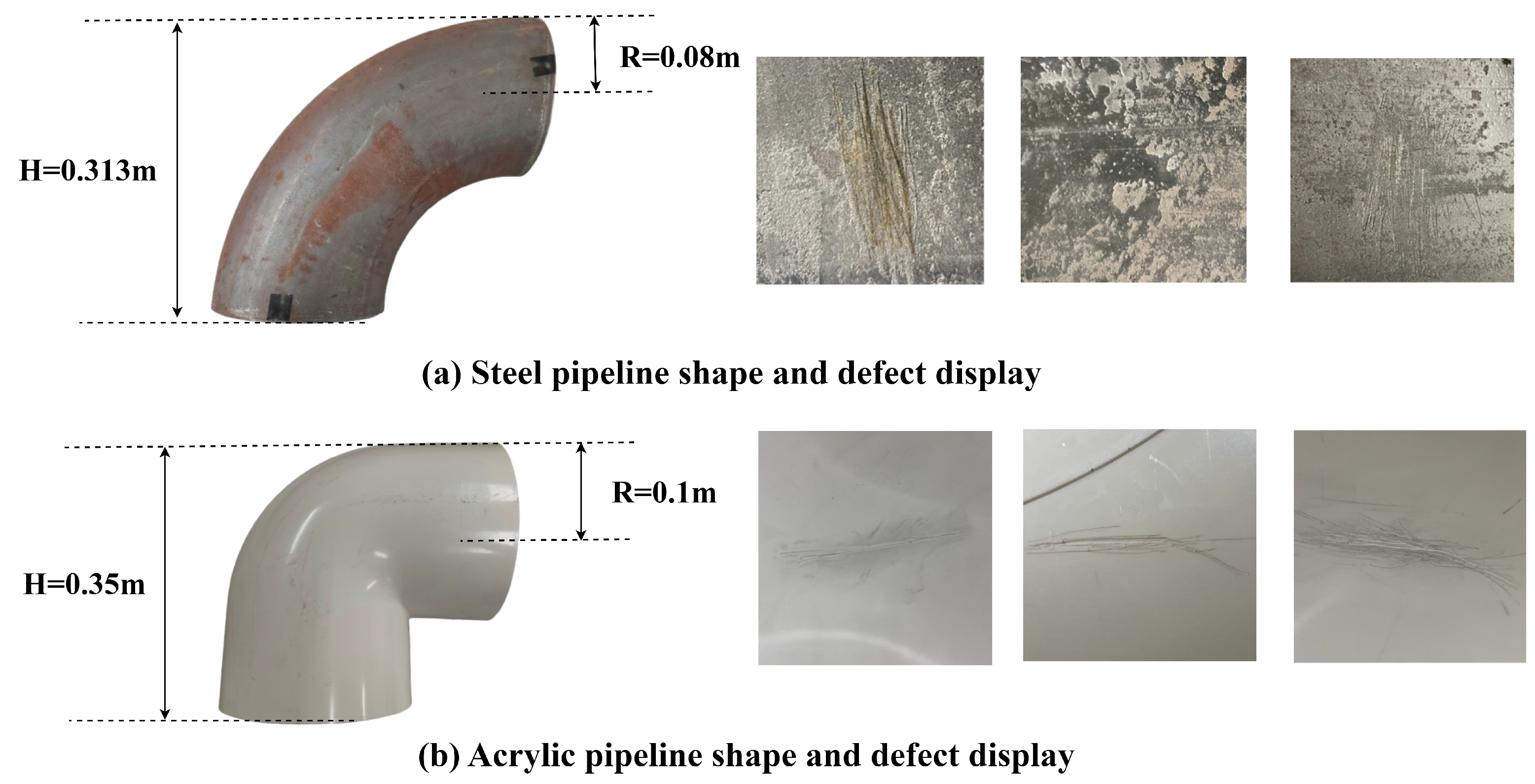
Figure 7.
Diagram showing the radius height of the experimental pipeline and its defects.
Figure 7.
Diagram showing the radius height of the experimental pipeline and its defects.
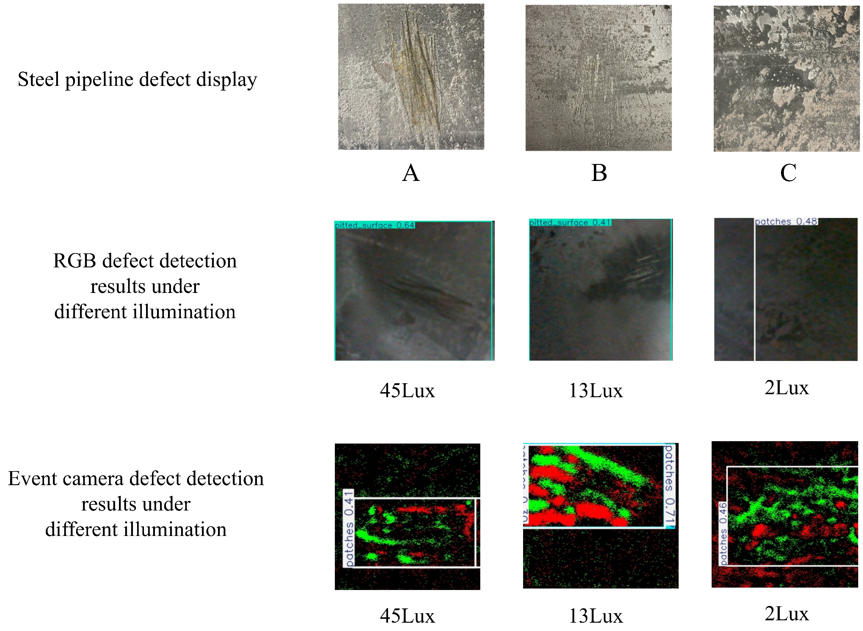
Figure 8.
Comparison experiment of different defects and illumination levels in steel pipes. Among them, A, B, and C represent the target defects in the steel pipe. Both the event camera and RGB camera can detect the defect at all three points (A, B, and C), where the illumination levels are 45 Lux, 13 Lux, and 2 Lux, respectively.
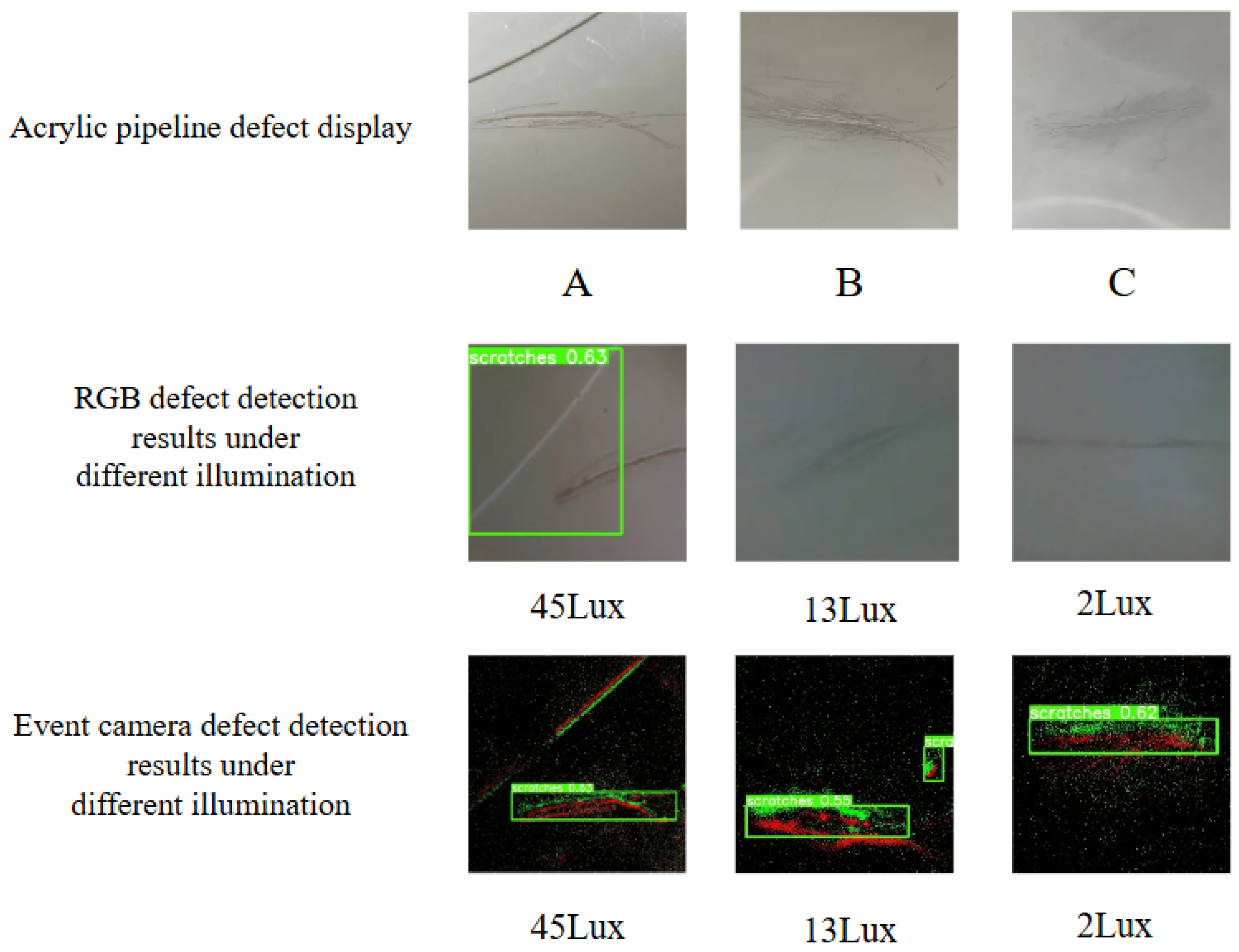
Figure 9.
Comparison experiment of different defects and illumination levels in acrylic pipes. Among them, A, B, and C represent the target defects in the acrylic pipe. The illumination levels are 13 Lux and 2 Lux when measured at points B and C, respectively. As a result, only the event camera successfully detected the defects.
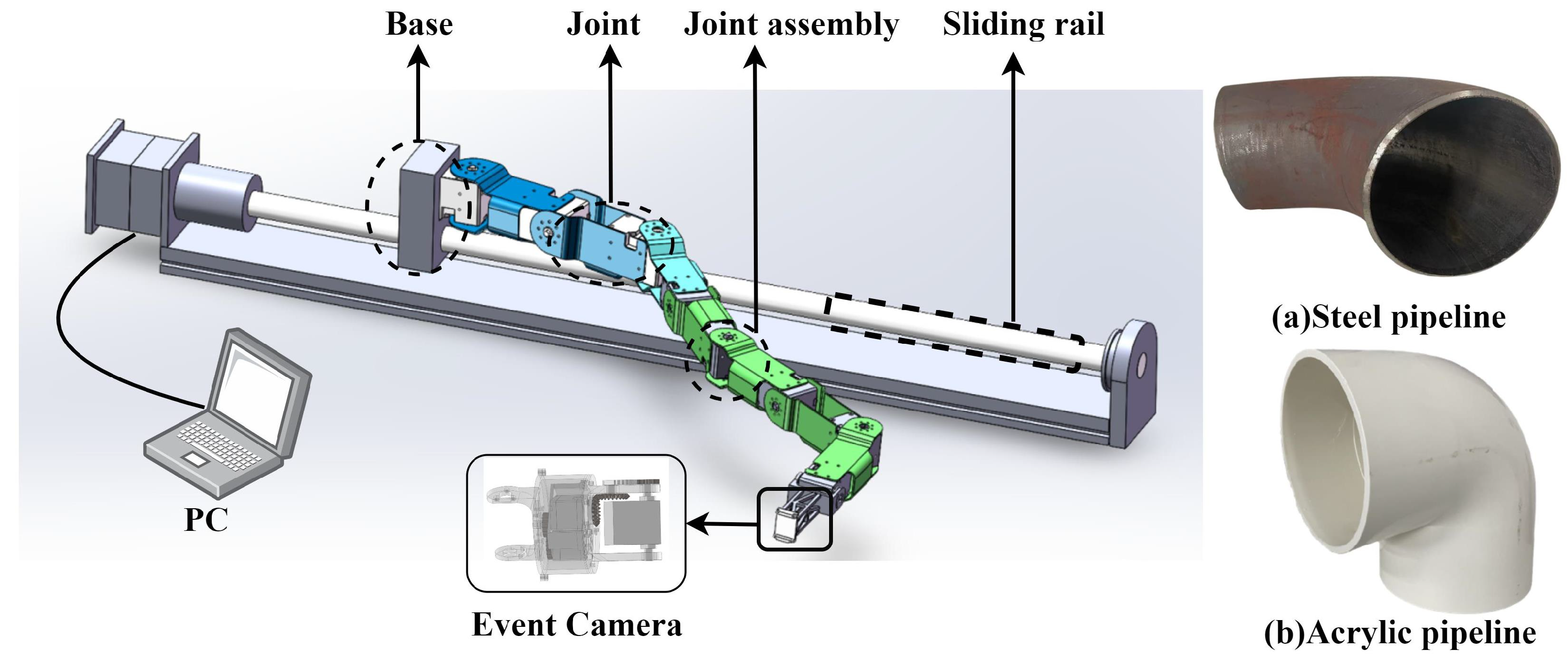
Figure 10.
Schematic diagram of the pipeline defect detection system, where (a) represents the steel pipeline and (b) corresponds to the acrylic pipeline.
Figure 10.
Schematic diagram of the pipeline defect detection system, where (a) represents the steel pipeline and (b) corresponds to the acrylic pipeline.
Figure 11.
Schematic diagram of the pipeline defect detection experimental workflow.
Figure 11.
Schematic diagram of the pipeline defect detection experimental workflow.
Figure 12.
Mechanical structure design of HRM and sliding rail.
Figure 12.
Mechanical structure design of HRM and sliding rail.
Figure 13.
Flow chart of the pipeline inspection process: (initial horizontal configuration), (collision-free configuration).
Figure 13.
Flow chart of the pipeline inspection process: (initial horizontal configuration), (collision-free configuration).
Figure 14.
Schematic diagram of single-bend pipe models with different curvatures, where the red solid line represents the pipeline centerline.
Figure 14.
Schematic diagram of single-bend pipe models with different curvatures, where the red solid line represents the pipeline centerline.
Figure 15.
Simulation results for the collision-free inspection of the pipeline defect detection system.
Figure 15.
Simulation results for the collision-free inspection of the pipeline defect detection system.
Figure 16.
Experimental platform for pipeline defect detection based on an event camera. The setup comprises the key components of the system, including a HRM, a movable base, a sliding rail, an event-based camera, and the pipeline specimen under inspection.
Figure 16.
Experimental platform for pipeline defect detection based on an event camera. The setup comprises the key components of the system, including a HRM, a movable base, a sliding rail, an event-based camera, and the pipeline specimen under inspection.
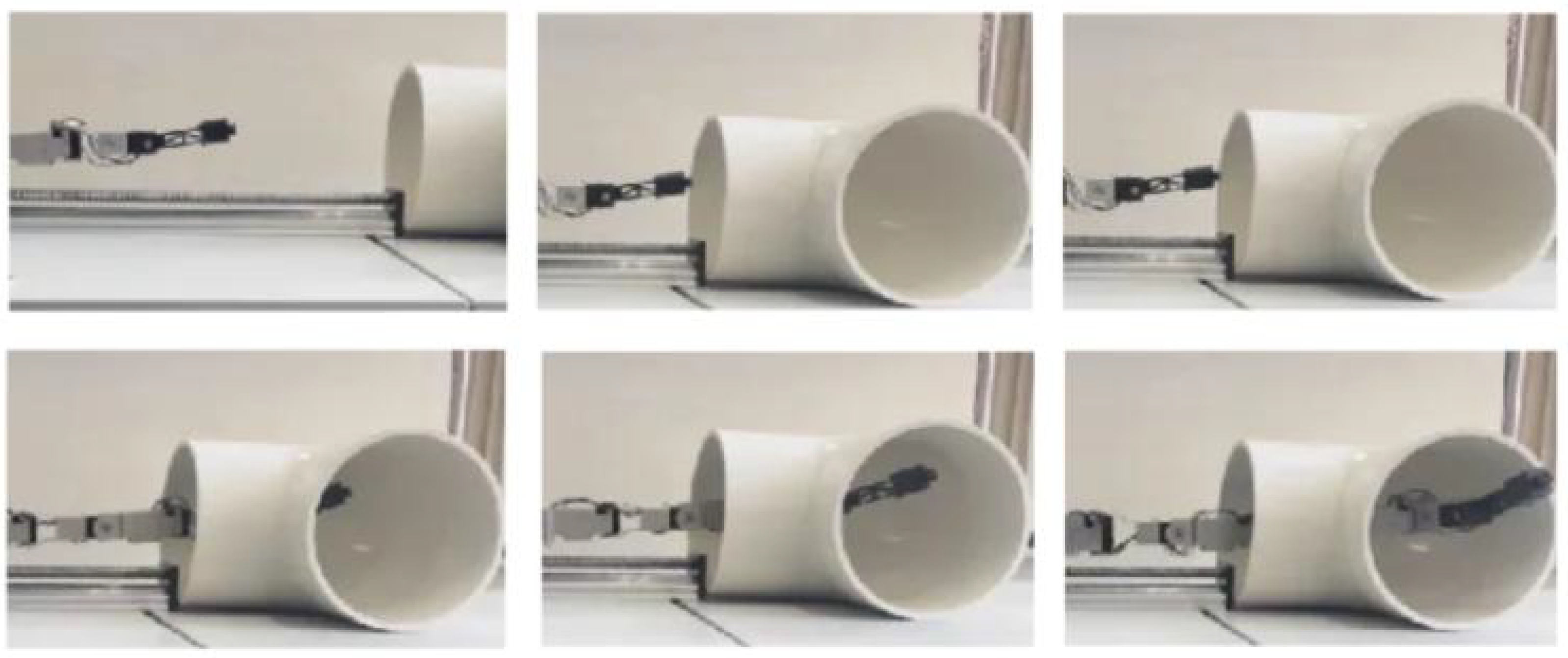
Figure 17.
The process of defect detection inside the pipeline using an event camera mounted on the HRM. Six consecutive frames illustrate the collision-free insertion of the HRM into the pipeline. The illuminance at the pipeline entrance is approximately 50 Lux. As the HRM advances deeper into the pipeline, occlusion of the entrance light source by its arm and its own shadow causes the light to diminish, with the minimum illuminance inside the pipeline dropping to approximately 10 Lux.
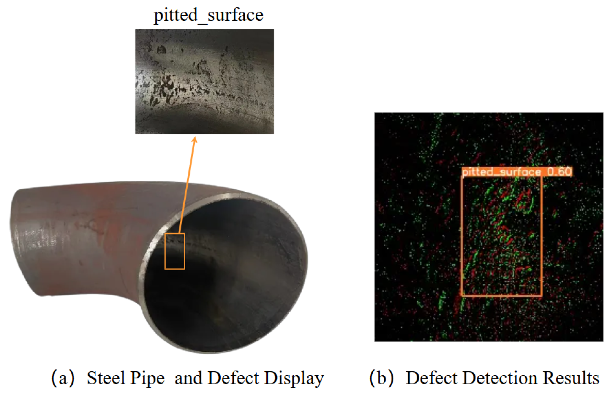
Figure 18.
Steel pipe internal defect detection. (a) shows the shape and defects of the steel pipe; (b) shows the detection results of the steel pipe.
Figure 18.
Steel pipe internal defect detection. (a) shows the shape and defects of the steel pipe; (b) shows the detection results of the steel pipe.
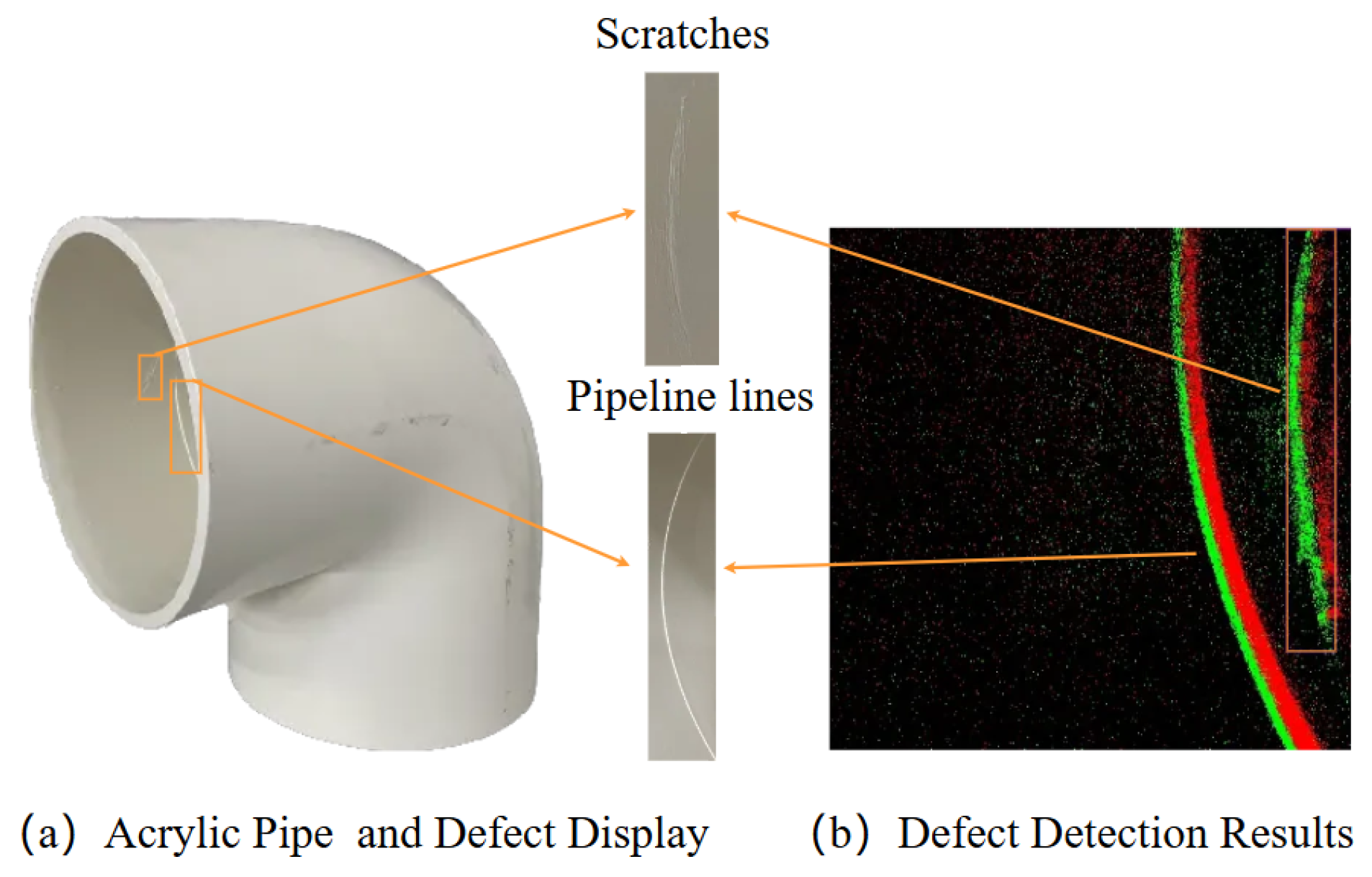
Figure 19.
Acrylic pipe internal defect detection. (a) shows the structure and defects of the acrylic pipe; (b) shows the detection results of the acrylic pipe defects.
Figure 19.
Acrylic pipe internal defect detection. (a) shows the structure and defects of the acrylic pipe; (b) shows the detection results of the acrylic pipe defects.
Table 1.
Training parameters.
Table 1.
Training parameters.
| Parameter | LR | Batch | Image | Monmentum | Epoch |
|---|
| Value | 0.01 | 64 | 640*640 | 0.937 | 100 |
Table 2.
ES-YOLO validating results.
Table 2.
ES-YOLO validating results.
| Class | P | R | mAP@0.5 | FNR | FDR |
|---|
| All | 0.952 | 0.657 | 0.801 | 0.343 | 0.048 |
| Crazing | 0.817 | 0.0714 | 0.238 | 0.9286 | 0.183 |
| Inclusion | 0.957 | 1 | 0.995 | 0 | 0.043 |
| Patches | 0.982 | 0.75 | 0.971 | 0.25 | 0.018 |
| Pitted | 1 | 0.62 | 0.876 | 0.38 | 0 |
| Rolled | 0.956 | 0.5 | 0.732 | 0.5 | 0.044 |
| Scratches | 0.998 | 1 | 0.995 | 0 | 0.002 |
Table 3.
Comparison of training results between RGB and event dataset.
Table 3.
Comparison of training results between RGB and event dataset.
| Framework | Dataset | P | R | mAP@0.5 | Inference Time |
|---|
| ES-YOLO | N-neudet | 0.952 | 0.657 | 0.801 | 79.167 ms |
| YOLO | NEU-DET | 0.84 | 0.637 | 0.773 | 69.444 ms |
Table 4.
Comparison results of event camera and RGB camera detection in steel pipes.
Table 4.
Comparison results of event camera and RGB camera detection in steel pipes.
| Target Defect | A | B | C |
|---|
| Illuminance | 45 Lux | 13 Lux | 2 Lux |
| Event camera | 94% | 90% | 84% |
| RGB camera | 66% | 30% | 10% |
Table 5.
Comparison results of event camera and RGB camera detection in acrylic pipes.
Table 5.
Comparison results of event camera and RGB camera detection in acrylic pipes.
| Target Defect | A | B | C |
|---|
| Illuminance | 45 Lux | 13 Lux | 2 Lux |
| Event camera | 82% | 76% | 68% |
| RGB camera | 34% | 10% | 0% |
Table 6.
Composition of the pipeline defect detection system.
Table 6.
Composition of the pipeline defect detection system.
| Component | Specifications |
|---|
| HRM | Three high-torque XH540-W270-R motors |
| Five lightweight XH430-W270-R motors |
| The sliding rail | Stepper motor |
| Lead screw |
| Base |
| Controller | PC(Intel(R) Core(TM) i5-8265U CPU @ 1.60GHz) |
| Protocol | RS485 protocol to control HRM |
| RS485 protocol to control sliding rail |
| Event camera | DVXplorer Mini |
Table 7.
D-H parameters of the snake manipulator.
Table 7.
D-H parameters of the snake manipulator.
| Link i | | | | |
|---|
| | | | 0 |
| | | | 0 |
Table 8.
Minimum safe passage radius of the HRM for different pipeline curvatures.
Table 8.
Minimum safe passage radius of the HRM for different pipeline curvatures.
| Curvatures | | | Minimum Pipeline Radius for Safe Passage |
|---|
| 4 cm | 2.53 cm | 6.53 cm |
| 4 cm | 3.72 cm | 7.72 cm |
| 4 cm | 5.13 cm | 9.13 cm |
Table 9.
Geometries of the two pipelines and experimental error results.
Table 9.
Geometries of the two pipelines and experimental error results.
| Pipe Type | Radius | Pipe Angle | Maximum Error |
|---|
| Steel | 8 cm | | 1.542 cm |
| Acrylic | 10 cm | | 1.947 cm |
