
Adaptive Nonlinear Bernstein-Guided Parrot Optimizer for Mural Image Segmentation

Abstract
1. Introduction
- The adaptive learning strategy is proposed to enhance the algorithm’s global exploration capability by accounting for individual information disparities and learning behaviors.
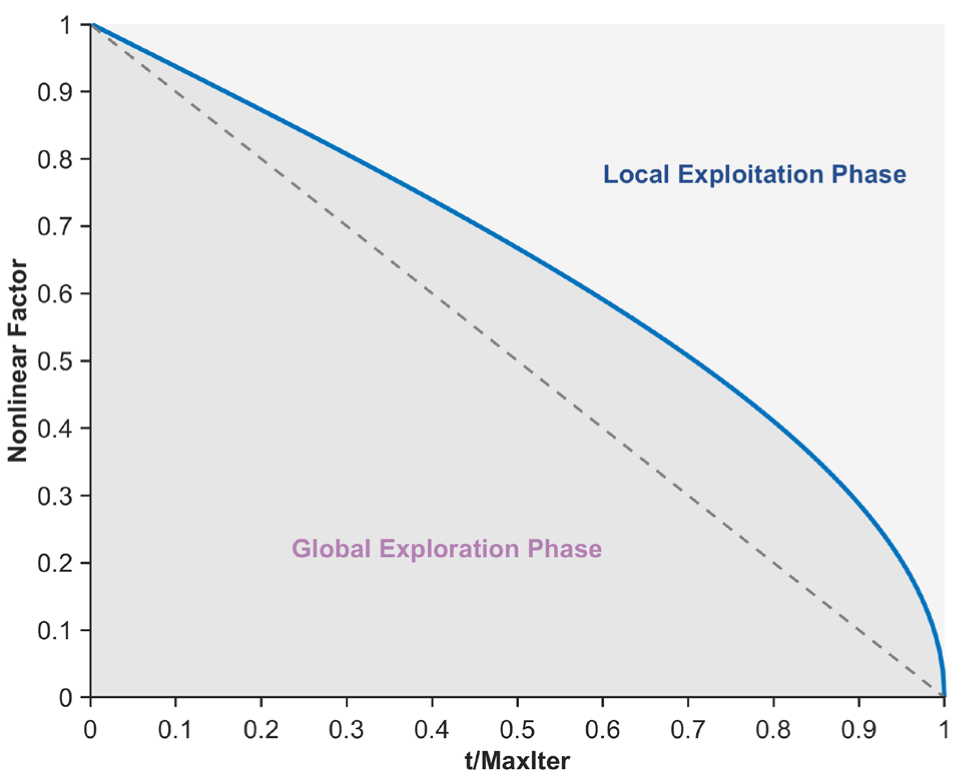
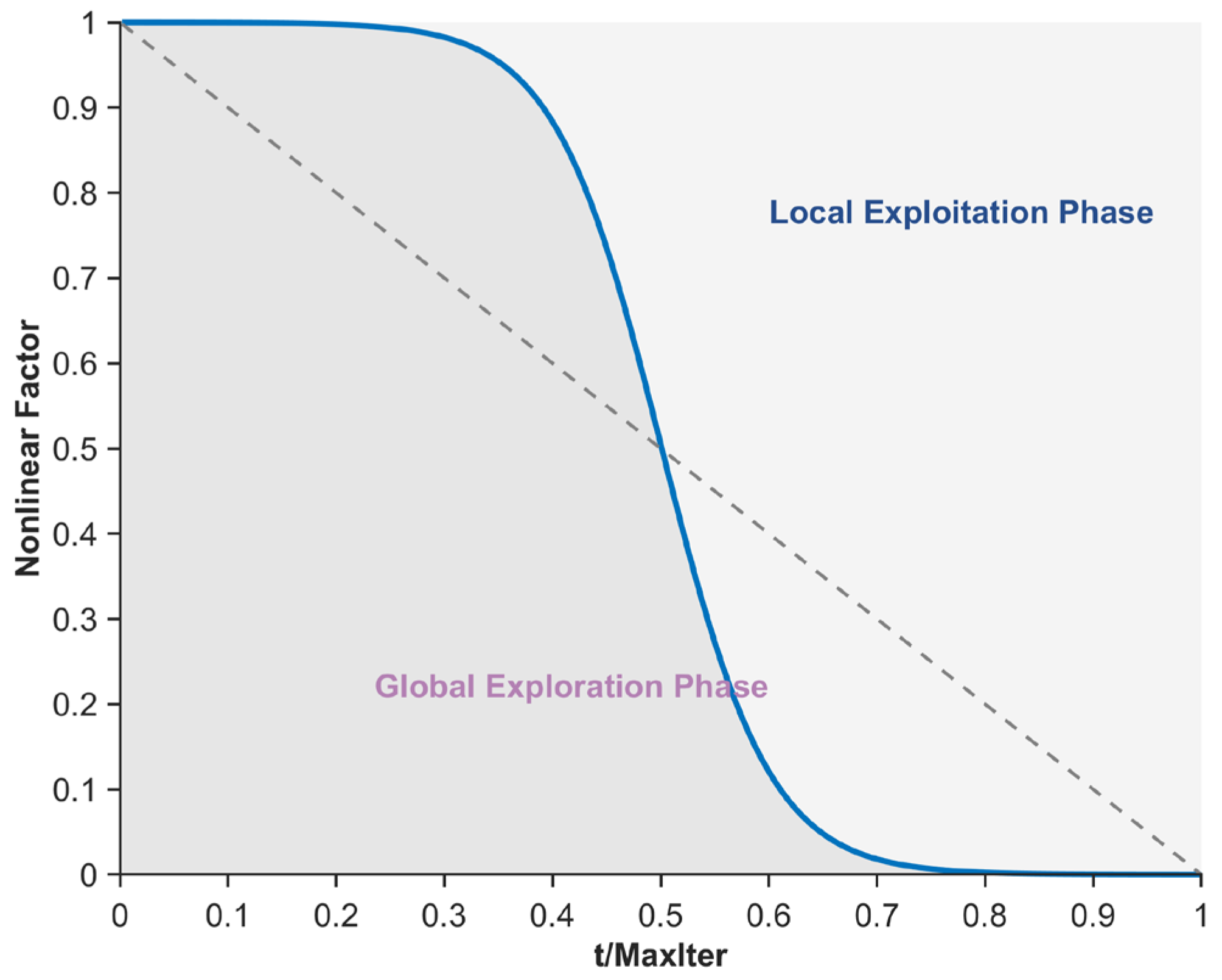
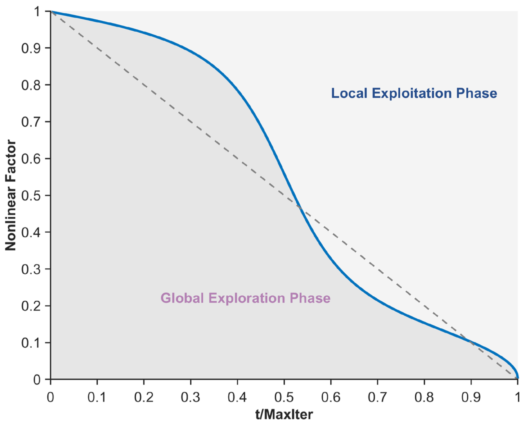
- The nonlinear factor is introduced to balance the algorithm’s exploration and exploitation phases, leveraging its adaptability and nonlinear curve characteristics.
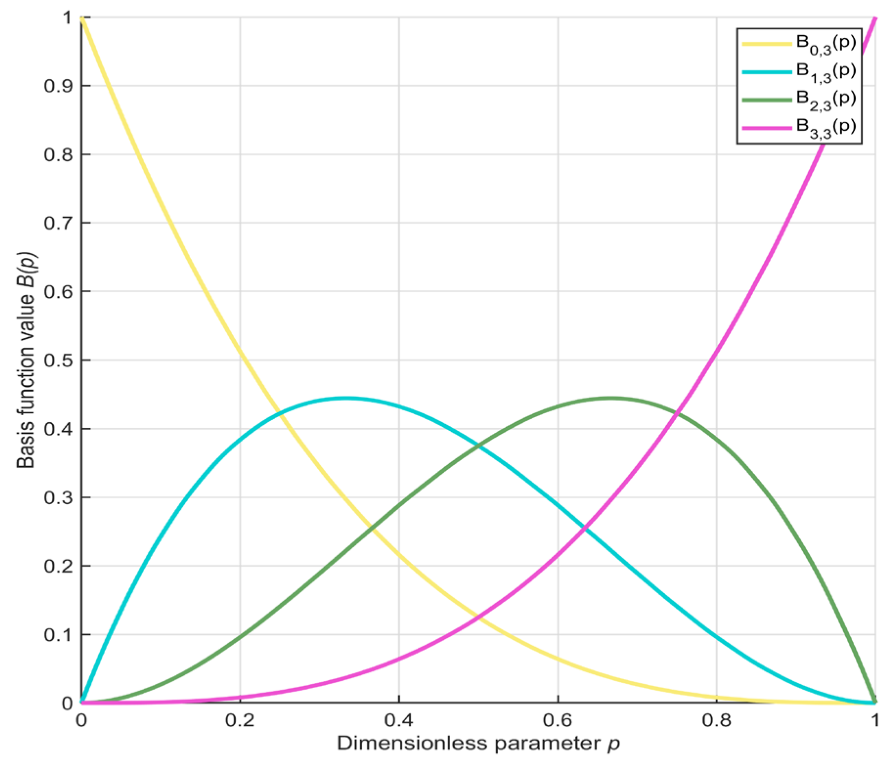
- The third-order Bernstein-guided strategy is proposed to strengthen the algorithm’s local exploitation capability by incorporating the weighted properties of third-order Bernstein polynomials, enabling comprehensive evaluation of individuals with diverse characteristics.
- By integrating these three learning strategies into the PO, an enhanced PO algorithm termed ANBPO is developed.
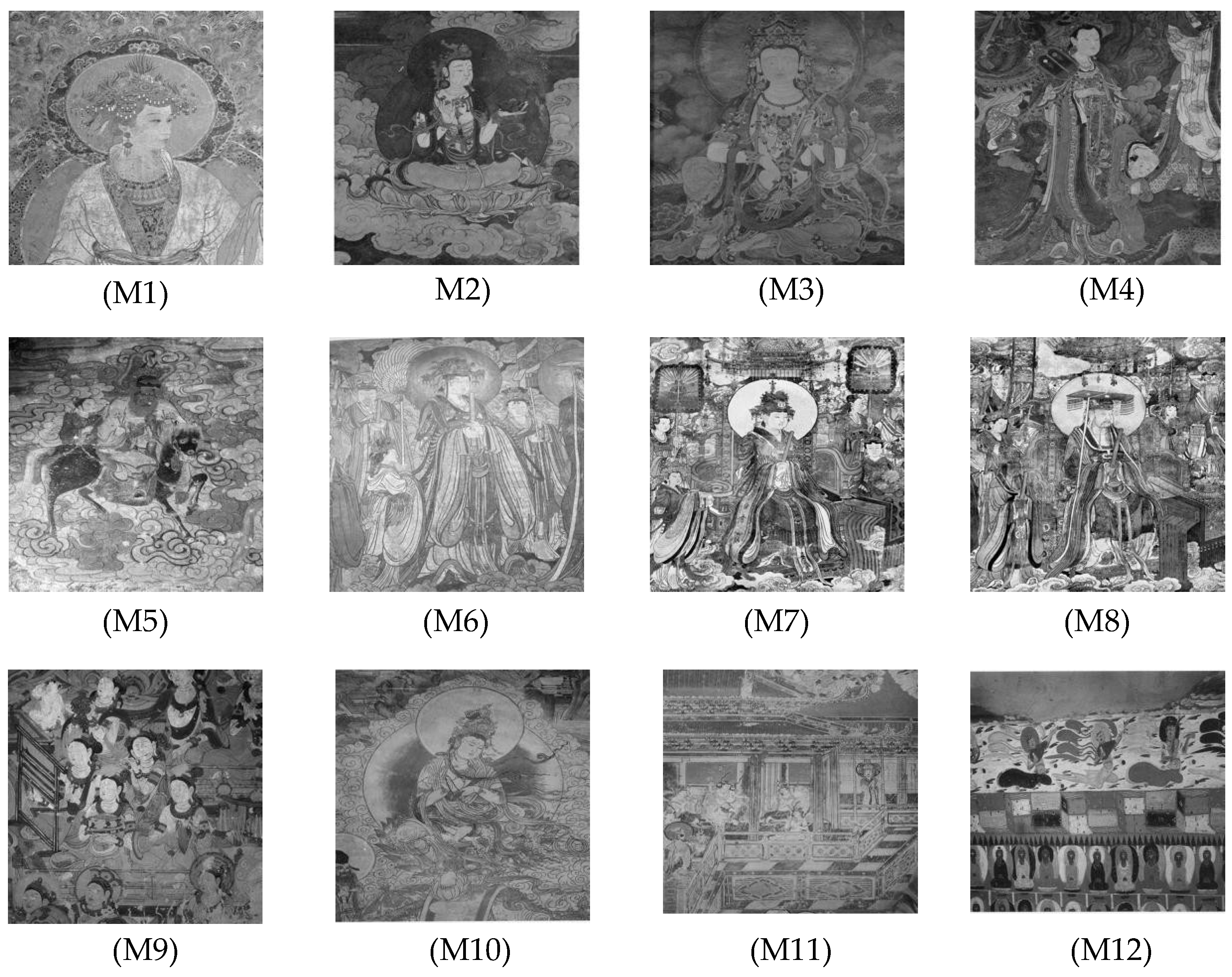
- Experimental segmentation of twelve mural images using ANBPO confirms its potential as a promising algorithm for mural image segmentation.
2. The Mathematical Model of the Parrot Optimizer
2.1. Population Initialization Phase
2.2. Foraging Behavior
2.3. Staying Behavior
2.4. Communicating Behavior
2.5. Fear of Strangers’ Behavior
2.6. Implementation of Parrot Optimizer
| Algorithm 1: Pseudo-code of PO |
|
3. The Mathematical Model of the ANBPO
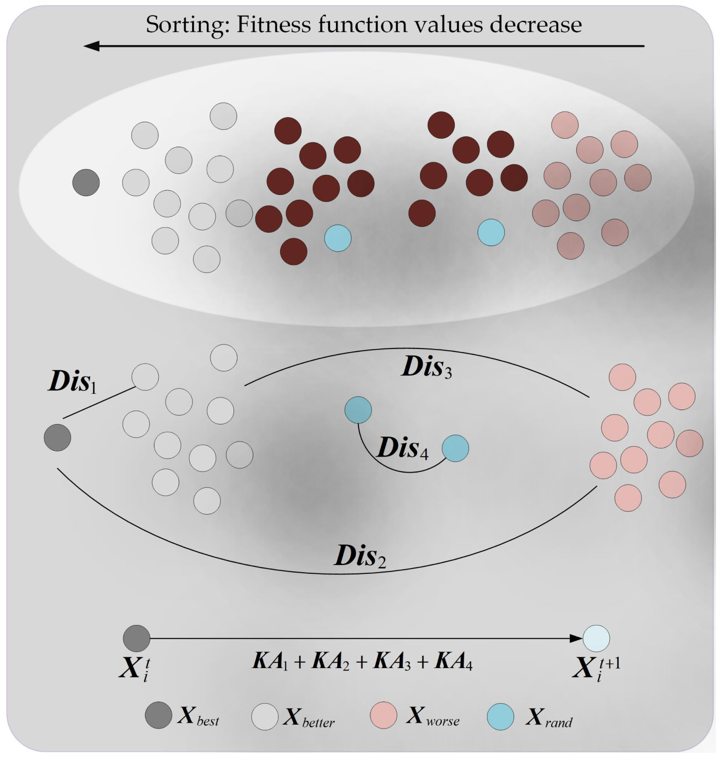
3.1. Adaptive Learning Strategy
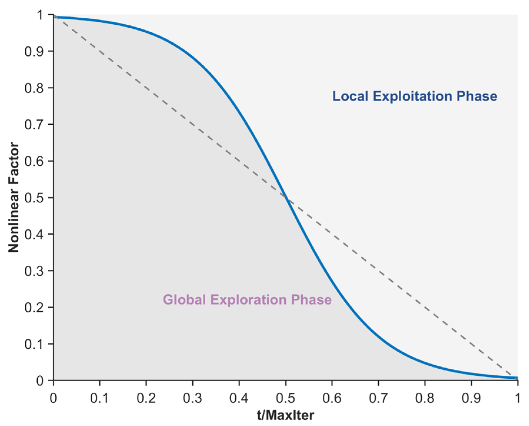
3.2. Nonlinear Factor
3.3. Third-Order Bernstein-Guided Strategy
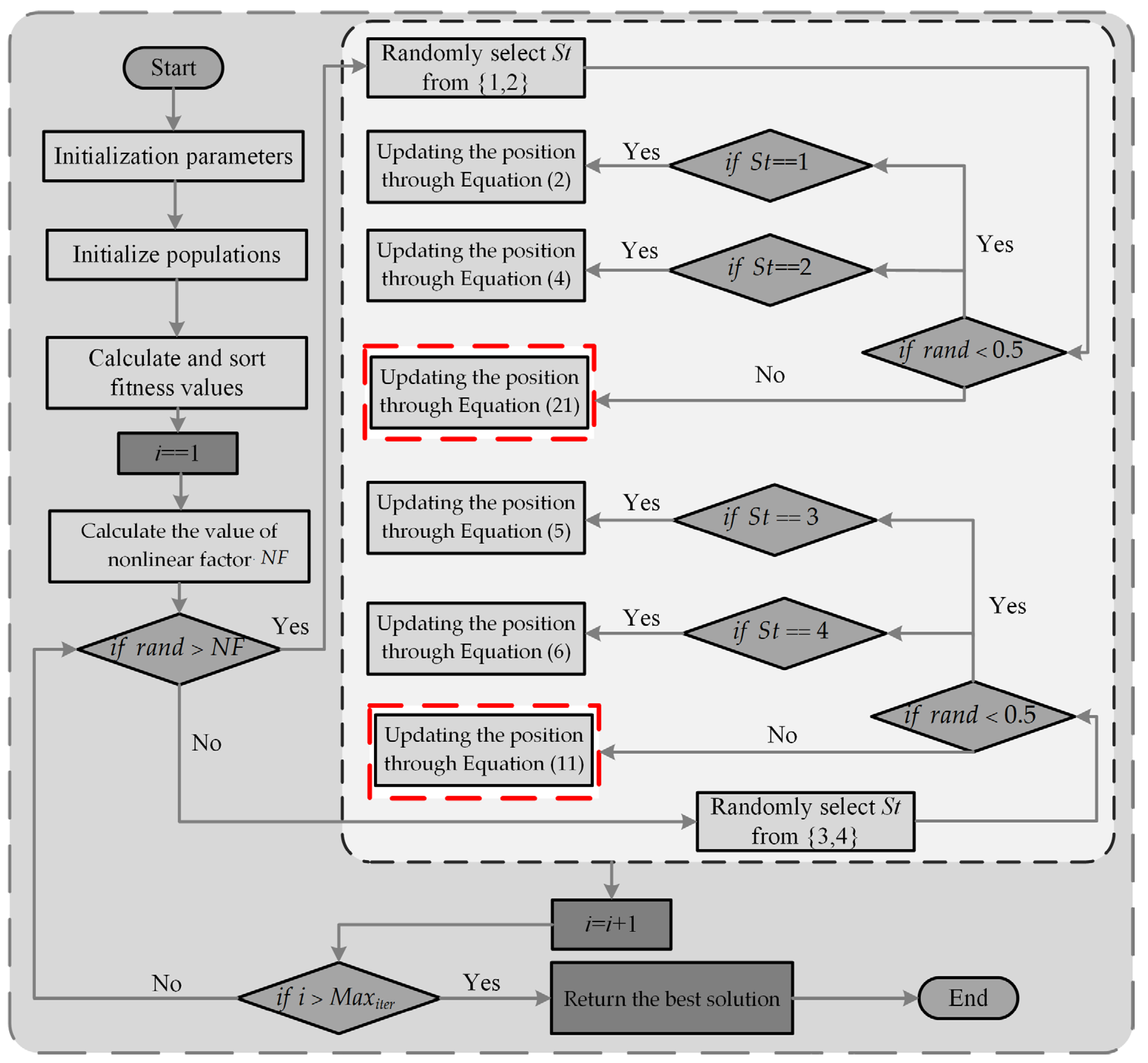
3.4. Implementation of ANBPO
| Algorithm 2: Pseudo-code of ANBPO |
|
4. Experimental Results on Mural Image Segmentation
4.1. The Concept of Otsu Segmentation Technique
4.2. Discussion of Experimental Results
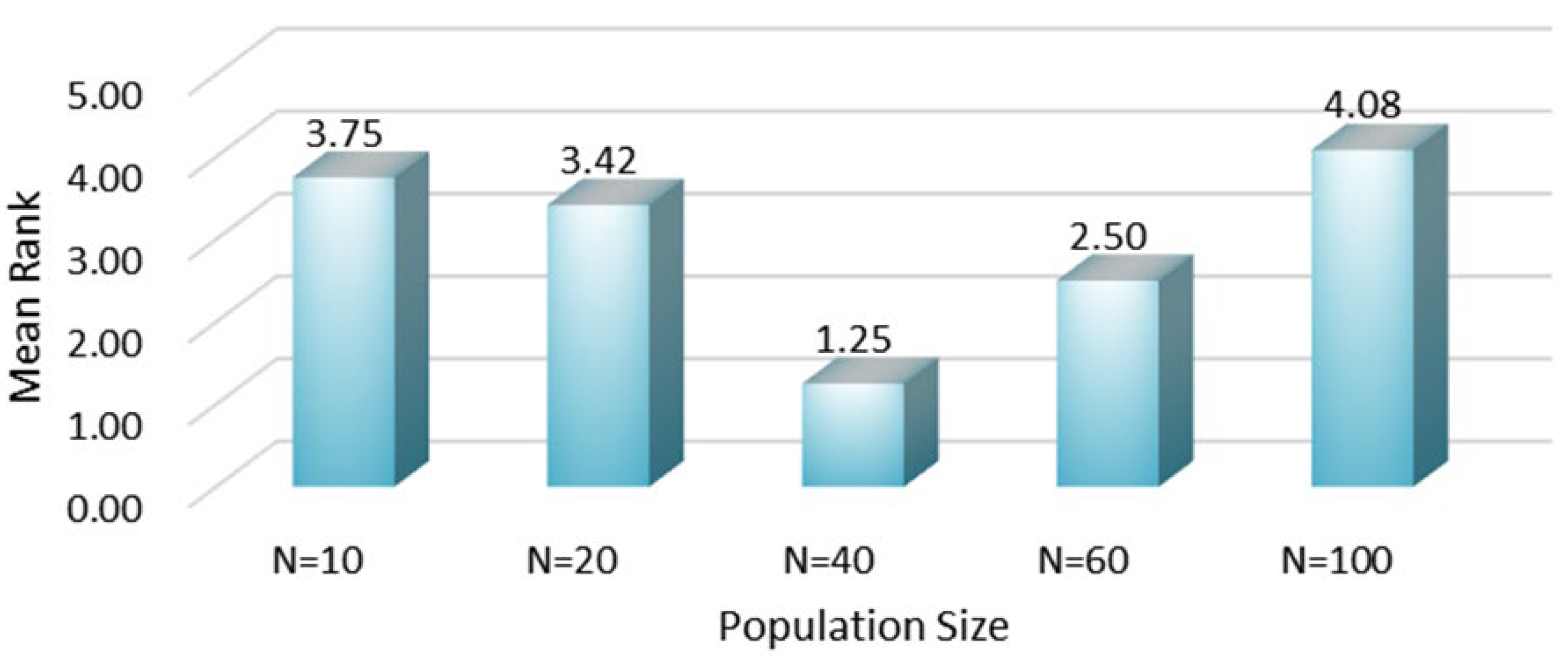
4.2.1. Parameter Sensitivity Analysis
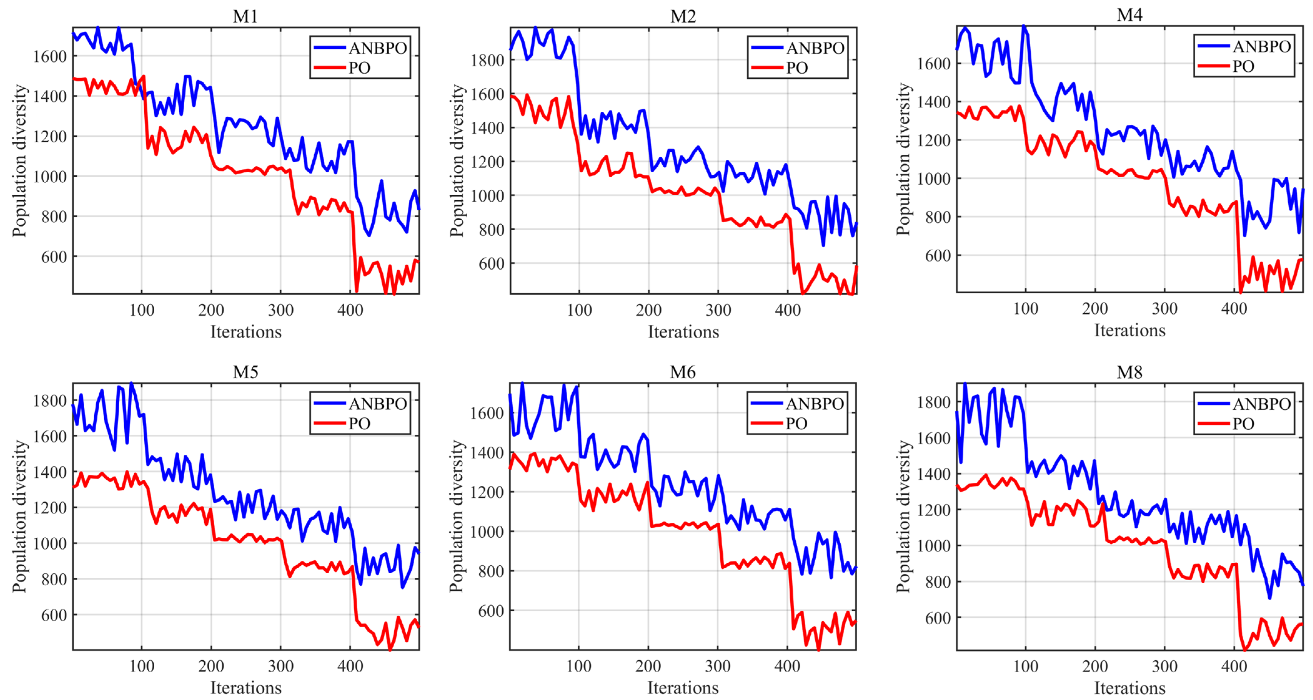
4.2.2. Population Diversity Analysis
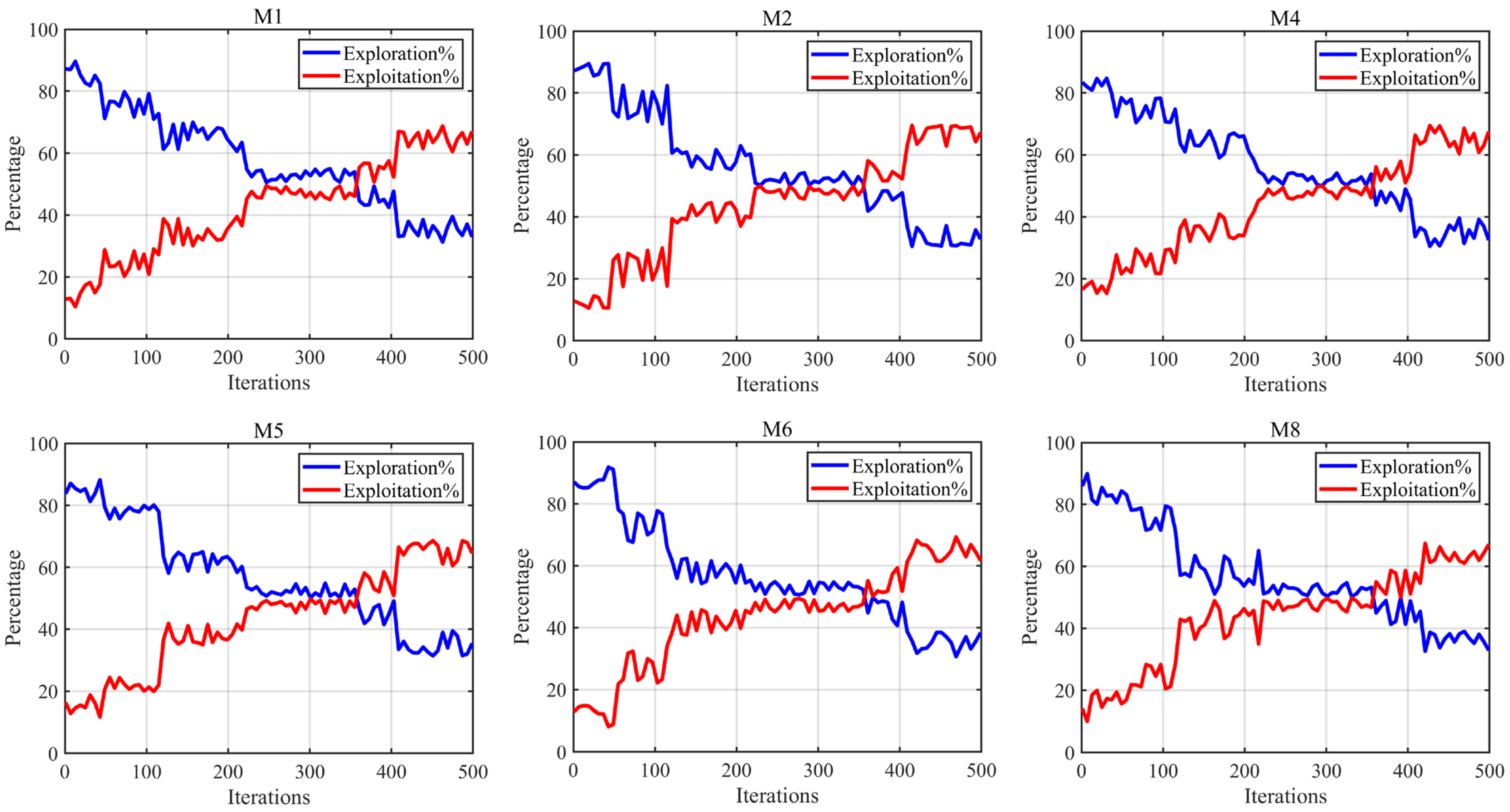
4.2.3. Exploration/Exploitation Ratio Analysis
4.2.4. Effectiveness of Strategies Analysis
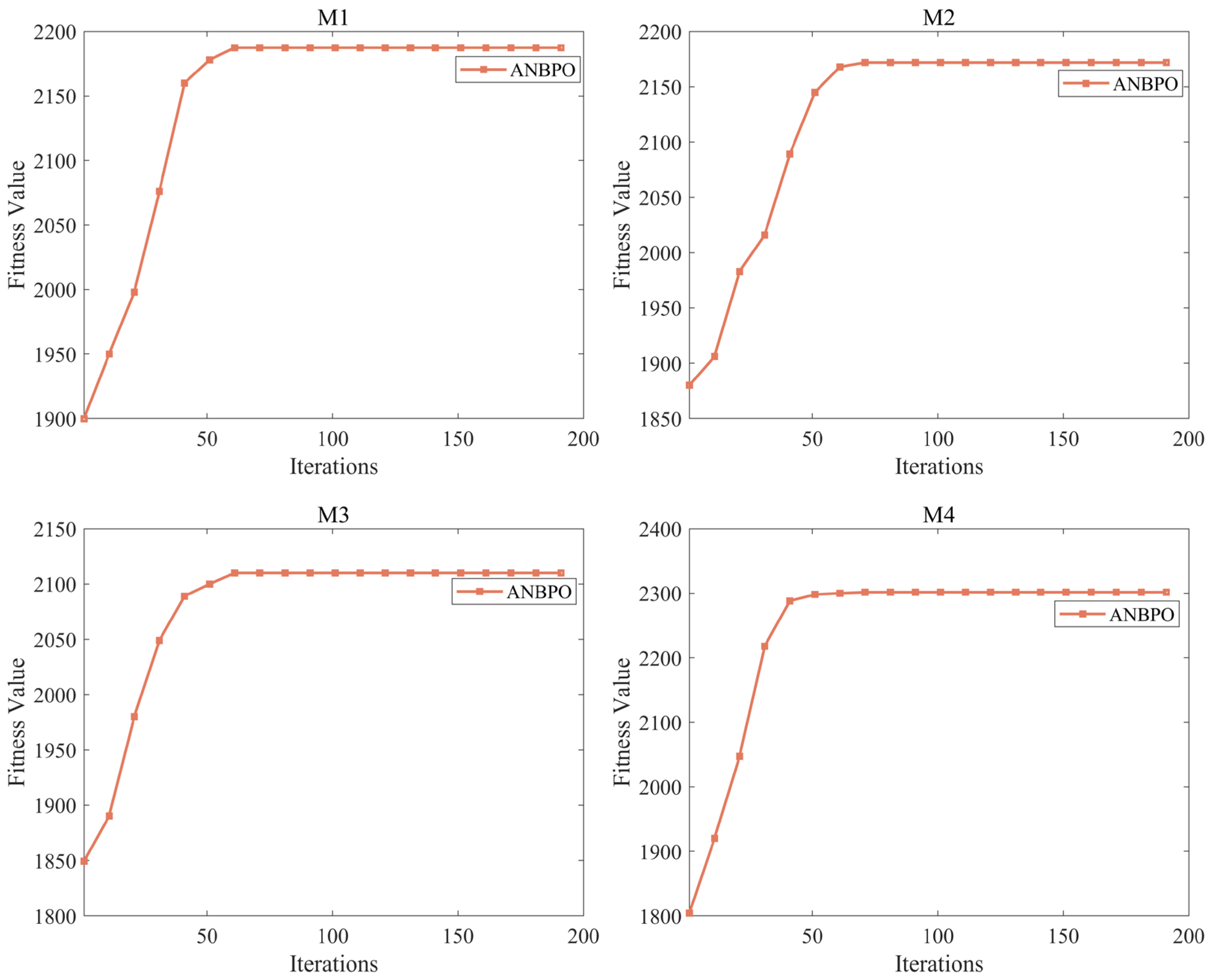
4.2.5. Fitness Function Values Analysis
4.2.6. Wilcoxon Rank Sum Test
4.2.7. Convergence Analysis
4.2.8. PSNR Analysis
4.2.9. SSIM Analysis
4.2.10. FSIM Analysis
4.2.11. Runtime Analysis
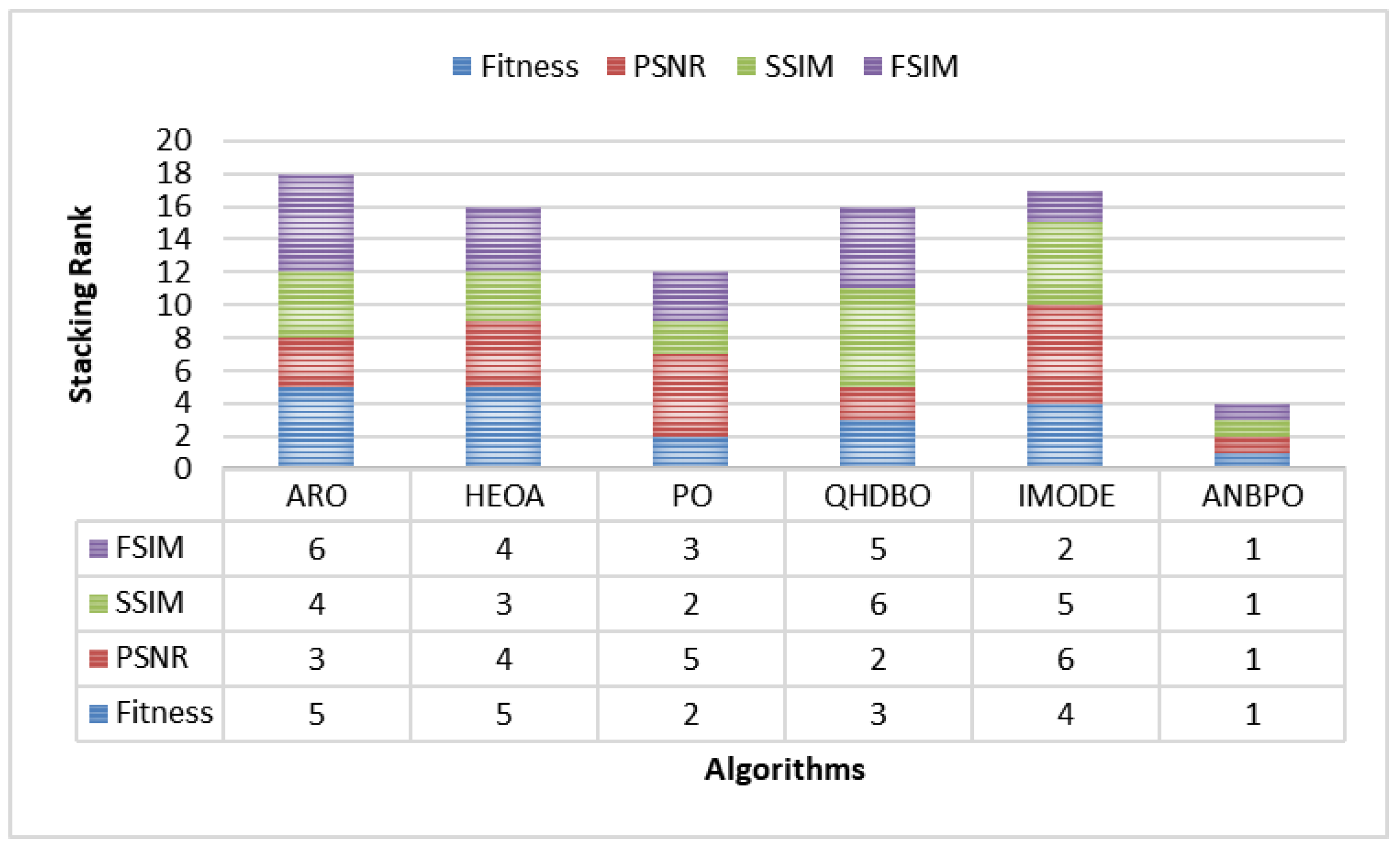
4.2.12. Comprehensive Analysis
5. Conclusions and Future Works
Author Contributions
Funding
Institutional Review Board Statement
Informed Consent Statement
Data Availability Statement
Acknowledgments
Conflicts of Interest
References
- Li, H. Intelligent restoration of ancient murals based on discrete differential algorithm. J. Comput. Methods Sci. Eng. 2021, 21, 803–814. [Google Scholar] [CrossRef]
- Jiao, L.J.; Wang, W.J.; Li, B.J.; Zhao, Q.S. Wutai Mountain mural inpainting based on improved block matching algorithm. J. Comput. Aid Des. Comput. Graph. 2019, 31, 119–125. [Google Scholar] [CrossRef]
- Yu, T.; Lin, C.; Zhang, S.; Ding, X.; Wu, J.; Zhang, J. End-to-end partial convolutions neural networks for Dunhuang grottoes wall-painting restoration. In Proceedings of the IEEE/CVF International Conference on Computer Vision Workshops, Seoul, Republic of Korea, 27–28 October 2019. [Google Scholar]
- Han, P.H.; Chen, Y.S.; Liu, I.S.; Jang, Y.P.; Tsai, L.; Chang, A.; Hung, Y.P. A compelling virtual tour of the dunhuang cave with an immersive head-mounted display. IEEE Comput. Graph. Appl. 2019, 40, 40–55. [Google Scholar] [CrossRef] [PubMed]
- Hou, M.; Cao, N.; Tan, L.; Lyu, S.; Zhou, P.; Xu, C. Extraction of hidden information under sootiness on murals based on hyperspectral image enhancement. Appl. Sci. 2019, 9, 3591. [Google Scholar] [CrossRef]
- Wu, M.; Li, M.; Zhang, Q. Feature Separation and Fusion to Optimise the Migration Model of Mural Painting Style in Tombs. Appl. Sci. 2024, 14, 2784. [Google Scholar] [CrossRef]
- Xiao, C.; Chen, Y.; Sun, C.; You, L.; Li, R. AM-ESRGAN: Super-resolution reconstruction of ancient murals based on attention mechanism and multi-level residual network. Electronics 2024, 13, 3142. [Google Scholar] [CrossRef]
- Zhou, Y.; Guo, M.; Ma, M. Mural image restoration with spatial geometric perception and progressive context refinement. Comput. Graph. 2025, 130, 104266. [Google Scholar] [CrossRef]
- Yu, Z.; Lyu, S.; Hou, M.; Sun, Y.; Li, L. A new method for extracting refined sketches of ancient murals. Sensors 2024, 24, 2213. [Google Scholar] [CrossRef]
- Abualigah, L.; Almotairi, K.H.; Elaziz, M.A. Multilevel thresholding image segmentation using meta-heuristic optimization algorithms: Comparative analysis, open challenges and new trends. Appl. Intell. 2023, 53, 11654–11704. [Google Scholar] [CrossRef]
- Khishe, M.; Mosavi, M.R. Chimp optimization algorithm. Expert Syst. Appl. 2020, 149, 113338. [Google Scholar] [CrossRef]
- Hashim, F.A.; Hussien, A.G. Snake Optimizer: A novel meta-heuristic optimization algorithm. Knowl.-Based Syst. 2022, 242, 108320. [Google Scholar] [CrossRef]
- Rocca, P.; Oliveri, G.; Massa, A. Differential evolution as applied to electromagnetics. IEEE Antennas Propag. Mag. 2011, 53, 38–49. [Google Scholar] [CrossRef]
- Holland, J.H. Genetic algorithms. Sci. Am. 1992, 267, 66–73. [Google Scholar] [CrossRef]
- Simon, D. Biogeography-based optimization. IEEE Trans. Evol. Comput. 2008, 12, 702–713. [Google Scholar] [CrossRef]
- Kennedy, J.; Eberhart, R. Particle swarm optimization. In Proceedings of the ICNN’95-International Conference on Neural Networks, Perth, WA, Australia, 27 November–1 December 1995; pp. 1942–1948. [Google Scholar]
- Li, S.; Chen, H.; Wang, M.; Heidari, A.A.; Mirjalili, S. Slime mould algorithm: A new method for stochastic optimization. Future Gener. Comput. Syst. 2020, 111, 300–323. [Google Scholar] [CrossRef]
- Mirjalili, S.; Lewis, A. The whale optimization algorithm. Adv. Eng. Softw. 2016, 95, 51–67. [Google Scholar] [CrossRef]
- Mirjalili, S.; Mirjalili, S.M.; Hatamlou, A. Multi-verse optimizer: A nature-inspired algorithm for global optimization. Neural Comput. Appl. 2016, 27, 495–513. [Google Scholar] [CrossRef]
- Zhao, W.; Wang, L.; Zhang, Z. Atom search optimization and its application to solve a hydrogeologic parameter estimation problem. Knowl.-Based Syst. 2019, 163, 283–304. [Google Scholar] [CrossRef]
- Kaveh, A.; Bakhshpoori, T. Water evaporation optimization: A novel physically inspired optimization algorithm. Comput. Struct. 2016, 167, 69–85. [Google Scholar] [CrossRef]
- Rao, R.V.; Savsani, V.J.; Vakharia, D.P. Teaching–learning-based optimization: A novel method for constrained mechanical design optimization problems. Comput.-Aided Des. 2011, 43, 303–315. [Google Scholar] [CrossRef]
- Moosavi, S.H.S.; Bardsiri, V.K. Poor and rich optimization algorithm: A new human-based and multi populations algorithm. Eng. Appl. Artif. Intell. 2019, 86, 165–181. [Google Scholar] [CrossRef]
- Shabani, A.; Asgarian, B.; Salido, M.; Gharebaghi, S.A. Search and rescue optimization algorithm: A new optimization method for solving constrained engineering optimization problems. Expert Syst. Appl. 2020, 161, 113698. [Google Scholar] [CrossRef]
- Houssein, E.H.; Abdalkarim, N.; Hussain, K.; Mohamed, E. Accurate multilevel thresholding image segmentation via oppositional Snake Optimization algorithm: Real cases with liver disease. Comput. Biol. Med. 2024, 169, 107922. [Google Scholar] [CrossRef] [PubMed]
- Wang, J.; Bao, Z.; Dong, H. An Improved Northern Goshawk Optimization Algorithm for Mural Image Segmentation. Biomimetics. 2025, 10, 373. [Google Scholar] [CrossRef] [PubMed]
- Qiao, L.; Liu, K.; Xue, Y.; Tang, W.; Salehnia, T. A multi-level thresholding image segmentation method using hybrid Arithmetic Optimization and Harris Hawks Optimizer algorithms. Expert Syst. Appl. 2024, 241, 122316. [Google Scholar] [CrossRef]
- Yuan, C.; Zhao, D.; Heidari, A.A.; Liu, L.; Chen, Y.; Wu, Z.; Chen, H. Artemisinin optimization based on malaria therapy: Algorithm and applications to medical image segmentation. Displays 2024, 84, 102740. [Google Scholar] [CrossRef]
- Chen, D.; Ge, Y.; Wan, Y.; Deng, Y.; Chen, Y.; Zou, F. Poplar optimization algorithm: A new meta-heuristic optimization technique for numerical optimization and image segmentation. Expert Syst. Appl. 2022, 200, 117118. [Google Scholar] [CrossRef]
- Wang, J.; Bei, J.; Song, H.; Zhang, H.; Zhang, P. A whale optimization algorithm with combined mutation and removing similarity for global optimization and multilevel thresholding image segmentation. Appl. Soft Comput. 2023, 137, 110130. [Google Scholar] [CrossRef]
- Das, A.; Namtirtha, A.; Dutta, A. Lévy–Cauchy arithmetic optimization algorithm combined with rough K-means for image segmentation. Appl. Soft Comput. 2023, 140, 110268. [Google Scholar] [CrossRef]
- Wang, Z.; Yu, F.; Wang, D.; Liu, T.; Hu, R. Multi-threshold segmentation of breast cancer images based on improved dandelion optimization algorithm. J. Supercomput. 2024, 80, 3849–3874. [Google Scholar] [CrossRef]
- Lian, J.; Hui, G.; Ma, L.; Zhu, T.; Wu, X.; Heidari, A.A.; Chen, H. Parrot optimizer: Algorithm and applications to medical problems. Comput. Biol. Med. 2024, 172, 108064. [Google Scholar] [CrossRef] [PubMed]
- Zhang, X.; Lin, Q. Three-learning strategy particle swarm algorithm for global optimization problems. Inf. Sci. 2022, 593, 289–313. [Google Scholar] [CrossRef]
- Wu, F.; Li, S.; Zhang, J.; Xie, R.; Yang, M. Bernstein-based oppositional-multiple learning and differential enhanced exponential distribution optimizer for real-world optimization problems. Eng. Appl. Artif. Intell. 2024, 138, 109370. [Google Scholar] [CrossRef]
- Huynh-Thu, Q.; Ghanbari, M. Scope of validity of PSNR in image/video quality assessment. Electron. Lett. 2008, 44, 800–801. [Google Scholar] [CrossRef]
- Wang, Z.; Bovik, A.C.; Sheikh, H.R.; Simoncelli, E.P. Image quality assessment: From error visibility to structural similarity. IEEE Trans. Image Process. 2004, 13, 600–612. [Google Scholar] [CrossRef]
- Zhang, L.; Zhang, L.; Mou, X.; Zhang, D. FSIM: A feature similarity index for image quality assessment. IEEE Trans. Image Process. 2011, 20, 2378–2386. [Google Scholar] [CrossRef]
- Taheri, A.; RahimiZadeh, K.; Beheshti, A.; Baumbach, J.; Rao, R.V.; Mirjalili, S.; Gandomi, A.H. Partial reinforcement optimizer: An evolutionary optimization algorithm. Expert Syst. Appl. 2024, 238, 122070. [Google Scholar] [CrossRef]
- Lian, J.; Hui, G. Human evolutionary optimization algorithm. Expert Syst. Appl. 2024, 241, 122638. [Google Scholar] [CrossRef]
- Zhu, F.; Li, G.; Tang, H.; Li, Y.; Lv, X.; Wang, X. Dung beetle optimization algorithm based on quantum computing and multi-strategy fusion for solving engineering problems. Expert Syst. Appl. 2024, 236, 121219. [Google Scholar] [CrossRef]
- Sallam, K.M.; Elsayed, S.M.; Chakrabortty, R.K.; Ryan, M.J. Improved multi-operator differential evolution algorithm for solving unconstrained problems. In Proceedings of the 2020 IEEE Congress on Evolutionary Computation (CEC), Glasgow, UK, 19–24 July 2020; pp. 1–8. [Google Scholar]


| Algorithms | Year | Parameter Settings |
|---|---|---|
| PRO [39] | 2024 | |
| HEOA [40] | 2024 | |
| PO [33] | 2024 | No Parameters |
| QHDBO [41] | 2024 | |
| IMODE [42] | 2020 |
| Fun | nTH = 2 | nTH = 4 | nTH = 6 | nTH = 8 |
|---|---|---|---|---|
| M1 | 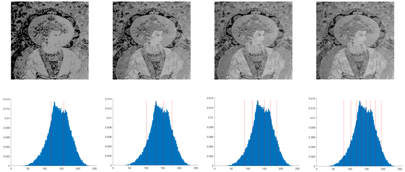 | |||
| M2 | 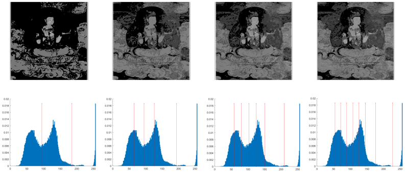 | |||
| M3 | 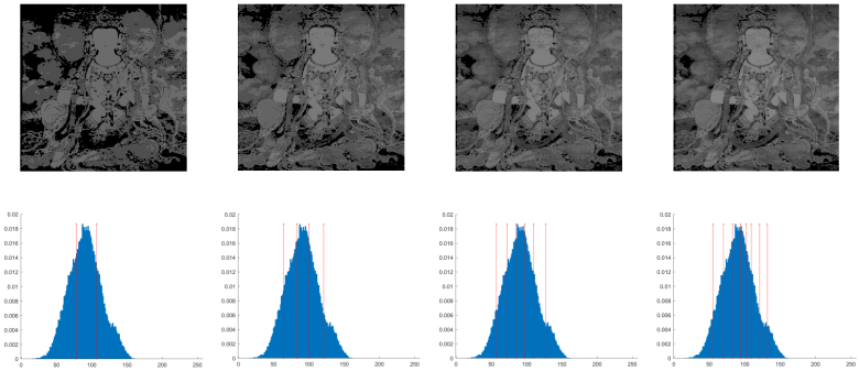 | |||
| M4 |  | |||
| M5 |  | |||
| M6 | 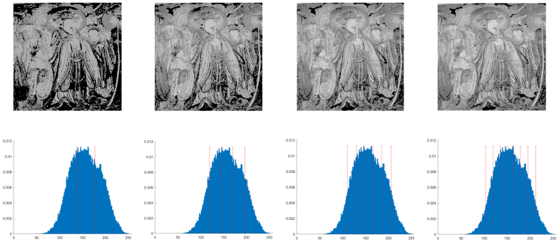 | |||
| M7 | 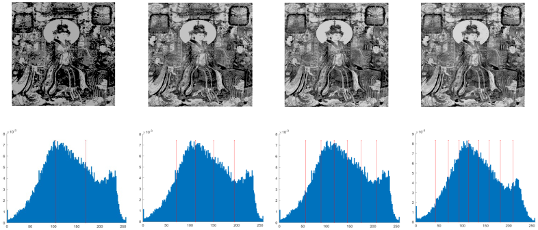 | |||
| M8 | 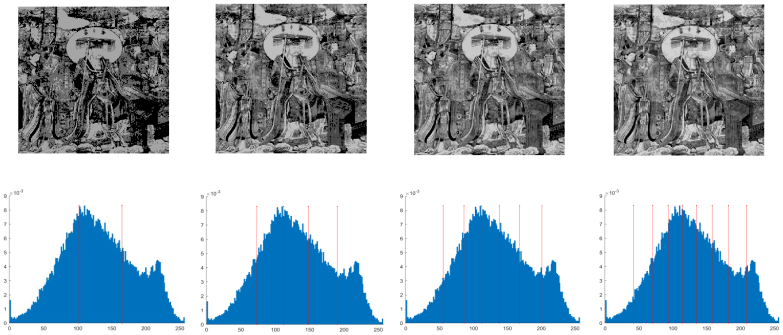 | |||
| M9 |  | |||
| M10 | 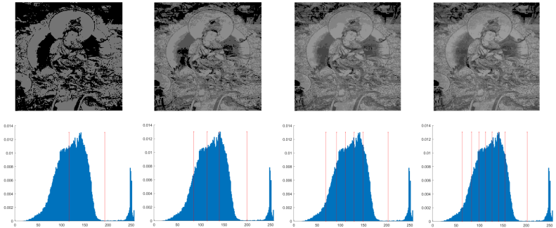 | |||
| M11 |  | |||
| M12 |  | |||
| Fun | nTH | PRO | HEOA | PO | QHDBO | IMODE | ANBPO | ||||||
| Mean | Std | Mean | Std | Mean | Std | Mean | Std | Mean | Std | Mean | Std | ||
| M1 | 2 | 1.813 × 10+03 | 8.352 × 10−01 | 1.729 × 10+03 | 3.675 × 10−01 | 1.850 × 10+03 | 2.879 × 10−01 | 1.806 × 10+03 | 3.554 × 10−01 | 1.878 × 10+03 | 3.003 × 10−01 | 1.968 × 10+03 | 3.856 × 10−03 |
| 4 | 1.960 × 10+03 | 3.968 × 10−01 | 1.974 × 10+03 | 4.176 × 10−01 | 1.977 × 10+03 | 5.018 × 10−01 | 1.914 × 10+03 | 2.319 × 10−03 | 1.957 × 10+03 | 9.386 × 10−02 | 2.055 × 10+03 | 6.688 × 10−03 | |
| 6 | 2.100 × 10+03 | 9.918 × 10−01 | 2.002 × 10+03 | 4.686 × 10−01 | 2.087 × 10+03 | 9.665 × 10−01 | 2.089 × 10+03 | 7.851 × 10−01 | 2.079 × 10+03 | 6.825 × 10−01 | 2.187 × 10+03 | 2.458 × 10−03 | |
| 8 | 2.137 × 10+03 | 1.707 × 10−01 | 2.125 × 10+03 | 6.466 × 10−01 | 2.171 × 10+03 | 3.681 × 10−01 | 2.175 × 10+03 | 6.164 × 10−02 | 2.177 × 10+03 | 9.645 × 10−01 | 2.281 × 10+03 | 4.850 × 10−03 | |
| M2 | 2 | 1.862 × 10+03 | 5.941 × 10−01 | 1.878 × 10+03 | 7.653 × 10−01 | 1.802 × 10+03 | 2.357 × 10−01 | 1.887 × 10+03 | 2.251 × 10−01 | 1.871 × 10+03 | 5.155 × 10−01 | 1.901 × 10+03 | 9.242 × 10−03 |
| 4 | 1.998 × 10+03 | 1.871 × 10−01 | 1.958 × 10+03 | 5.132 × 10−02 | 1.994 × 10+03 | 7.300 × 10−01 | 1.927 × 10+03 | 1.509 × 10−01 | 1.959 × 10+03 | 8.456 × 10−01 | 2.036 × 10+03 | 8.011 × 10−03 | |
| 6 | 2.051 × 10+03 | 5.163 × 10−01 | 2.090 × 10+03 | 5.548 × 10−02 | 2.051 × 10+03 | 4.892 × 10−01 | 2.027 × 10+03 | 1.213 × 10−01 | 2.069 × 10+03 | 2.477 × 10−01 | 2.172 × 10+03 | 3.464 × 10−03 | |
| 8 | 2.161 × 10+03 | 5.903 × 10−01 | 2.188 × 10+03 | 3.963 × 10−02 | 2.177 × 10+03 | 2.244 × 10−01 | 2.187 × 10+03 | 7.401 × 10−01 | 2.161 × 10+03 | 1.428 × 10−01 | 2.281 × 10+03 | 1.847 × 10−03 | |
| M3 | 2 | 1.704 × 10+03 | 5.725 × 10−01 | 1.702 × 10+03 | 5.769 × 10−01 | 1.757 × 10+03 | 4.049 × 10−01 | 1.763 × 10+03 | 7.642 × 10−01 | 1.722 × 10+03 | 3.311 × 10−01 | 1.952 × 10+03 | 2.416 × 10−03 |
| 4 | 1.910 × 10+03 | 4.311 × 10−01 | 1.961 × 10+03 | 5.306 × 10−01 | 1.943 × 10+03 | 2.542 × 10−02 | 1.945 × 10+03 | 3.695 × 10−01 | 1.967 × 10+03 | 2.824 × 10−01 | 2.069 × 10+03 | 2.703 × 10−01 | |
| 6 | 2.051 × 10+03 | 6.846 × 10−01 | 2.035 × 10+03 | 5.228 × 10−01 | 2.027 × 10+03 | 3.230 × 10−01 | 2.093 × 10+03 | 5.396 × 10−01 | 2.042 × 10+03 | 1.183 × 10−01 | 2.110 × 10+03 | 9.911 × 10−01 | |
| 8 | 2.107 × 10+03 | 7.664 × 10−01 | 2.111 × 10+03 | 5.327 × 10−01 | 2.107 × 10+03 | 5.773 × 10−01 | 2.160 × 10+03 | 5.689 × 10−01 | 2.104 × 10+03 | 7.490 × 10−01 | 2.230 × 10+03 | 9.125 × 10−01 | |
| M4 | 2 | 1.915 × 10+03 | 1.423 × 10−01 | 2.072 × 10+03 | 2.723 × 10−01 | 2.067 × 10+03 | 2.441 × 10−01 | 2.061 × 10+03 | 7.754 × 10−02 | 1.924 × 10+03 | 4.893 × 10−01 | 2.118 × 10+03 | 4.486 × 10−03 |
| 4 | 2.109 × 10+03 | 5.008 × 10−01 | 2.198 × 10+03 | 6.679 × 10−01 | 2.138 × 10+03 | 2.440 × 10−01 | 2.106 × 10+03 | 1.184 × 10−01 | 2.161 × 10+03 | 6.653 × 10−01 | 2.212 × 10+03 | 3.122 × 10−03 | |
| 6 | 2.254 × 10+03 | 2.135 × 10−01 | 2.220 × 10+03 | 3.077 × 10−01 | 2.296 × 10+03 | 4.107 × 10−01 | 2.220 × 10+03 | 1.161 × 10−01 | 2.265 × 10+03 | 2.023 × 10−02 | 2.302 × 10+03 | 5.954 × 10−03 | |
| 8 | 2.340 × 10+03 | 6.163 × 10−01 | 2.359 × 10+03 | 6.875 × 10−01 | 2.316 × 10+03 | 7.406 × 10−01 | 2.357 × 10+03 | 3.099 × 10−01 | 2.326 × 10+03 | 9.467 × 10−01 | 2.488 × 10+03 | 7.470 × 10−03 | |
| M5 | 2 | 1.965 × 10+03 | 4.318 × 10−01 | 1.914 × 10+03 | 9.641 × 10−01 | 2.068 × 10+03 | 6.459 × 10−01 | 1.951 × 10+03 | 2.746 × 10−02 | 2.069 × 10+03 | 8.577 × 10−01 | 2.184 × 10+03 | 3.591 × 10−03 |
| 4 | 2.183 × 10+03 | 9.105 × 10−01 | 2.168 × 10+03 | 4.511 × 10−01 | 2.122 × 10+03 | 9.968 × 10−01 | 2.154 × 10+03 | 1.662 × 10−01 | 2.141 × 10+03 | 6.976 × 10−01 | 2.140 × 10+03 | 3.207 × 10−03 | |
| 6 | 2.210 × 10+03 | 8.396 × 10−01 | 2.214 × 10+03 | 1.822 × 10−01 | 2.279 × 10+03 | 2.783 × 10−02 | 2.294 × 10+03 | 5.123 × 10−01 | 2.294 × 10+03 | 3.414 × 10−01 | 2.335 × 10+03 | 7.437 × 10−03 | |
| 8 | 2.380 × 10+03 | 3.985 × 10−01 | 2.379 × 10+03 | 4.268 × 10−02 | 2.397 × 10+03 | 8.447 × 10−01 | 2.385 × 10+03 | 8.494 × 10−02 | 2.355 × 10+03 | 8.251 × 10−02 | 2.446 × 10+03 | 5.010 × 10−03 | |
| M6 | 2 | 2.146 × 10+03 | 9.882 × 10−01 | 2.233 × 10+03 | 4.068 × 10−01 | 2.140 × 10+03 | 8.554 × 10−01 | 2.172 × 10+03 | 5.330 × 10−01 | 2.215 × 10+03 | 4.111 × 10−01 | 2.382 × 10+03 | 8.480 × 10−03 |
| 4 | 2.321 × 10+03 | 3.821 × 10−01 | 2.327 × 10+03 | 1.676 × 10−01 | 2.385 × 10+03 | 7.740 × 10−01 | 2.363 × 10+03 | 5.560 × 10−01 | 2.390 × 10+03 | 9.804 × 10−01 | 2.484 × 10+03 | 9.184 × 10−03 | |
| 6 | 2.418 × 10+03 | 9.068 × 10−01 | 2.438 × 10+03 | 6.645 × 10−01 | 2.462 × 10+03 | 7.520 × 10−01 | 2.486 × 10+03 | 9.283 × 10−01 | 2.489 × 10+03 | 4.272 × 10−01 | 2.582 × 10+03 | 6.756 × 10−03 | |
| 8 | 2.502 × 10+03 | 2.733 × 10−01 | 2.541 × 10+03 | 7.706 × 10−01 | 2.527 × 10+03 | 4.829 × 10−01 | 2.527 × 10+03 | 1.037 × 10−01 | 2.543 × 10+03 | 5.780 × 10−01 | 2.582 × 10+03 | 1.078 × 10−03 | |
| M7 | 2 | 1.830 × 10+03 | 9.584 × 10−01 | 1.878 × 10+03 | 9.725 × 10−02 | 1.884 × 10+03 | 4.415 × 10−03 | 1.867 × 10+03 | 9.208 × 10−01 | 1.823 × 10+03 | 2.722 × 10−01 | 1.991 × 10+03 | 4.926 × 10−03 |
| 4 | 1.937 × 10+03 | 8.134 × 10−01 | 1.919 × 10+03 | 5.443 × 10−01 | 1.996 × 10+03 | 8.147 × 10−01 | 1.935 × 10+03 | 1.655 × 10−01 | 1.926 × 10+03 | 9.502 × 10−01 | 2.092 × 10+03 | 2.248 × 10−03 | |
| 6 | 2.086 × 10+03 | 7.735 × 10−01 | 2.031 × 10+03 | 3.954 × 10−01 | 2.031 × 10+03 | 1.736 × 10−01 | 2.064 × 10+03 | 5.458 × 10−01 | 2.012 × 10+03 | 6.190 × 10−01 | 2.125 × 10+03 | 9.585 × 10−03 | |
| 8 | 2.122 × 10+03 | 3.275 × 10−01 | 2.119 × 10+03 | 2.701 × 10−01 | 2.129 × 10+03 | 1.146 × 10−01 | 2.151 × 10+03 | 6.068 × 10−01 | 2.136 × 10+03 | 7.348 × 10−01 | 2.150 × 10+03 | 3.670 × 10−01 | |
| M8 | 2 | 2.193 × 10+03 | 8.043 × 10−01 | 2.168 × 10+03 | 2.752 × 10−01 | 2.174 × 10+03 | 9.430 × 10−01 | 2.246 × 10+03 | 9.186 × 10−01 | 2.256 × 10+03 | 1.558 × 10−01 | 2.381 × 10+03 | 6.996 × 10−01 |
| 4 | 2.346 × 10+03 | 6.934 × 10−01 | 2.308 × 10+03 | 7.018 × 10−01 | 2.397 × 10+03 | 9.771 × 10−02 | 2.384 × 10+03 | 8.133 × 10−01 | 2.306 × 10+03 | 6.269 × 10−01 | 2.460 × 10+03 | 3.807 × 10−03 | |
| 6 | 2.429 × 10+03 | 2.730 × 10−01 | 2.411 × 10+03 | 6.778 × 10−01 | 2.403 × 10+03 | 4.274 × 10−01 | 2.439 × 10+03 | 7.378 × 10−01 | 2.466 × 10+03 | 2.616 × 10−01 | 2.577 × 10+03 | 2.923 × 10−03 | |
| 8 | 2.516 × 10+03 | 4.396 × 10−01 | 2.522 × 10+03 | 8.564 × 10−01 | 2.527 × 10+03 | 6.899 × 10−01 | 2.543 × 10+03 | 3.740 × 10−01 | 2.548 × 10+03 | 8.250 × 10−01 | 2.578 × 10+03 | 2.502 × 10−04 | |
| M9 | 2 | 1.899 × 10+03 | 6.740 × 10−01 | 1.720 × 10+03 | 4.882 × 10−01 | 1.803 × 10+03 | 5.393 × 10−01 | 1.751 × 10+03 | 5.164 × 10−01 | 1.703 × 10+03 | 2.144 × 10−01 | 1.990 × 10+03 | 1.143 × 10−03 |
| 4 | 1.936 × 10+03 | 2.621 × 10−01 | 1.918 × 10+03 | 8.270 × 10−01 | 1.938 × 10+03 | 2.595 × 10−01 | 1.928 × 10+03 | 3.427 × 10−01 | 1.992 × 10+03 | 7.983 × 10−01 | 2.072 × 10+03 | 9.555 × 10−03 | |
| 6 | 2.080 × 10+03 | 4.779 × 10−01 | 2.091 × 10+03 | 5.835 × 10−01 | 2.091 × 10+03 | 3.184 × 10−01 | 2.076 × 10+03 | 2.208 × 10−01 | 2.044 × 10+03 | 6.504 × 10−01 | 2.116 × 10+03 | 7.134 × 10−03 | |
| 8 | 2.188 × 10+03 | 3.904 × 10−01 | 2.110 × 10+03 | 1.766 × 10−01 | 2.148 × 10+03 | 6.578 × 10−01 | 2.117 × 10+03 | 3.469 × 10−01 | 2.109 × 10+03 | 8.407 × 10−01 | 2.293 × 10+03 | 7.798 × 10−03 | |
| M10 | 2 | 1.719 × 10+03 | 1.438 × 10−02 | 1.743 × 10+03 | 7.830 × 10−01 | 1.884 × 10+03 | 6.177 × 10−01 | 1.895 × 10+03 | 6.832 × 10−01 | 1.870 × 10+03 | 7.778 × 10−02 | 1.969 × 10+03 | 6.079 × 10−03 |
| 4 | 1.909 × 10+03 | 3.621 × 10−01 | 1.910 × 10+03 | 4.601 × 10−01 | 1.912 × 10+03 | 4.820 × 10−01 | 1.956 × 10+03 | 4.957 × 10−01 | 1.916 × 10+03 | 2.702 × 10−01 | 2.051 × 10+03 | 6.521 × 10−03 | |
| 6 | 2.081 × 10+03 | 1.636 × 10−01 | 2.054 × 10+03 | 8.964 × 10−01 | 2.037 × 10+03 | 1.358 × 10−01 | 2.008 × 10+03 | 5.350 × 10−01 | 2.066 × 10+03 | 2.550 × 10−01 | 2.154 × 10+03 | 3.527 × 10−03 | |
| 8 | 2.125 × 10+03 | 4.139 × 10−01 | 2.121 × 10+03 | 4.987 × 10−01 | 2.170 × 10+03 | 2.339 × 10−01 | 2.162 × 10+03 | 3.894 × 10−02 | 2.132 × 10+03 | 4.937 × 10−01 | 2.249 × 10+03 | 1.102 × 10−03 | |
| M11 | 2 | 1.787 × 10+03 | 5.036 × 10−01 | 1.848 × 10+03 | 2.007 × 10−01 | 1.750 × 10+03 | 8.128 × 10−03 | 1.817 × 10+03 | 1.156 × 10−01 | 1.845 × 10+03 | 7.805 × 10−01 | 1.973 × 10+03 | 3.508 × 10−03 |
| 4 | 1.988 × 10+03 | 7.509 × 10−01 | 1.998 × 10+03 | 8.576 × 10−02 | 1.963 × 10+03 | 4.031 × 10−01 | 1.928 × 10+03 | 2.261 × 10−01 | 1.932 × 10+03 | 6.414 × 10−01 | 2.048 × 10+03 | 4.671 × 10−01 | |
| 6 | 2.077 × 10+03 | 7.419 × 10−02 | 2.068 × 10+03 | 1.906 × 10−01 | 2.064 × 10+03 | 3.102 × 10−01 | 2.025 × 10+03 | 2.401 × 10−02 | 2.036 × 10+03 | 2.432 × 10−01 | 2.182 × 10+03 | 9.253 × 10−01 | |
| 8 | 2.165 × 10+03 | 8.111 × 10−01 | 2.150 × 10+03 | 1.194 × 10−01 | 2.168 × 10+03 | 1.836 × 10−01 | 2.116 × 10+03 | 3.910 × 10−01 | 2.156 × 10+03 | 1.398 × 10−01 | 2.228 × 10+03 | 8.540 × 10−01 | |
| M12 | 2 | 1.923 × 10+03 | 6.196 × 10−01 | 2.098 × 10+03 | 4.279 × 10−01 | 1.925 × 10+03 | 7.119 × 10−01 | 2.085 × 10+03 | 3.927 × 10−01 | 2.060 × 10+03 | 7.114 × 10−02 | 2.169 × 10+03 | 3.564 × 10−03 |
| 4 | 2.152 × 10+03 | 5.787 × 10−01 | 2.142 × 10+03 | 9.525 × 10−01 | 2.164 × 10+03 | 3.607 × 10−01 | 2.131 × 10+03 | 3.459 × 10−01 | 2.132 × 10+03 | 5.931 × 10−01 | 2.277 × 10+03 | 3.058 × 10−03 | |
| 6 | 2.284 × 10+03 | 2.190 × 10−02 | 2.233 × 10+03 | 6.926 × 10−01 | 2.275 × 10+03 | 3.104 × 10−01 | 2.295 × 10+03 | 9.227 × 10−01 | 2.209 × 10+03 | 3.474 × 10−01 | 2.331 × 10+03 | 4.266 × 10−03 | |
| 8 | 2.363 × 10+03 | 1.109 × 10−01 | 2.367 × 10+03 | 1.743 × 10−01 | 2.337 × 10+03 | 4.451 × 10−01 | 2.332 × 10+03 | 5.746 × 10−01 | 2.330 × 10+03 | 5.481 × 10−01 | 2.414 × 10+03 | 2.103 × 10−03 | |
| Friedman | 4.15 | 4.15 | 3.81 | 3.85 | 3.94 | 1.10 | |||||||
| Final Rank | 5 | 5 | 2 | 3 | 4 | 1 | |||||||
| Fun | nTH | PRO | HEOA | PO | QHDBO | IMODE |
| M1 | 2 | 1.3642 × 10⁻¹⁰/− | 1.9289 × 10⁻¹⁰/− | 5.0678 × 10⁻¹⁰/− | 3.1608 × 10⁻¹⁰/− | 1.4736 × 10⁻¹⁰/− |
| 4 | 5.8498 × 10−04/− | 9.9219 × 10⁻¹⁰/− | 6.5623 × 10⁻¹⁰/− | 9.7275 × 10⁻¹⁰/− | 4.5822 × 10⁻¹⁰/− | |
| 6 | 2.0318 × 10−05/− | 5.0506 × 10−06/− | 6.2763 × 10−06/− | 2.6400 × 10−06/− | 8.6537 × 10⁻¹⁰/− | |
| 8 | 4.9936 × 10−06/− | 7.4739 × 10−06/− | 5.2109 × 10⁻¹⁰/− | 4.9712 × 10⁻¹⁰/− | 2.7877 × 10⁻¹⁰/− | |
| M2 | 2 | 6.4912 × 10−05/− | 4.4042 × 10−06/− | 1.6101 × 10⁻¹⁰/− | 7.7586 × 10⁻¹⁰/− | 5.8618 × 10⁻¹⁰/− |
| 4 | 5.5287 × 10⁻¹⁰/− | 7.9693 × 10−06/− | 2.5759 × 10−05/− | 8.4656 × 10−05/− | 6.6049 × 10⁻¹⁰/− | |
| 6 | 1.1824 × 10⁻¹⁰/− | 5.2306 × 10−06/− | 2.1946 × 10−05/− | 5.0859 × 10−05/− | 9.1871 × 10−08/− | |
| 8 | 3.3066 × 10⁻¹⁰/− | 3.7303 × 10−06/− | 2.4485 × 10−05/− | 6.7861 × 10−05/− | 4.7468 × 10−07/− | |
| M3 | 2 | 6.5368 × 10−04/− | 3.4066 × 10−05/− | 5.5765 × 10−05/− | 2.0654 × 10−04/− | 2.1267 × 10−07/− |
| 4 | 1.5440 × 10−04/− | 1.6304 × 10−07/− | 4.6252 × 10−05/− | 8.6085 × 10−04/− | 9.9296 × 10−07/− | |
| 6 | 1.7762 × 10−04/− | 6.0955 × 10−05/− | 7.8324 × 10−05/− | 1.6428 × 10−04/− | 7.1721 × 10−08/− | |
| 8 | 3.8749 × 10−04/− | 3.0658 × 10−05/− | 7.4577 × 10−05/− | 7.7117 × 10−04/− | 2.8969 × 10−07/− | |
| M4 | 2 | 4.6158 × 10−04/− | 3.3361 × 10−05/− | 6.6339 × 10−05/− | 3.5820 × 10−04/− | 6.7440 × 10−07/− |
| 4 | 8.6778 × 10−04/− | 4.1070 × 10−05/− | 8.4311 × 10⁻¹⁰/− | 7.9695 × 10−05/− | 5.6552 × 10−07/− | |
| 6 | 6.3869 × 10−04/− | 1.1849 × 10−05/− | 8.9667 × 10⁻¹⁰/− | 2.5410 × 10−05/− | 1.8045 × 10−07/− | |
| 8 | 3.2806 × 10−04/− | 4.0863 × 10−05/− | 7.1984 × 10⁻¹⁰/− | 7.5516 × 10−05/− | 6.2633 × 10−07/− | |
| M5 | 2 | 1.0676 × 10−04/− | 7.1504 × 10−05/− | 7.0213 × 10⁻¹⁰/− | 5.4913 × 10−06/− | 1.6192 × 10−07/− |
| 4 | 4.5783 × 10−04/+ | 8.6690 × 10−05/− | 2.2766 × 10⁻¹⁰/− | 1.9205 × 10−05/− | 5.6007 × 10⁻¹⁰/− | |
| 6 | 8.0291 × 10−04/− | 3.3926 × 10−05/− | 7.4347 × 10⁻¹⁰/− | 9.6063 × 10−06/− | 1.8141 × 10⁻¹⁰/− | |
| 8 | 9.0346 × 10−04/− | 2.4084 × 10⁻¹⁰/− | 5.1583 × 10⁻¹⁰/− | 5.1951 × 10−05/− | 9.5299 × 10⁻¹⁰/− | |
| M6 | 2 | 1.9730 × 10⁻¹⁰/− | 6.7358 × 10⁻¹⁰/− | 7.3108 × 10⁻¹⁰/− | 8.3355 × 10⁻¹⁰/− | 5.3721 × 10⁻¹⁰/− |
| 4 | 7.3229 × 10−08/− | 6.2939 × 10⁻¹⁰/− | 9.3810 × 10⁻¹⁰/− | 2.9181 × 10⁻¹⁰/− | 5.3625 × 10⁻¹⁰/− | |
| 6 | 2.0756 × 10⁻¹⁰/− | 8.3014 × 10⁻¹⁰/− | 9.7863 × 10⁻¹⁰/− | 4.1487 × 10−05/− | 7.7428 × 10⁻¹⁰/− | |
| 8 | 7.5736 × 10⁻¹⁰/− | 8.6631 × 10⁻¹⁰/− | 4.7379 × 10⁻¹⁰/− | 6.5172 × 10−05/− | 1.8356 × 10⁻¹⁰/− | |
| M7 | 2 | 5.5886 × 10⁻¹⁰/− | 3.1267 × 10⁻¹⁰/− | 3.5775 × 10−08/− | 3.5684 × 10−05/− | 3.1033 × 10⁻¹⁰ |
| 4 | 6.5454 × 10−06/− | 3.1429 × 10⁻¹⁰/− | 3.0008 × 10−07/− | 3.9868 × 10−05/− | 2.6549 × 10−05/− | |
| 6 | 5.8425 × 10−06/− | 9.1127 × 10⁻¹⁰/− | 8.8427 × 10−07/− | 8.7889 × 10−05/− | 6.2331 × 10−07/− | |
| 8 | 8.0178 × 10−06/− | 5.7071 × 10⁻¹⁰/− | 3.7543 × 10−07/− | 9.2456 × 10−05/+ | 3.5564 × 10−05/− | |
| M8 | 2 | 2.7575 × 10−06/− | 5.4833 × 10⁻¹⁰/− | 7.3774 × 10−07/− | 2.0791 × 10−05/− | 1.0050 × 10−05/− |
| 4 | 2.8384 × 10−06/− | 2.7683 × 10⁻¹⁰/− | 1.8976 × 10−07/− | 9.0112 × 10−05/− | 8.3328 × 10−05/− | |
| 6 | 4.5143 × 10−06/− | 9.6078 × 10⁻¹⁰/− | 7.7697 × 10−07/− | 7.2491 × 10−05/− | 8.4497 × 10−05/− | |
| 8 | 8.2140 × 10−06/− | 7.4315 × 10⁻¹⁰/− | 3.3812 × 10−08/− | 2.1328 × 10−05/− | 4.3536 × 10−05/− | |
| M9 | 2 | 5.8162 × 10−06/− | 1.4464 × 10⁻¹⁰/− | 4.1826 × 10−07/− | 4.6928 × 10−05/− | 1.7966 × 10−05/− |
| 4 | 6.6693 × 10−06/− | 9.2293 × 10⁻¹⁰/− | 9.3306 × 10−07/− | 9.2167 × 10−05/− | 3.5767 × 10−05/− | |
| 6 | 7.5149 × 10−06/− | 5.8577 × 10⁻¹⁰/− | 1.7713 × 10⁻¹⁰/− | 1.1862 × 10−05/− | 6.5782 × 10−05/− | |
| 8 | 8.7296 × 10−06/− | 3.8752 × 10⁻¹⁰/− | 6.5129 × 10⁻¹⁰/− | 7.0887 × 10−05/− | 9.5371 × 10−05/− | |
| M10 | 2 | 7.1784 × 10−06/− | 9.0082 × 10⁻¹⁰/− | 7.6108 × 10⁻¹⁰/− | 5.3151 × 10−05/− | 2.5902 × 10−05/− |
| 4 | 4.3945 × 10−06/− | 2.1765 × 10⁻¹⁰/− | 2.7176 × 10⁻¹⁰/− | 1.8635 × 10−04/− | 7.7174 × 10⁻¹⁰/− | |
| 6 | 9.0192 × 10⁻¹⁰/− | 4.7446 × 10⁻¹⁰/− | 1.6493 × 10⁻¹⁰/− | 5.5588 × 10−04/− | 4.8579 × 10⁻¹⁰/− | |
| 8 | 2.4785 × 10−05/− | 8.3432 × 10⁻¹⁰/− | 5.4173 × 10−06/− | 8.6634 × 10−04/− | 7.9227 × 10−05/− | |
| M11 | 2 | 1.6496 × 10−05/− | 6.7877 × 10⁻¹⁰/− | 4.7899 × 10−07/− | 2.4490 × 10−04/− | 9.8824 × 10−05/− |
| 4 | 5.7133 × 10−05/− | 2.4253 × 10⁻¹⁰/− | 3.2596 × 10−07/− | 2.6633 × 10−04/− | 3.2522 × 10−05/− | |
| 6 | 3.7551 × 10−05/− | 9.8707 × 10⁻¹⁰/− | 8.6215 × 10−08/− | 4.4853 × 10−04/− | 8.3948 × 10−05/− | |
| 8 | 2.8655 × 10−05/− | 3.4994 × 10⁻¹⁰/− | 3.2291 × 10−07/− | 1.0395 × 10−05/− | 5.1242 × 10−05/− | |
| M12 | 2 | 5.0533 × 10−05/− | 5.9923 × 10⁻¹⁰/− | 7.5117 × 10−07/− | 9.5975 × 10−04/− | 2.0433 × 10−05/− |
| 4 | 1.4586 × 10−05/− | 7.3389 × 10⁻¹⁰/− | 2.5219 × 10⁻¹⁰/− | 7.1579 × 10−04/− | 4.2362 × 10−05/− | |
| 6 | 1.9028 × 10⁻¹⁰/− | 7.9507 × 10⁻¹⁰/− | 1.8715 × 10⁻¹⁰/− | 4.1668 × 10−04/− | 4.3946 × 10−05/− | |
| 8 | 8.1143 × 10⁻¹⁰/− | 6.4769 × 10⁻¹⁰/− | 3.2535 × 10⁻¹⁰/− | 1.2204 × 10⁻¹⁰/− | 8.4073 × 10⁻¹⁰/− | |
| +/−/= | NA | 1/47/0 | 0/48/0 | 0/48/0 | 1/47/0 | 0/48/0 |
| Fun | nTH | PRO | HEOA | PO | QHDBO | IMODE | ANBPO | ||||||
| Mean | Std | Mean | Std | Mean | Std | Mean | Std | Mean | Std | Mean | Std | ||
| M1 | 2 | 18.948 | 6.431 × 10−03 | 18.871 | 5.434 × 10−03 | 18.179 | 7.396 × 10−03 | 18.282 | 6.507 × 10−03 | 18.996 | 6.192 × 10−03 | 19.737 | 7.942 × 10−03 |
| 4 | 23.029 | 2.215 × 10−03 | 23.509 | 3.781 × 10−03 | 23.710 | 5.963 × 10−03 | 23.673 | 9.685 × 10−03 | 23.415 | 8.716 × 10−03 | 24.061 | 5.242 × 10−03 | |
| 6 | 25.110 | 9.285 × 10−03 | 25.376 | 2.059 × 10−03 | 25.186 | 3.874 × 10−03 | 25.984 | 9.170 × 10−03 | 25.823 | 2.748 × 10−03 | 26.669 | 2.993 × 10−03 | |
| 8 | 26.198 | 5.062 × 10−03 | 26.106 | 4.016 × 10−03 | 26.490 | 1.290 × 10−03 | 26.826 | 8.936 × 10−03 | 26.983 | 6.533 × 10−03 | 27.392 | 1.871 × 10−03 | |
| M2 | 2 | 18.398 | 4.722 × 10−03 | 18.960 | 3.664 × 10−03 | 18.599 | 8.896 × 10−03 | 18.935 | 9.255 × 10−03 | 18.420 | 7.506 × 10−03 | 19.081 | 2.716 × 10−03 |
| 4 | 23.749 | 8.245 × 10−03 | 23.598 | 7.703 × 10−03 | 23.758 | 8.988 × 10−03 | 23.296 | 3.130 × 10−03 | 23.490 | 5.546 × 10−03 | 24.643 | 7.931 × 10−03 | |
| 6 | 25.790 | 3.760 × 10−03 | 25.708 | 6.644 × 10−03 | 25.577 | 2.420 × 10−03 | 25.946 | 3.913 × 10−03 | 25.100 | 1.942 × 10−03 | 26.924 | 9.338 × 10−03 | |
| 8 | 27.451 | 8.446 × 10−03 | 27.070 | 7.790 × 10−03 | 27.934 | 1.613 × 10−03 | 27.579 | 7.811 × 10−03 | 27.825 | 1.000 × 10−03 | 28.566 | 2.770 × 10−03 | |
| M3 | 2 | 18.761 | 4.736 × 10−03 | 18.914 | 6.974 × 10−03 | 18.052 | 3.960 × 10−03 | 18.747 | 3.189 × 10−03 | 18.356 | 1.548 × 10−03 | 19.087 | 2.699 × 10−03 |
| 4 | 23.526 | 6.419 × 10−03 | 23.425 | 7.065 × 10−03 | 23.006 | 1.769 × 10−03 | 23.814 | 7.351 × 10−03 | 23.368 | 9.427 × 10−03 | 24.296 | 4.209 × 10−03 | |
| 6 | 25.915 | 4.281 × 10−03 | 25.183 | 1.710 × 10−03 | 25.164 | 7.487 × 10−03 | 25.756 | 3.281 × 10−03 | 25.207 | 4.932 × 10−03 | 26.759 | 3.714 × 10−03 | |
| 8 | 27.186 | 1.770 × 10−03 | 27.785 | 3.982 × 10−03 | 27.593 | 5.922 × 10−03 | 27.703 | 9.438 × 10−03 | 27.024 | 8.584 × 10−03 | 28.880 | 4.234 × 10−03 | |
| M4 | 2 | 19.764 | 2.542 × 10−03 | 19.613 | 4.726 × 10−03 | 19.556 | 8.408 × 10−03 | 19.807 | 3.400 × 10−03 | 19.130 | 4.268 × 10−03 | 21.424 | 4.715 × 10−03 |
| 4 | 24.570 | 4.402 × 10−03 | 24.055 | 9.940 × 10−03 | 24.490 | 5.727 × 10−03 | 24.907 | 8.926 × 10−03 | 24.749 | 7.706 × 10−03 | 26.248 | 5.814 × 10−03 | |
| 6 | 26.671 | 7.628 × 10−03 | 26.966 | 7.511 × 10−03 | 26.796 | 7.843 × 10−03 | 26.243 | 7.350 × 10−03 | 26.055 | 4.836 × 10−03 | 28.147 | 9.914 × 10−03 | |
| 8 | 27.800 | 4.984 × 10−03 | 27.724 | 5.930 × 10−03 | 27.502 | 5.802 × 10−03 | 27.528 | 4.162 × 10−03 | 27.860 | 5.981 × 10−03 | 29.476 | 5.049 × 10−03 | |
| M5 | 2 | 19.696 | 9.531 × 10−03 | 19.525 | 3.142 × 10−03 | 19.294 | 8.580 × 10−03 | 19.866 | 1.327 × 10−03 | 19.808 | 2.690 × 10−03 | 20.164 | 5.219 × 10−03 |
| 4 | 24.977 | 2.613 × 10−03 | 24.671 | 4.560 × 10−03 | 24.513 | 8.682 × 10−03 | 24.440 | 7.126 × 10−03 | 24.185 | 1.014 × 10−03 | 24.377 | 3.418 × 10−03 | |
| 6 | 26.838 | 6.689 × 10−03 | 26.061 | 3.680 × 10−03 | 26.462 | 2.890 × 10−03 | 26.342 | 1.909 × 10−03 | 26.821 | 4.198 × 10−03 | 28.122 | 1.387 × 10−03 | |
| 8 | 27.593 | 2.704 × 10−03 | 27.596 | 7.082 × 10−03 | 27.560 | 1.604 × 10−03 | 27.831 | 8.555 × 10−03 | 27.858 | 6.422 × 10−03 | 29.401 | 9.179 × 10−03 | |
| M6 | 2 | 16.463 | 1.833 × 10−03 | 16.178 | 2.184 × 10−03 | 16.459 | 7.405 × 10−03 | 16.772 | 3.672 × 10−03 | 16.048 | 2.002 × 10−03 | 17.416 | 1.503 × 10−03 |
| 4 | 23.747 | 7.515 × 10−03 | 23.996 | 9.112 × 10−03 | 23.719 | 5.363 × 10−03 | 23.204 | 4.019 × 10−03 | 23.218 | 7.900 × 10−03 | 24.750 | 5.118 × 10−03 | |
| 6 | 25.732 | 1.062 × 10−03 | 25.329 | 1.404 × 10−03 | 25.101 | 1.534 × 10−03 | 25.446 | 2.963 × 10−03 | 25.439 | 7.117 × 10−03 | 26.017 | 6.295 × 10−03 | |
| 8 | 27.520 | 8.208 × 10−03 | 27.580 | 4.437 × 10−03 | 27.029 | 7.639 × 10−03 | 27.744 | 3.822 × 10−03 | 27.310 | 9.557 × 10−03 | 28.530 | 1.587 × 10−03 | |
| M7 | 2 | 16.420 | 1.003 × 10−03 | 16.253 | 5.090 × 10−03 | 16.519 | 9.744 × 10−03 | 16.255 | 4.468 × 10−03 | 16.121 | 5.017 × 10−03 | 17.795 | 5.527 × 10−03 |
| 4 | 25.157 | 1.569 × 10−03 | 25.191 | 4.550 × 10−03 | 25.968 | 8.599 × 10−03 | 25.928 | 5.191 × 10−03 | 25.672 | 4.932 × 10−03 | 25.985 | 2.810 × 10−03 | |
| 6 | 26.741 | 7.496 × 10−03 | 26.948 | 1.184 × 10−03 | 26.358 | 8.283 × 10−03 | 26.736 | 2.786 × 10−03 | 26.396 | 9.040 × 10−03 | 27.502 | 9.672 × 10−03 | |
| 8 | 27.314 | 3.608 × 10−03 | 27.745 | 5.075 × 10−03 | 27.564 | 4.140 × 10−03 | 27.758 | 8.071 × 10−03 | 27.109 | 2.013 × 10−03 | 27.451 | 3.811 × 10−03 | |
| M8 | 2 | 19.270 | 6.595 × 10−03 | 19.196 | 6.562 × 10−03 | 19.417 | 8.707 × 10−03 | 19.634 | 1.081 × 10−03 | 19.154 | 6.760 × 10−03 | 20.661 | 3.827 × 10−03 |
| 4 | 23.669 | 6.055 × 10−03 | 23.049 | 9.503 × 10−03 | 23.769 | 3.038 × 10−03 | 23.215 | 3.552 × 10−03 | 23.648 | 2.374 × 10−03 | 24.083 | 1.071 × 10−03 | |
| 6 | 25.961 | 4.647 × 10−03 | 25.874 | 2.147 × 10−03 | 25.437 | 9.950 × 10−03 | 25.824 | 4.299 × 10−03 | 25.246 | 3.990 × 10−03 | 26.069 | 9.972 × 10−03 | |
| 8 | 27.793 | 5.016 × 10−03 | 27.271 | 5.019 × 10−03 | 27.279 | 7.955 × 10−03 | 27.755 | 4.211 × 10−03 | 27.904 | 6.577 × 10−03 | 28.909 | 1.244 × 10−03 | |
| M9 | 2 | 18.239 | 6.615 × 10−03 | 18.390 | 5.847 × 10−03 | 18.144 | 1.292 × 10−03 | 18.154 | 4.918 × 10−03 | 18.578 | 8.464 × 10−03 | 19.475 | 3.923 × 10−03 |
| 4 | 23.685 | 2.169 × 10−03 | 23.965 | 8.662 × 10−03 | 23.499 | 8.968 × 10−03 | 23.582 | 1.862 × 10−03 | 23.266 | 2.991 × 10−03 | 24.987 | 2.964 × 10−03 | |
| 6 | 25.158 | 7.461 × 10−03 | 25.592 | 7.900 × 10−03 | 25.014 | 2.560 × 10−03 | 25.734 | 3.023 × 10−03 | 25.537 | 8.125 × 10−03 | 26.813 | 6.944 × 10−03 | |
| 8 | 26.661 | 6.750 × 10−03 | 26.199 | 9.208 × 10−03 | 26.876 | 7.285 × 10−03 | 26.624 | 6.151 × 10−03 | 26.574 | 4.887 × 10−03 | 27.656 | 5.911 × 10−03 | |
| M10 | 2 | 18.880 | 4.788 × 10−03 | 18.430 | 5.841 × 10−03 | 18.753 | 7.874 × 10−03 | 18.051 | 7.757 × 10−03 | 18.789 | 1.816 × 10−03 | 19.566 | 1.263 × 10−03 |
| 4 | 23.831 | 6.837 × 10−03 | 23.802 | 5.846 × 10−03 | 23.355 | 5.962 × 10−03 | 23.966 | 7.022 × 10−03 | 23.268 | 2.739 × 10−03 | 24.146 | 7.982 × 10−03 | |
| 6 | 25.884 | 2.186 × 10−03 | 25.702 | 2.248 × 10−03 | 25.812 | 1.882 × 10−03 | 25.735 | 8.936 × 10−03 | 25.338 | 9.046 × 10−03 | 26.532 | 4.592 × 10−03 | |
| 8 | 27.423 | 1.888 × 10−03 | 27.891 | 7.120 × 10−03 | 27.854 | 4.631 × 10−03 | 27.743 | 4.522 × 10−03 | 27.964 | 5.321 × 10−03 | 28.334 | 7.484 × 10−03 | |
| M11 | 2 | 18.666 | 8.069 × 10−03 | 18.624 | 4.246 × 10−03 | 18.063 | 2.530 × 10−03 | 18.816 | 4.687 × 10−03 | 18.210 | 3.716 × 10−03 | 19.615 | 5.701 × 10−03 |
| 4 | 23.492 | 2.167 × 10−03 | 23.333 | 3.818 × 10−03 | 23.981 | 4.918 × 10−03 | 23.020 | 5.781 × 10−03 | 23.367 | 5.340 × 10−03 | 24.994 | 3.561 × 10−03 | |
| 6 | 25.346 | 5.592 × 10−03 | 25.502 | 3.352 × 10−03 | 25.593 | 5.235 × 10−03 | 25.829 | 4.435 × 10−03 | 25.671 | 4.580 × 10−03 | 26.035 | 2.118 × 10−03 | |
| 8 | 27.458 | 6.636 × 10−03 | 27.048 | 2.853 × 10−03 | 27.250 | 4.665 × 10−03 | 27.044 | 9.680 × 10−03 | 27.800 | 1.171 × 10−03 | 28.530 | 2.115 × 10−03 | |
| M12 | 2 | 19.477 | 5.922 × 10−03 | 19.043 | 5.443 × 10−03 | 19.995 | 9.523 × 10−03 | 19.220 | 9.256 × 10−03 | 19.090 | 2.938 × 10−03 | 21.642 | 6.402 × 10−03 |
| 4 | 24.152 | 6.922 × 10−03 | 24.981 | 8.576 × 10−03 | 24.824 | 9.627 × 10−03 | 24.792 | 4.818 × 10−03 | 24.723 | 6.732 × 10−03 | 26.757 | 7.012 × 10−03 | |
| 6 | 26.892 | 6.377 × 10−03 | 26.936 | 4.513 × 10−03 | 26.493 | 9.232 × 10−03 | 26.586 | 1.399 × 10−03 | 26.785 | 4.522 × 10−03 | 28.944 | 1.292 × 10−03 | |
| 8 | 27.645 | 2.737 × 10−03 | 27.478 | 1.118 × 10−03 | 27.275 | 4.327 × 10−03 | 27.815 | 5.651 × 10−03 | 27.362 | 8.295 × 10−03 | 29.324 | 7.322 × 10−03 | |
| Friedman | 3.65 | 4.02 | 4.29 | 3.56 | 4.33 | 1.15 | |||||||
| Final Rank | 3 | 4 | 5 | 2 | 6 | 1 | |||||||
| Fun | nTH | PRO | HEOA | PO | QHDBO | IMODE | ANBPO | ||||||
| Mean | Std | Mean | Std | Mean | Std | Mean | Std | Mean | Std | Mean | Std | ||
| M1 | 2 | 0.752 | 2.643 × 10−03 | 0.756 | 6.077 × 10−03 | 0.752 | 3.976 × 10−04 | 0.751 | 8.020 × 10−05 | 0.754 | 1.180 × 10−04 | 0.778 | 1.588 × 10−07 |
| 4 | 0.784 | 1.237 × 10−03 | 0.782 | 5.389 × 10−03 | 0.783 | 2.103 × 10−03 | 0.788 | 3.215 × 10−05 | 0.788 | 6.708 × 10−04 | 0.801 | 1.714 × 10−07 | |
| 6 | 0.822 | 7.748 × 10−03 | 0.820 | 6.726 × 10−03 | 0.829 | 6.552 × 10−03 | 0.822 | 7.201 × 10−05 | 0.826 | 9.211 × 10−04 | 0.844 | 1.706 × 10−07 | |
| 8 | 0.878 | 3.964 × 10−03 | 0.872 | 8.733 × 10−03 | 0.874 | 3.454 × 10−03 | 0.872 | 3.717 × 10−05 | 0.879 | 4.729 × 10−04 | 0.882 | 1.636 × 10−07 | |
| M2 | 2 | 0.788 | 9.816 × 10−03 | 0.781 | 9.051 × 10−03 | 0.784 | 5.497 × 10−03 | 0.783 | 7.158 × 10−05 | 0.788 | 5.055 × 10−04 | 0.802 | 1.648 × 10−07 |
| 4 | 0.804 | 6.565 × 10−03 | 0.804 | 3.465 × 10−03 | 0.801 | 7.470 × 10−03 | 0.801 | 2.362 × 10−06 | 0.802 | 4.222 × 10−04 | 0.834 | 1.069 × 10−07 | |
| 6 | 0.822 | 2.464 × 10−03 | 0.827 | 8.876 × 10−03 | 0.820 | 6.397 × 10−03 | 0.827 | 6.781 × 10−05 | 0.823 | 9.681 × 10−04 | 0.858 | 1.718 × 10−07 | |
| 8 | 0.871 | 7.032 × 10−03 | 0.880 | 2.774 × 10−03 | 0.874 | 4.130 × 10−03 | 0.872 | 9.117 × 10−05 | 0.875 | 7.286 × 10−05 | 0.895 | 1.422 × 10−07 | |
| M3 | 2 | 0.714 | 7.558 × 10−03 | 0.719 | 4.954 × 10−03 | 0.714 | 9.531 × 10−03 | 0.711 | 3.333 × 10−05 | 0.718 | 9.142 × 10−04 | 0.730 | 1.470 × 10−07 |
| 4 | 0.759 | 1.682 × 10−03 | 0.754 | 8.266 × 10−03 | 0.758 | 2.875 × 10−03 | 0.751 | 8.104 × 10−05 | 0.750 | 9.519 × 10−04 | 0.783 | 1.839 × 10−07 | |
| 6 | 0.800 | 8.176 × 10−03 | 0.809 | 3.518 × 10−04 | 0.808 | 5.856 × 10−03 | 0.802 | 9.555 × 10−05 | 0.809 | 2.005 × 10−04 | 0.838 | 1.463 × 10−07 | |
| 8 | 0.855 | 1.303 × 10−03 | 0.859 | 5.973 × 10−03 | 0.853 | 9.529 × 10−03 | 0.857 | 1.264 × 10−05 | 0.850 | 2.556 × 10−04 | 0.874 | 1.323 × 10−07 | |
| M4 | 2 | 0.739 | 5.422 × 10−03 | 0.739 | 6.932 × 10−03 | 0.731 | 9.682 × 10−04 | 0.732 | 4.499 × 10−05 | 0.736 | 7.911 × 10−04 | 0.751 | 1.499 × 10−07 |
| 4 | 0.782 | 9.262 × 10−03 | 0.780 | 4.459 × 10−03 | 0.789 | 8.671 × 10−03 | 0.787 | 2.758 × 10−05 | 0.789 | 9.956 × 10−04 | 0.801 | 1.613 × 10−07 | |
| 6 | 0.813 | 9.479 × 10−03 | 0.816 | 5.415 × 10−03 | 0.814 | 4.823 × 10−03 | 0.812 | 5.477 × 10−05 | 0.810 | 7.253 × 10−04 | 0.847 | 1.233 × 10−07 | |
| 8 | 0.859 | 7.569 × 10−03 | 0.857 | 4.458 × 10−03 | 0.852 | 9.781 × 10−03 | 0.855 | 9.194 × 10−06 | 0.860 | 8.859 × 10−04 | 0.885 | 1.395 × 10−07 | |
| M5 | 2 | 0.714 | 1.600 × 10−04 | 0.717 | 5.490 × 10−03 | 0.714 | 9.559 × 10−03 | 0.718 | 4.458 × 10−05 | 0.711 | 5.508 × 10−04 | 0.743 | 1.807 × 10−07 |
| 4 | 0.787 | 1.346 × 10−03 | 0.788 | 5.936 × 10−03 | 0.788 | 4.118 × 10−03 | 0.788 | 5.605 × 10−05 | 0.783 | 4.025 × 10−04 | 0.783 | 1.563 × 10−07 | |
| 6 | 0.817 | 4.812 × 10−03 | 0.812 | 2.412 × 10−03 | 0.816 | 5.138 × 10−03 | 0.812 | 1.639 × 10−05 | 0.817 | 1.855 × 10−04 | 0.860 | 1.412 × 10−07 | |
| 8 | 0.863 | 7.429 × 10−03 | 0.869 | 7.705 × 10−03 | 0.864 | 6.743 × 10−03 | 0.865 | 6.225 × 10−05 | 0.870 | 7.001 × 10−04 | 0.882 | 1.527 × 10−07 | |
| M6 | 2 | 0.696 | 8.681 × 10−03 | 0.698 | 9.945 × 10−03 | 0.700 | 7.385 × 10−03 | 0.697 | 9.679 × 10−05 | 0.691 | 8.415 × 10−04 | 0.728 | 1.071 × 10−07 |
| 4 | 0.759 | 4.026 × 10−03 | 0.753 | 5.587 × 10−03 | 0.751 | 1.084 × 10−03 | 0.752 | 4.436 × 10−05 | 0.756 | 5.586 × 10−04 | 0.763 | 1.571 × 10−07 | |
| 6 | 0.806 | 3.782 × 10−03 | 0.809 | 8.803 × 10−03 | 0.808 | 4.708 × 10−04 | 0.802 | 5.244 × 10−05 | 0.801 | 2.218 × 10−04 | 0.815 | 1.268 × 10−07 | |
| 8 | 0.851 | 9.798 × 10−03 | 0.859 | 1.112 × 10−03 | 0.856 | 7.189 × 10−03 | 0.859 | 1.745 × 10−05 | 0.857 | 6.549 × 10−04 | 0.863 | 1.117 × 10−07 | |
| M7 | 2 | 0.782 | 7.635 × 10−03 | 0.789 | 7.779 × 10−04 | 0.782 | 8.831 × 10−03 | 0.787 | 2.032 × 10−05 | 0.784 | 8.895 × 10−04 | 0.811 | 1.374 × 10−07 |
| 4 | 0.824 | 8.008 × 10−03 | 0.830 | 6.911 × 10−03 | 0.824 | 5.685 × 10−03 | 0.821 | 6.014 × 10−05 | 0.823 | 5.882 × 10−04 | 0.855 | 1.602 × 10−07 | |
| 6 | 0.851 | 3.468 × 10−03 | 0.852 | 3.604 × 10−03 | 0.851 | 2.190 × 10−03 | 0.855 | 8.776 × 10−05 | 0.851 | 9.348 × 10−05 | 0.884 | 1.372 × 10−07 | |
| 8 | 0.882 | 4.518 × 10−03 | 0.884 | 5.880 × 10−03 | 0.889 | 1.814 × 10−03 | 0.882 | 9.813 × 10−05 | 0.883 | 7.566 × 10−04 | 0.887 | 1.580 × 10−07 | |
| M8 | 2 | 0.798 | 8.703 × 10−03 | 0.792 | 5.266 × 10−03 | 0.796 | 5.415 × 10−03 | 0.796 | 2.599 × 10−05 | 0.797 | 9.361 × 10−05 | 0.814 | 1.176 × 10−07 |
| 4 | 0.825 | 9.483 × 10−03 | 0.821 | 4.083 × 10−03 | 0.828 | 5.120 × 10−03 | 0.828 | 9.692 × 10−05 | 0.826 | 8.452 × 10−04 | 0.847 | 1.526 × 10−07 | |
| 6 | 0.874 | 2.405 × 10−03 | 0.877 | 6.367 × 10−03 | 0.880 | 4.223 × 10−03 | 0.878 | 9.456 × 10−05 | 0.879 | 2.382 × 10−04 | 0.889 | 1.010 × 10−07 | |
| 8 | 0.899 | 5.310 × 10−03 | 0.893 | 5.681 × 10−03 | 0.894 | 7.969 × 10−03 | 0.898 | 4.193 × 10−05 | 0.892 | 9.386 × 10−04 | 0.907 | 1.189 × 10−07 | |
| M9 | 2 | 0.756 | 8.144 × 10−03 | 0.754 | 6.554 × 10−03 | 0.757 | 2.265 × 10−04 | 0.752 | 8.115 × 10−05 | 0.756 | 6.495 × 10−04 | 0.777 | 1.255 × 10−07 |
| 4 | 0.782 | 2.582 × 10−03 | 0.785 | 9.374 × 10−03 | 0.787 | 4.008 × 10−03 | 0.781 | 2.158 × 10−05 | 0.781 | 1.551 × 10−04 | 0.805 | 1.265 × 10−07 | |
| 6 | 0.820 | 8.710 × 10−03 | 0.824 | 6.838 × 10−03 | 0.828 | 3.086 × 10−03 | 0.822 | 3.669 × 10−05 | 0.826 | 9.403 × 10−04 | 0.844 | 1.407 × 10−07 | |
| 8 | 0.874 | 1.014 × 10−03 | 0.873 | 1.129 × 10−03 | 0.879 | 5.269 × 10−03 | 0.878 | 1.959 × 10−05 | 0.875 | 3.415 × 10−04 | 0.889 | 1.035 × 10−07 | |
| M10 | 2 | 0.787 | 5.769 × 10−03 | 0.787 | 4.003 × 10−03 | 0.786 | 5.706 × 10−03 | 0.784 | 7.099 × 10−05 | 0.780 | 7.754 × 10−04 | 0.796 | 1.661 × 10−07 |
| 4 | 0.808 | 9.965 × 10−03 | 0.806 | 9.339 × 10−04 | 0.808 | 3.055 × 10−03 | 0.800 | 3.720 × 10−05 | 0.805 | 8.917 × 10−04 | 0.832 | 1.115 × 10−07 | |
| 6 | 0.821 | 3.505 × 10−03 | 0.821 | 4.432 × 10−03 | 0.827 | 7.472 × 10−04 | 0.823 | 4.702 × 10−05 | 0.821 | 4.791 × 10−04 | 0.855 | 1.879 × 10−07 | |
| 8 | 0.879 | 9.525 × 10−03 | 0.880 | 7.301 × 10−04 | 0.872 | 9.392 × 10−03 | 0.876 | 2.024 × 10−05 | 0.878 | 3.000 × 10−06 | 0.895 | 1.778 × 10−07 | |
| M11 | 2 | 0.712 | 1.516 × 10−03 | 0.719 | 1.697 × 10−03 | 0.710 | 3.505 × 10−03 | 0.716 | 1.506 × 10−05 | 0.711 | 6.611 × 10−05 | 0.731 | 1.670 × 10−07 |
| 4 | 0.758 | 3.075 × 10−03 | 0.760 | 3.079 × 10−03 | 0.760 | 4.222 × 10−03 | 0.757 | 6.337 × 10−05 | 0.754 | 2.883 × 10−04 | 0.793 | 1.296 × 10−07 | |
| 6 | 0.801 | 9.692 × 10−03 | 0.808 | 9.521 × 10−03 | 0.809 | 9.285 × 10−03 | 0.800 | 1.703 × 10−05 | 0.805 | 6.038 × 10−04 | 0.838 | 1.538 × 10−07 | |
| 8 | 0.855 | 8.048 × 10−03 | 0.858 | 5.214 × 10−03 | 0.856 | 6.452 × 10−04 | 0.855 | 1.718 × 10−06 | 0.850 | 4.815 × 10−04 | 0.876 | 1.002 × 10−07 | |
| M12 | 2 | 0.734 | 8.004 × 10−03 | 0.734 | 6.843 × 10−03 | 0.737 | 4.436 × 10−03 | 0.736 | 4.736 × 10−05 | 0.730 | 8.503 × 10−04 | 0.754 | 1.204 × 10−07 |
| 4 | 0.788 | 4.352 × 10−03 | 0.783 | 5.876 × 10−03 | 0.790 | 7.261 × 10−03 | 0.788 | 3.007 × 10−05 | 0.788 | 6.040 × 10−04 | 0.806 | 1.892 × 10−07 | |
| 6 | 0.817 | 8.133 × 10−03 | 0.815 | 5.369 × 10−04 | 0.814 | 4.129 × 10−03 | 0.811 | 9.668 × 10−05 | 0.820 | 7.695 × 10−04 | 0.849 | 1.184 × 10−07 | |
| 8 | 0.859 | 4.379 × 10−03 | 0.856 | 8.538 × 10−03 | 0.859 | 8.583 × 10−03 | 0.854 | 2.483 × 10−05 | 0.856 | 6.861 × 10−04 | 0.889 | 1.203 × 10−07 | |
| Friedman | 4.06 | 3.71 | 3.60 | 4.38 | 4.15 | 1.10 | |||||||
| Final Rank | 4 | 3 | 2 | 6 | 5 | 1 | |||||||
| Fun | nTH | PRO | HEOA | PO | QHDBO | IMODE | ANBPO | ||||||
|---|---|---|---|---|---|---|---|---|---|---|---|---|---|
| Mean | Std | Mean | Std | Mean | Std | Mean | Std | Mean | Std | Mean | Std | ||
| M1 | 2 | 0.798 | 7.671 × 10⁻¹⁰ | 0.798 | 1.427 × 10⁻¹⁰ | 0.799 | 2.433 × 10⁻¹⁰ | 0.800 | 8.985 × 10⁻¹⁰ | 0.793 | 2.913 × 10⁻¹⁰ | 0.801 | 9.544 × 10⁻¹⁰ |
| 4 | 0.825 | 2.919 × 10⁻¹⁰ | 0.822 | 6.869 × 10⁻¹⁰ | 0.827 | 4.706 × 10⁻¹⁰ | 0.827 | 1.268 × 10⁻¹⁰ | 0.828 | 1.297 × 10⁻¹⁰ | 0.831 | 1.410 × 10⁻¹⁰ | |
| 6 | 0.852 | 5.967 × 10⁻¹⁰ | 0.860 | 1.121 × 10⁻¹⁰ | 0.856 | 5.529 × 10⁻¹⁰ | 0.853 | 2.067 × 10⁻¹⁰ | 0.859 | 8.796 × 10⁻¹⁰ | 0.863 | 6.392 × 10⁻¹⁰ | |
| 8 | 0.878 | 3.223 × 10⁻¹⁰ | 0.873 | 8.520 × 10⁻¹⁰ | 0.870 | 1.153 × 10⁻¹⁰ | 0.872 | 1.914 × 10⁻¹⁰ | 0.879 | 7.789 × 10⁻¹⁰ | 0.881 | 5.637 × 10⁻¹⁰ | |
| M2 | 2 | 0.794 | 2.639 × 10⁻¹⁰ | 0.796 | 4.973 × 10⁻¹⁰ | 0.790 | 8.604 × 10⁻¹⁰ | 0.793 | 6.794 × 10⁻¹⁰ | 0.796 | 6.055 × 10⁻¹⁰ | 0.805 | 4.785 × 10⁻¹⁰ |
| 4 | 0.820 | 8.796 × 10⁻¹⁰ | 0.824 | 2.833 × 10⁻¹⁰ | 0.824 | 2.461 × 10⁻¹⁰ | 0.830 | 3.970 × 10⁻¹⁰ | 0.826 | 6.208 × 10⁻¹⁰ | 0.842 | 9.479 × 10⁻¹⁰ | |
| 6 | 0.856 | 5.793 × 10⁻¹⁰ | 0.859 | 1.674 × 10⁻¹⁰ | 0.854 | 7.757 × 10⁻¹⁰ | 0.855 | 1.905 × 10⁻¹⁰ | 0.859 | 4.073 × 10⁻¹⁰ | 0.873 | 7.561 × 10⁻¹⁰ | |
| 8 | 0.874 | 5.700 × 10⁻¹⁰ | 0.880 | 1.008 × 10⁻¹⁰ | 0.873 | 7.701 × 10⁻¹⁰ | 0.880 | 3.857 × 10⁻¹⁰ | 0.877 | 3.013 × 10⁻¹⁰ | 0.897 | 2.136 × 10⁻¹⁰ | |
| M3 | 2 | 0.801 | 2.604 × 10⁻¹⁰ | 0.803 | 8.470 × 10⁻¹⁰ | 0.808 | 4.405 × 10⁻¹⁰ | 0.803 | 6.634 × 10⁻¹⁰ | 0.809 | 3.888 × 10⁻¹⁰ | 0.817 | 6.414 × 10⁻¹⁰ |
| 4 | 0.831 | 5.514 × 10⁻¹⁰ | 0.834 | 2.320 × 10⁻¹⁰ | 0.832 | 9.171 × 10⁻¹⁰ | 0.839 | 3.347 × 10⁻¹⁰ | 0.832 | 7.324 × 10⁻¹⁰ | 0.859 | 6.433 × 10⁻¹⁰ | |
| 6 | 0.863 | 9.629 × 10⁻¹⁰ | 0.862 | 3.916 × 10⁻¹⁰ | 0.868 | 2.226 × 10⁻¹⁰ | 0.862 | 9.032 × 10⁻¹⁰ | 0.863 | 7.993 × 10⁻¹⁰ | 0.882 | 9.140 × 10⁻¹⁰ | |
| 8 | 0.876 | 3.382 × 10⁻¹⁰ | 0.872 | 3.255 × 10⁻¹⁰ | 0.877 | 4.873 × 10⁻¹⁰ | 0.876 | 8.729 × 10⁻¹⁰ | 0.878 | 2.738 × 10⁻¹⁰ | 0.893 | 6.079 × 10⁻¹⁰ | |
| M4 | 2 | 0.771 | 6.064 × 10⁻¹⁰ | 0.774 | 9.973 × 10⁻¹⁰ | 0.780 | 1.845 × 10⁻¹⁰ | 0.771 | 3.158 × 10⁻¹⁰ | 0.778 | 1.177 × 10⁻¹⁰ | 0.802 | 5.641 × 10⁻¹⁰ |
| 4 | 0.804 | 8.604 × 10⁻¹⁰ | 0.800 | 2.854 × 10⁻¹⁰ | 0.801 | 3.434 × 10⁻¹⁰ | 0.801 | 4.915 × 10⁻¹⁰ | 0.802 | 8.067 × 10⁻¹⁰ | 0.829 | 5.578 × 10⁻¹⁰ | |
| 6 | 0.835 | 5.676 × 10⁻¹⁰ | 0.835 | 1.105 × 10⁻¹⁰ | 0.836 | 3.662 × 10⁻¹⁰ | 0.830 | 7.323 × 10⁻¹⁰ | 0.839 | 8.092 × 10⁻¹⁰ | 0.859 | 3.150 × 10⁻¹⁰ | |
| 8 | 0.858 | 2.787 × 10⁻¹⁰ | 0.857 | 6.825 × 10⁻¹⁰ | 0.859 | 3.111 × 10⁻¹⁰ | 0.860 | 4.983 × 10⁻¹⁰ | 0.854 | 8.341 × 10⁻¹⁰ | 0.893 | 9.650 × 10⁻¹⁰ | |
| M5 | 2 | 0.781 | 8.391 × 10⁻¹⁰ | 0.790 | 6.617 × 10⁻¹⁰ | 0.783 | 6.852 × 10⁻¹⁰ | 0.783 | 4.982 × 10⁻¹⁰ | 0.786 | 6.889 × 10⁻¹⁰ | 0.800 | 5.863 × 10⁻¹⁰ |
| 4 | 0.813 | 1.329 × 10⁻¹⁰ | 0.817 | 5.602 × 10⁻¹⁰ | 0.819 | 3.138 × 10⁻¹⁰ | 0.819 | 1.645 × 10⁻¹⁰ | 0.816 | 6.383 × 10⁻¹⁰ | 0.818 | 4.627 × 10⁻¹⁰ | |
| 6 | 0.831 | 1.607 × 10⁻¹⁰ | 0.832 | 4.486 × 10⁻¹⁰ | 0.838 | 8.340 × 10⁻¹⁰ | 0.834 | 7.353 × 10⁻¹⁰ | 0.831 | 2.477 × 10⁻¹⁰ | 0.874 | 8.210 × 10⁻¹⁰ | |
| 8 | 0.854 | 9.556 × 10⁻¹⁰ | 0.857 | 2.336 × 10⁻¹⁰ | 0.856 | 4.751 × 10⁻¹⁰ | 0.852 | 7.427 × 10⁻¹⁰ | 0.859 | 1.125 × 10⁻¹⁰ | 0.897 | 3.600 × 10⁻¹⁰ | |
| M6 | 2 | 0.752 | 3.889 × 10⁻¹⁰ | 0.760 | 9.458 × 10⁻¹⁰ | 0.757 | 1.757 × 10⁻¹⁰ | 0.759 | 3.092 × 10⁻¹⁰ | 0.753 | 2.092 × 10⁻¹⁰ | 0.773 | 2.091 × 10⁻¹⁰ |
| 4 | 0.795 | 3.121 × 10⁻¹⁰ | 0.796 | 5.610 × 10⁻¹⁰ | 0.796 | 1.543 × 10⁻¹⁰ | 0.792 | 4.536 × 10⁻¹⁰ | 0.792 | 4.435 × 10⁻¹⁰ | 0.818 | 9.195 × 10⁻¹⁰ | |
| 6 | 0.828 | 1.979 × 10⁻¹⁰ | 0.829 | 6.555 × 10⁻¹⁰ | 0.829 | 6.996 × 10⁻¹⁰ | 0.824 | 9.506 × 10⁻¹⁰ | 0.827 | 4.817 × 10⁻¹⁰ | 0.842 | 1.939 × 10⁻¹⁰ | |
| 8 | 0.855 | 9.146 × 10⁻¹⁰ | 0.853 | 9.433 × 10⁻¹⁰ | 0.855 | 6.145 × 10⁻¹⁰ | 0.860 | 5.015 × 10⁻¹⁰ | 0.860 | 6.151 × 10⁻¹⁰ | 0.889 | 4.784 × 10⁻¹⁰ | |
| M7 | 2 | 0.811 | 3.174 × 10⁻¹⁰ | 0.811 | 7.280 × 10⁻¹⁰ | 0.810 | 4.794 × 10⁻¹⁰ | 0.812 | 7.886 × 10⁻¹⁰ | 0.818 | 5.175 × 10⁻¹⁰ | 0.821 | 9.999 × 10⁻¹⁰ |
| 4 | 0.839 | 1.771 × 10⁻¹⁰ | 0.832 | 1.306 × 10⁻¹⁰ | 0.836 | 2.525 × 10⁻¹⁰ | 0.831 | 5.607 × 10⁻¹⁰ | 0.837 | 1.601 × 10⁻¹⁰ | 0.841 | 8.062 × 10⁻¹⁰ | |
| 6 | 0.869 | 9.444 × 10⁻¹⁰ | 0.861 | 4.849 × 10⁻¹⁰ | 0.868 | 7.737 × 10⁻¹⁰ | 0.861 | 4.825 × 10⁻¹⁰ | 0.860 | 1.632 × 10⁻¹⁰ | 0.872 | 5.767 × 10⁻¹⁰ | |
| 8 | 0.876 | 5.568 × 10⁻¹⁰ | 0.872 | 9.277 × 10⁻¹⁰ | 0.870 | 4.472 × 10⁻¹⁰ | 0.875 | 1.156 × 10⁻¹⁰ | 0.880 | 3.822 × 10⁻¹⁰ | 0.878 | 9.195 × 10⁻¹⁰ | |
| M8 | 2 | 0.826 | 8.971 × 10⁻¹⁰ | 0.823 | 7.145 × 10⁻¹⁰ | 0.828 | 8.958 × 10⁻¹⁰ | 0.826 | 3.129 × 10⁻¹⁰ | 0.827 | 9.896 × 10⁻¹⁰ | 0.834 | 5.600 × 10⁻¹⁰ |
| 4 | 0.849 | 1.531 × 10⁻¹⁰ | 0.842 | 6.552 × 10⁻¹⁰ | 0.844 | 5.370 × 10⁻¹⁰ | 0.846 | 4.742 × 10⁻¹⁰ | 0.846 | 6.971 × 10⁻¹⁰ | 0.875 | 4.977 × 10⁻¹⁰ | |
| 6 | 0.868 | 1.478 × 10⁻¹⁰ | 0.860 | 6.614 × 10⁻¹⁰ | 0.869 | 3.402 × 10⁻¹⁰ | 0.864 | 8.251 × 10⁻¹⁰ | 0.863 | 5.424 × 10⁻¹⁰ | 0.883 | 6.214 × 10⁻¹⁰ | |
| 8 | 0.891 | 7.119 × 10⁻¹⁰ | 0.893 | 8.060 × 10⁻¹⁰ | 0.892 | 6.556 × 10⁻¹⁰ | 0.891 | 3.667 × 10⁻¹⁰ | 0.891 | 4.384 × 10⁻¹⁰ | 0.907 | 5.019 × 10⁻¹⁰ | |
| M9 | 2 | 0.793 | 9.986 × 10⁻¹⁰ | 0.797 | 7.894 × 10⁻¹⁰ | 0.792 | 4.612 × 10⁻¹⁰ | 0.790 | 4.694 × 10⁻¹⁰ | 0.797 | 1.118 × 10⁻¹⁰ | 0.801 | 1.455 × 10⁻¹⁰ |
| 4 | 0.821 | 7.033 × 10⁻¹⁰ | 0.821 | 6.354 × 10⁻¹⁰ | 0.823 | 8.126 × 10⁻¹⁰ | 0.825 | 3.741 × 10⁻¹⁰ | 0.822 | 8.662 × 10⁻¹⁰ | 0.831 | 1.137 × 10⁻¹⁰ | |
| 6 | 0.856 | 7.681 × 10⁻¹⁰ | 0.857 | 1.720 × 10⁻¹⁰ | 0.855 | 9.693 × 10⁻¹⁰ | 0.852 | 1.155 × 10⁻¹⁰ | 0.852 | 6.394 × 10⁻¹⁰ | 0.865 | 2.102 × 10⁻¹⁰ | |
| 8 | 0.872 | 1.839 × 10⁻¹⁰ | 0.879 | 1.873 × 10⁻¹⁰ | 0.870 | 9.710 × 10⁻¹⁰ | 0.879 | 5.005 × 10⁻¹⁰ | 0.879 | 3.250 × 10⁻¹⁰ | 0.883 | 5.175 × 10⁻¹⁰ | |
| M10 | 2 | 0.800 | 7.026 × 10⁻¹⁰ | 0.795 | 2.194 × 10⁻¹⁰ | 0.791 | 7.115 × 10⁻¹⁰ | 0.795 | 8.402 × 10⁻¹⁰ | 0.792 | 9.003 × 10⁻¹⁰ | 0.802 | 2.652 × 10⁻¹⁰ |
| 4 | 0.824 | 3.238 × 10⁻¹⁰ | 0.825 | 1.209 × 10⁻¹⁰ | 0.830 | 3.773 × 10⁻¹⁰ | 0.826 | 2.237 × 10⁻¹⁰ | 0.829 | 1.837 × 10⁻¹⁰ | 0.850 | 4.144 × 10⁻¹⁰ | |
| 6 | 0.853 | 3.525 × 10⁻¹⁰ | 0.855 | 4.891 × 10⁻¹⁰ | 0.859 | 9.868 × 10⁻¹⁰ | 0.856 | 5.215 × 10⁻¹⁰ | 0.859 | 4.371 × 10⁻¹⁰ | 0.875 | 1.995 × 10⁻¹⁰ | |
| 8 | 0.879 | 9.666 × 10⁻¹⁰ | 0.878 | 8.274 × 10⁻¹⁰ | 0.876 | 1.575 × 10⁻¹⁰ | 0.874 | 5.380 × 10⁻¹⁰ | 0.872 | 6.101 × 10⁻¹⁰ | 0.897 | 1.206 × 10⁻¹⁰ | |
| M11 | 2 | 0.801 | 6.377 × 10⁻¹⁰ | 0.804 | 3.643 × 10⁻¹⁰ | 0.807 | 4.624 × 10⁻¹⁰ | 0.804 | 2.646 × 10⁻¹⁰ | 0.806 | 3.460 × 10⁻¹⁰ | 0.810 | 1.991 × 10⁻¹⁰ |
| 4 | 0.833 | 2.882 × 10⁻¹⁰ | 0.836 | 8.051 × 10⁻¹⁰ | 0.836 | 5.154 × 10⁻¹⁰ | 0.837 | 2.010 × 10⁻¹⁰ | 0.839 | 2.509 × 10⁻¹⁰ | 0.857 | 3.079 × 10⁻¹⁰ | |
| 6 | 0.863 | 1.676 × 10⁻¹⁰ | 0.867 | 1.715 × 10⁻¹⁰ | 0.869 | 1.669 × 10⁻¹⁰ | 0.863 | 1.729 × 10⁻¹⁰ | 0.869 | 1.669 × 10⁻¹⁰ | 0.889 | 7.239 × 10⁻¹⁰ | |
| 8 | 0.872 | 7.825 × 10⁻¹⁰ | 0.871 | 4.413 × 10⁻¹⁰ | 0.873 | 2.579 × 10⁻¹⁰ | 0.870 | 8.019 × 10⁻¹⁰ | 0.871 | 6.703 × 10⁻¹⁰ | 0.899 | 5.731 × 10⁻¹⁰ | |
| M12 | 2 | 0.774 | 6.153 × 10⁻¹⁰ | 0.779 | 3.294 × 10⁻¹⁰ | 0.776 | 3.350 × 10⁻¹⁰ | 0.771 | 6.066 × 10⁻¹⁰ | 0.777 | 8.168 × 10⁻¹⁰ | 0.805 | 4.239 × 10⁻¹⁰ |
| 4 | 0.806 | 2.949 × 10⁻¹⁰ | 0.801 | 9.813 × 10⁻¹⁰ | 0.806 | 4.758 × 10⁻¹⁰ | 0.802 | 7.147 × 10⁻¹⁰ | 0.800 | 6.686 × 10⁻¹⁰ | 0.822 | 1.175 × 10⁻¹⁰ | |
| 6 | 0.833 | 7.769 × 10⁻¹⁰ | 0.832 | 7.424 × 10⁻¹⁰ | 0.837 | 7.030 × 10⁻¹⁰ | 0.837 | 2.140 × 10⁻¹⁰ | 0.836 | 4.043 × 10⁻¹⁰ | 0.851 | 2.262 × 10⁻¹⁰ | |
| 8 | 0.856 | 3.042 × 10⁻¹⁰ | 0.855 | 8.737 × 10⁻¹⁰ | 0.858 | 6.157 × 10⁻¹⁰ | 0.851 | 6.032 × 10⁻¹⁰ | 0.860 | 1.685 × 10⁻¹⁰ | 0.897 | 4.434 × 10⁻¹⁰ | |
| Friedman | 4.44 | 4.15 | 3.67 | 4.19 | 3.50 | 1.06 | |||||||
| Final Rank | 6 | 4 | 3 | 5 | 2 | 1 | |||||||
| Fun | nTH | PRO | HEOA | PO | QHDBO | IMODE | ANBPO |
|---|---|---|---|---|---|---|---|
| Mean | Mean | Mean | Mean | Mean | Mean | ||
| M1 | 2 | 28.418 | 27.732 | 27.207 | 35.044 | 39.903 | 15.872 |
| 4 | 24.512 | 28.908 | 33.846 | 36.770 | 39.979 | 16.794 | |
| 6 | 23.464 | 24.300 | 30.909 | 32.291 | 38.638 | 19.305 | |
| 8 | 22.784 | 20.074 | 26.257 | 35.075 | 34.071 | 21.193 | |
| M2 | 2 | 27.419 | 29.395 | 26.448 | 32.333 | 39.982 | 19.741 |
| 4 | 25.149 | 27.124 | 34.035 | 35.442 | 35.360 | 20.360 | |
| 6 | 24.935 | 22.816 | 32.923 | 30.494 | 36.075 | 20.240 | |
| 8 | 26.584 | 21.500 | 30.867 | 36.214 | 37.853 | 15.106 | |
| M3 | 2 | 24.426 | 25.703 | 34.552 | 36.414 | 35.329 | 19.073 |
| 4 | 25.513 | 24.394 | 28.710 | 31.650 | 38.250 | 17.598 | |
| 6 | 20.143 | 21.771 | 32.414 | 36.254 | 34.201 | 17.671 | |
| 8 | 20.169 | 29.250 | 28.480 | 32.327 | 34.022 | 21.456 | |
| M4 | 2 | 26.482 | 24.191 | 25.499 | 33.426 | 37.421 | 17.294 |
| 4 | 23.438 | 21.553 | 34.666 | 30.731 | 35.716 | 19.112 | |
| 6 | 22.007 | 26.673 | 33.439 | 36.911 | 34.275 | 15.070 | |
| 8 | 24.364 | 23.343 | 33.860 | 35.526 | 39.444 | 17.701 | |
| M5 | 2 | 26.879 | 20.605 | 29.611 | 32.220 | 39.017 | 18.892 |
| 4 | 27.305 | 26.592 | 29.953 | 32.992 | 33.499 | 20.750 | |
| 6 | 27.992 | 23.241 | 31.705 | 32.117 | 38.287 | 17.666 | |
| 8 | 24.145 | 21.654 | 26.104 | 31.038 | 36.422 | 20.282 | |
| M6 | 2 | 22.203 | 24.699 | 25.765 | 34.510 | 36.696 | 21.163 |
| 4 | 28.377 | 26.593 | 26.356 | 30.962 | 36.618 | 17.723 | |
| 6 | 25.073 | 20.860 | 33.474 | 36.140 | 35.659 | 20.983 | |
| 8 | 22.162 | 22.441 | 34.902 | 35.936 | 36.514 | 20.026 | |
| M7 | 2 | 29.083 | 23.346 | 27.788 | 34.974 | 36.710 | 19.411 |
| 4 | 23.179 | 23.147 | 30.020 | 34.872 | 38.901 | 15.789 | |
| 6 | 29.370 | 27.238 | 30.134 | 36.375 | 36.557 | 19.072 | |
| 8 | 26.347 | 28.823 | 29.418 | 35.208 | 39.064 | 20.600 | |
| M8 | 2 | 28.969 | 28.479 | 33.897 | 30.082 | 34.456 | 19.406 |
| 4 | 28.659 | 27.214 | 33.084 | 30.700 | 33.066 | 15.193 | |
| 6 | 22.041 | 22.837 | 31.072 | 32.710 | 38.444 | 17.133 | |
| 8 | 24.313 | 29.987 | 33.631 | 31.249 | 37.243 | 21.258 | |
| M9 | 2 | 25.127 | 29.235 | 27.664 | 33.707 | 38.235 | 18.514 |
| 4 | 20.308 | 23.832 | 27.896 | 32.329 | 35.982 | 19.858 | |
| 6 | 21.316 | 20.951 | 30.412 | 30.335 | 34.930 | 21.389 | |
| 8 | 26.414 | 20.061 | 29.903 | 31.622 | 39.414 | 20.975 | |
| M10 | 2 | 26.904 | 25.833 | 34.601 | 31.322 | 39.103 | 16.341 |
| 4 | 26.366 | 29.611 | 33.333 | 34.433 | 38.777 | 15.381 | |
| 6 | 29.743 | 23.551 | 28.855 | 35.384 | 34.092 | 19.018 | |
| 8 | 21.983 | 29.155 | 32.242 | 32.647 | 35.574 | 18.382 | |
| M11 | 2 | 27.982 | 26.065 | 26.284 | 31.345 | 39.354 | 18.038 |
| 4 | 21.640 | 21.216 | 26.877 | 34.835 | 37.051 | 20.997 | |
| 6 | 27.838 | 29.623 | 25.736 | 35.382 | 33.683 | 17.983 | |
| 8 | 20.425 | 24.790 | 25.219 | 30.543 | 35.112 | 18.741 | |
| M12 | 2 | 21.569 | 29.425 | 33.211 | 32.090 | 38.819 | 20.157 |
| 4 | 22.223 | 26.895 | 28.659 | 31.042 | 35.850 | 21.930 | |
| 6 | 24.816 | 29.507 | 27.613 | 33.344 | 39.436 | 20.267 | |
| 8 | 29.805 | 20.535 | 25.413 | 34.566 | 34.154 | 17.624 | |
| Friedman | 2.69 | 2.52 | 3.85 | 5.02 | 5.79 | 1.13 | |
| Final Rank | 3 | 2 | 4 | 5 | 6 | 1 |
Disclaimer/Publisher’s Note: The statements, opinions and data contained in all publications are solely those of the individual author(s) and contributor(s) and not of MDPI and/or the editor(s). MDPI and/or the editor(s) disclaim responsibility for any injury to people or property resulting from any ideas, methods, instructions or products referred to in the content. |
© 2025 by the authors. Licensee MDPI, Basel, Switzerland. This article is an open access article distributed under the terms and conditions of the Creative Commons Attribution (CC BY) license (https://creativecommons.org/licenses/by/4.0/).
Share and Cite
Wang, J.; Fan, J.; Zhang, X.; Qian, B. Adaptive Nonlinear Bernstein-Guided Parrot Optimizer for Mural Image Segmentation. Biomimetics 2025, 10, 482. https://doi.org/10.3390/biomimetics10080482
Wang J, Fan J, Zhang X, Qian B. Adaptive Nonlinear Bernstein-Guided Parrot Optimizer for Mural Image Segmentation. Biomimetics. 2025; 10(8):482. https://doi.org/10.3390/biomimetics10080482
Chicago/Turabian StyleWang, Jianfeng, Jiawei Fan, Xiaoyan Zhang, and Bao Qian. 2025. "Adaptive Nonlinear Bernstein-Guided Parrot Optimizer for Mural Image Segmentation" Biomimetics 10, no. 8: 482. https://doi.org/10.3390/biomimetics10080482
APA StyleWang, J., Fan, J., Zhang, X., & Qian, B. (2025). Adaptive Nonlinear Bernstein-Guided Parrot Optimizer for Mural Image Segmentation. Biomimetics, 10(8), 482. https://doi.org/10.3390/biomimetics10080482