
A Novel Artificial Eagle-Inspired Optimization Algorithm for Trade Hub Location and Allocation Method


Abstract
1. Introduction
2. Establishment of the Trade Hub Location and Allocation Model
2.1. Problem Description
2.2. The Mathematical Model of the Trade Hub Location and Allocation Problem
3. The Artificial Eagle Optimization Algorithm
3.1. Motivation for the Construction of the Artificial Eagle Optimization Algorithm
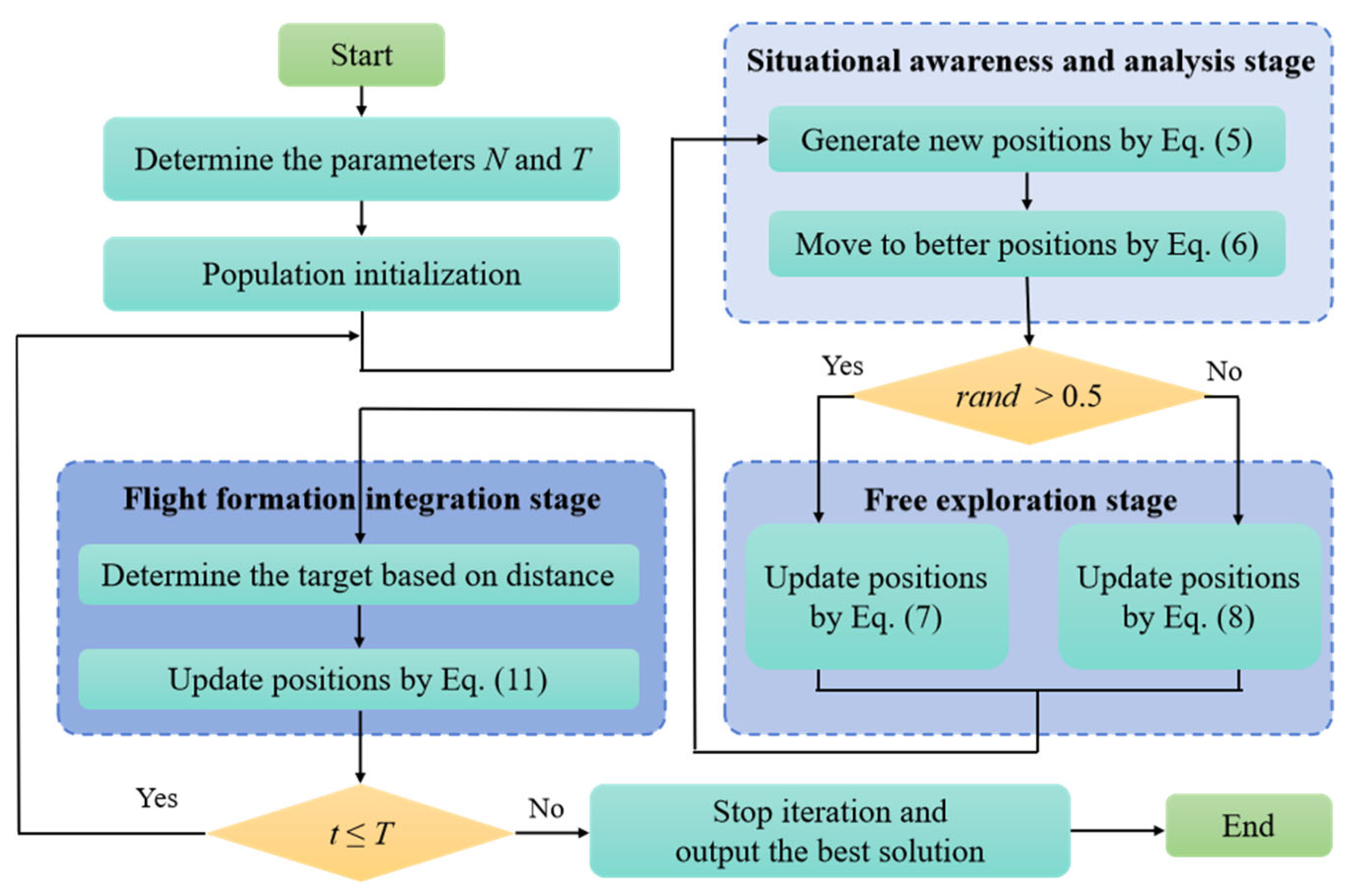
3.2. The Population Initialization Stage
3.3. Situational Awareness and Analysis Stage
3.4. Free Exploration Stage
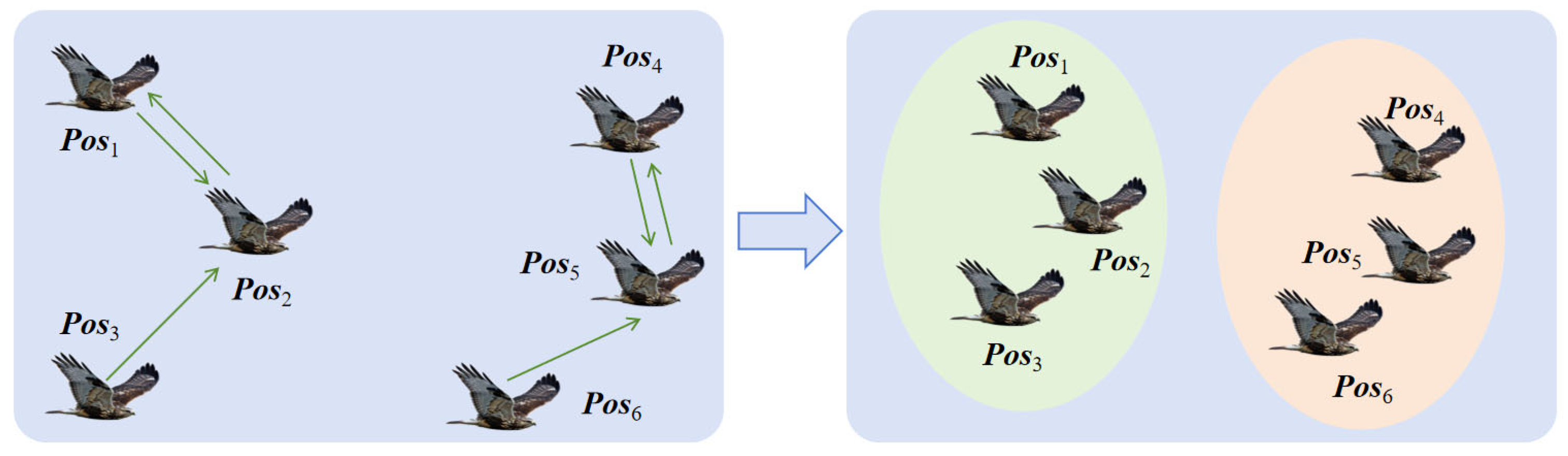
3.5. Flight Formation Integration Stage
4. Experimental Results and Analysis of the Proposed AEOA
4.1. Experimental Design and Comparison Algorithms
4.2. Quantitative Analysis
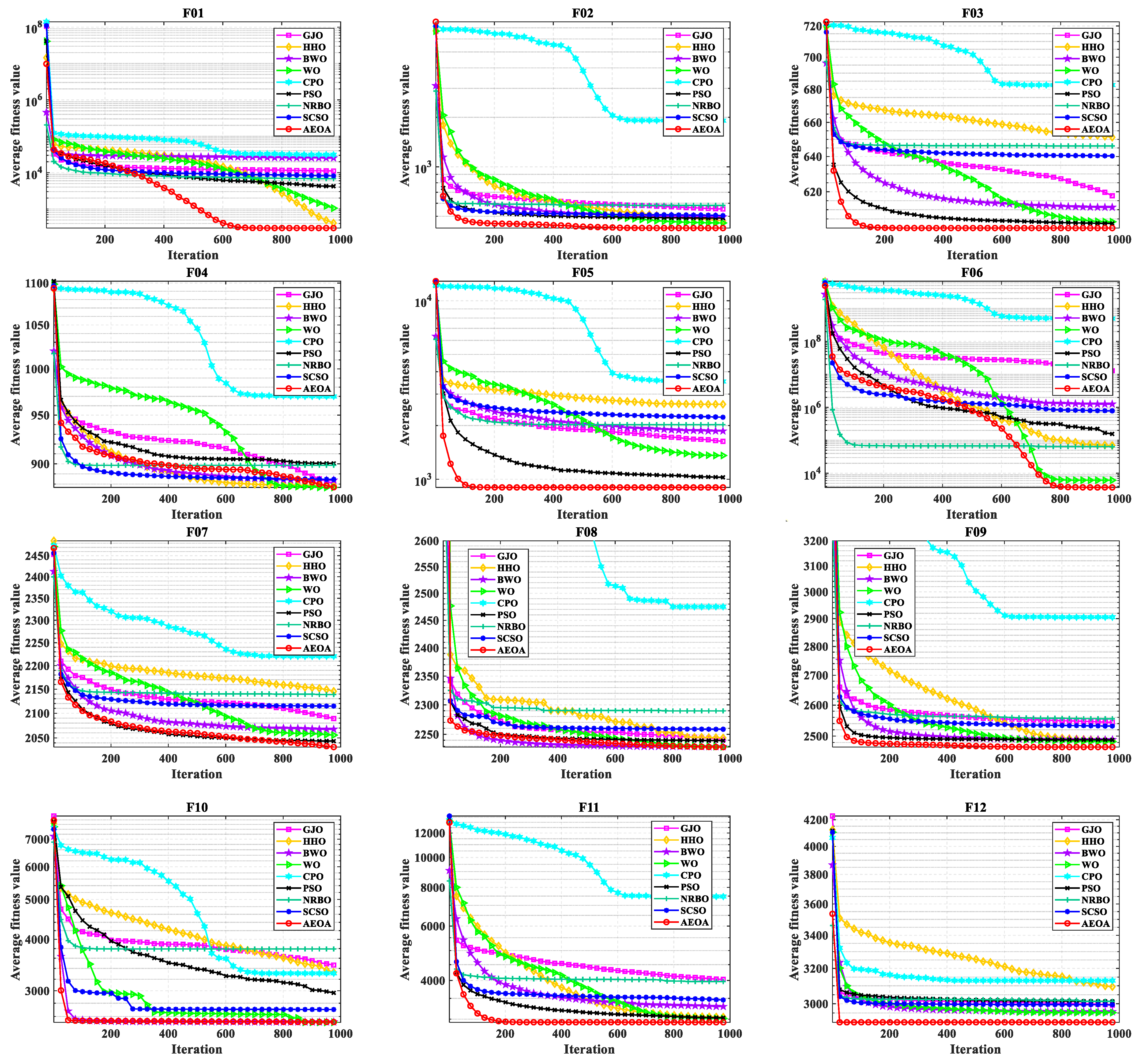
4.3. Convergence Analysis
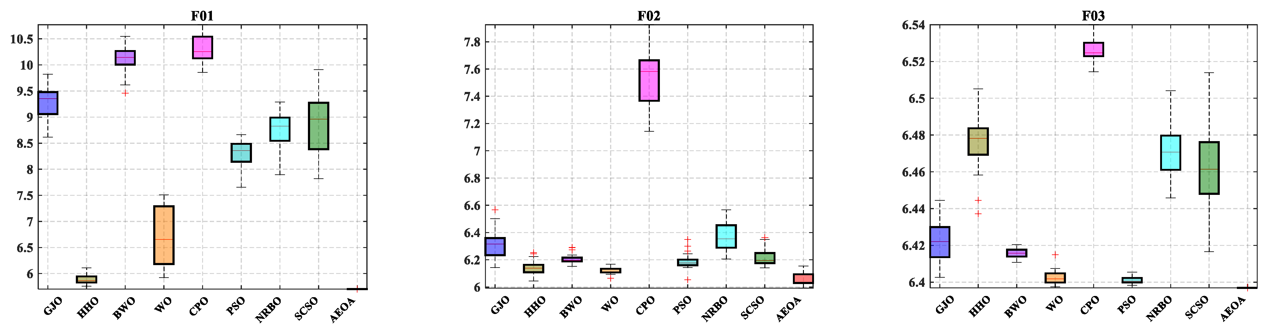
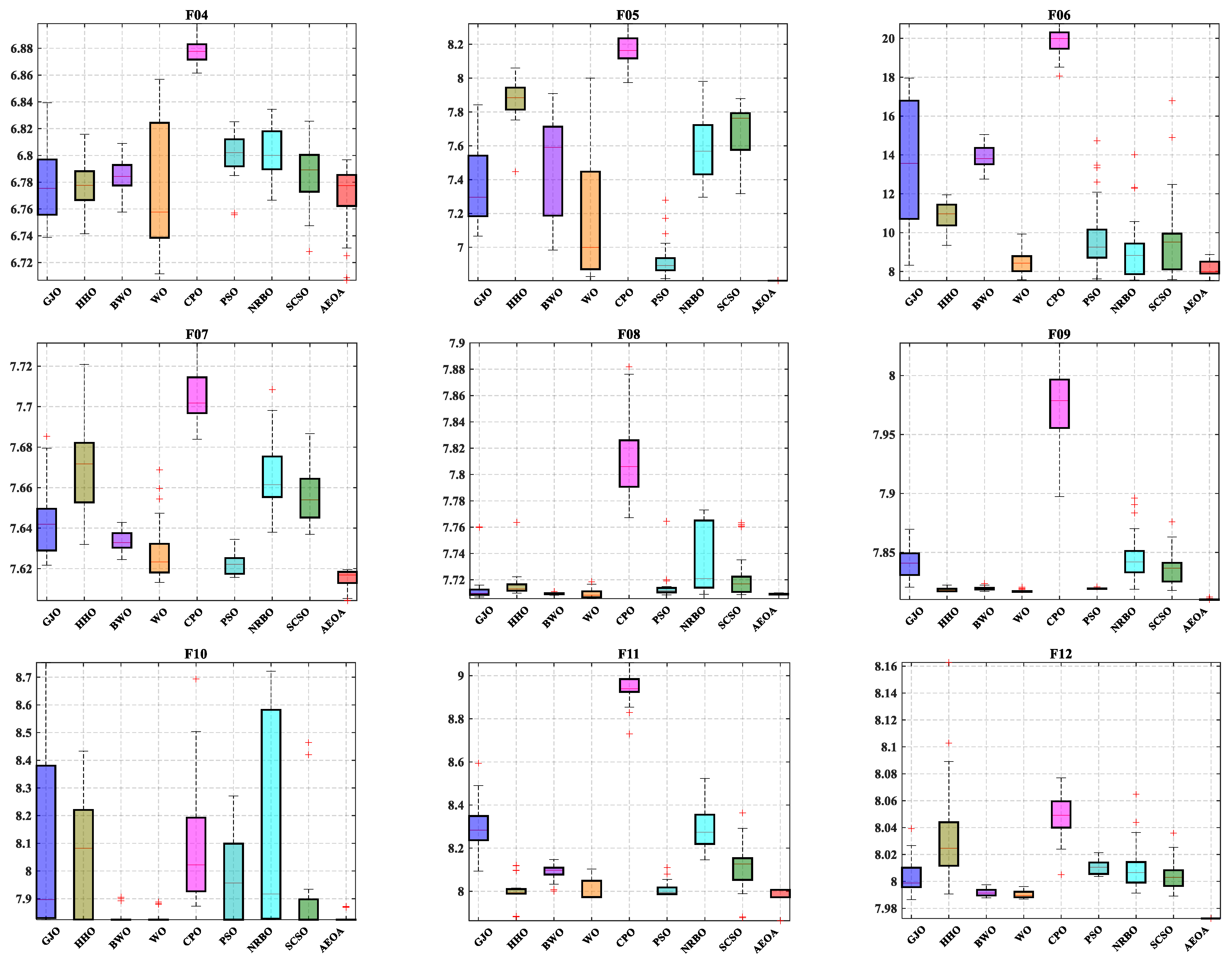
4.4. Stability Analysis
5. Trade Hub Location and Allocation Method Based on the AEOA
5.1. The Combination Between the Trade Hub Location and Allocation Model and the SEOA
5.2. Numerical Examples and Analysis
6. Conclusions and Future Work
Author Contributions
Funding
Institutional Review Board Statement
Informed Consent Statement
Data Availability Statement
Conflicts of Interest
Appendix A. The Iteration Curves and Boxplots of the AEOA and Other Comparison Algorithms
Appendix B. The Freight Between Different Towns in Case 1 and Case 2

| No. | 1 | 2 | 3 | 4 | 5 | 6 | 7 | 8 | 9 | 10 | 11 | 12 | 13 | 14 | 15 | 16 | 17 | 18 | 19 | 20 |
|---|---|---|---|---|---|---|---|---|---|---|---|---|---|---|---|---|---|---|---|---|
| 1 | 0 | 41 | 17 | 16 | 15 | 28 | 44 | 21 | 36 | 23 | 37 | 29 | 47 | 30 | 12 | 15 | 29 | 48 | 25 | 40 |
| 2 | 11 | 0 | 38 | 21 | 12 | 28 | 16 | 33 | 23 | 46 | 46 | 33 | 34 | 29 | 43 | 50 | 37 | 20 | 33 | 25 |
| 3 | 46 | 23 | 0 | 26 | 13 | 38 | 12 | 16 | 49 | 25 | 49 | 16 | 27 | 15 | 42 | 50 | 16 | 27 | 36 | 16 |
| 4 | 15 | 47 | 17 | 0 | 22 | 18 | 32 | 48 | 24 | 50 | 27 | 15 | 30 | 22 | 16 | 27 | 48 | 50 | 42 | 25 |
| 5 | 29 | 20 | 25 | 24 | 0 | 30 | 15 | 28 | 25 | 40 | 28 | 15 | 10 | 35 | 17 | 14 | 31 | 16 | 35 | 49 |
| 6 | 44 | 16 | 36 | 39 | 22 | 0 | 24 | 41 | 31 | 17 | 15 | 33 | 44 | 38 | 17 | 21 | 11 | 42 | 16 | 36 |
| 7 | 48 | 10 | 45 | 13 | 14 | 36 | 0 | 41 | 24 | 29 | 37 | 32 | 16 | 50 | 49 | 42 | 47 | 12 | 25 | 47 |
| 8 | 48 | 29 | 30 | 47 | 33 | 21 | 22 | 0 | 33 | 36 | 48 | 44 | 35 | 17 | 21 | 44 | 35 | 19 | 47 | 50 |
| 9 | 36 | 13 | 10 | 46 | 24 | 14 | 39 | 46 | 0 | 16 | 24 | 35 | 50 | 39 | 39 | 14 | 32 | 21 | 31 | 43 |
| 10 | 40 | 27 | 45 | 14 | 29 | 22 | 50 | 15 | 31 | 0 | 47 | 36 | 22 | 43 | 23 | 21 | 11 | 38 | 37 | 12 |
| 11 | 24 | 37 | 22 | 33 | 18 | 28 | 48 | 50 | 23 | 29 | 0 | 31 | 44 | 47 | 24 | 38 | 17 | 28 | 13 | 10 |
| 12 | 34 | 37 | 47 | 45 | 32 | 42 | 14 | 31 | 15 | 45 | 12 | 0 | 31 | 27 | 14 | 15 | 30 | 17 | 41 | 41 |
| 13 | 25 | 28 | 21 | 44 | 30 | 43 | 49 | 43 | 12 | 21 | 20 | 32 | 0 | 20 | 14 | 19 | 18 | 15 | 20 | 40 |
| 14 | 11 | 33 | 14 | 13 | 35 | 49 | 47 | 29 | 19 | 36 | 40 | 22 | 24 | 0 | 23 | 22 | 42 | 13 | 41 | 49 |
| 15 | 13 | 36 | 29 | 19 | 27 | 43 | 24 | 20 | 40 | 24 | 49 | 41 | 19 | 49 | 0 | 28 | 22 | 45 | 36 | 24 |
| 16 | 50 | 44 | 26 | 25 | 13 | 22 | 31 | 25 | 41 | 16 | 50 | 40 | 26 | 21 | 31 | 0 | 17 | 29 | 13 | 26 |
| 17 | 44 | 13 | 23 | 26 | 40 | 17 | 15 | 12 | 14 | 45 | 48 | 23 | 50 | 49 | 19 | 15 | 0 | 45 | 25 | 23 |
| 18 | 45 | 47 | 15 | 26 | 15 | 46 | 32 | 13 | 33 | 23 | 40 | 48 | 15 | 33 | 36 | 45 | 49 | 0 | 48 | 43 |
| 19 | 18 | 31 | 49 | 42 | 50 | 20 | 42 | 39 | 43 | 22 | 49 | 26 | 19 | 10 | 24 | 45 | 30 | 31 | 0 | 46 |
| 20 | 37 | 23 | 38 | 45 | 45 | 18 | 10 | 23 | 19 | 27 | 46 | 23 | 21 | 30 | 40 | 44 | 22 | 16 | 13 | 0 |
| No. | 1 | 2 | 3 | 4 | 5 | 6 | 7 | 8 | 9 | 10 | 11 | 12 | 13 | 14 | 15 | 16 | 17 | 18 | 19 | 20 |
|---|---|---|---|---|---|---|---|---|---|---|---|---|---|---|---|---|---|---|---|---|
| 1 | 0 | 42 | 36 | 21 | 17 | 50 | 39 | 13 | 50 | 45 | 37 | 17 | 30 | 35 | 38 | 46 | 34 | 33 | 13 | 14 |
| 2 | 16 | 0 | 33 | 49 | 18 | 20 | 35 | 49 | 38 | 44 | 14 | 10 | 23 | 34 | 31 | 24 | 16 | 42 | 21 | 11 |
| 3 | 37 | 32 | 0 | 21 | 44 | 30 | 17 | 45 | 43 | 28 | 25 | 47 | 47 | 12 | 16 | 44 | 30 | 40 | 34 | 12 |
| 4 | 31 | 19 | 11 | 0 | 48 | 41 | 36 | 40 | 45 | 29 | 13 | 45 | 50 | 30 | 12 | 23 | 49 | 15 | 13 | 26 |
| 5 | 31 | 28 | 23 | 15 | 0 | 27 | 21 | 21 | 36 | 34 | 46 | 33 | 21 | 28 | 30 | 16 | 39 | 44 | 28 | 45 |
| 6 | 24 | 23 | 19 | 24 | 14 | 0 | 46 | 30 | 35 | 48 | 20 | 19 | 49 | 47 | 12 | 30 | 33 | 35 | 47 | 34 |
| 7 | 26 | 21 | 36 | 28 | 38 | 32 | 0 | 31 | 50 | 13 | 50 | 50 | 15 | 34 | 24 | 30 | 30 | 24 | 35 | 11 |
| 8 | 11 | 12 | 46 | 50 | 36 | 20 | 25 | 0 | 50 | 45 | 49 | 22 | 36 | 40 | 17 | 42 | 33 | 30 | 35 | 21 |
| 9 | 34 | 12 | 49 | 28 | 16 | 33 | 46 | 26 | 0 | 24 | 14 | 38 | 37 | 23 | 28 | 16 | 35 | 26 | 16 | 44 |
| 10 | 13 | 25 | 15 | 20 | 13 | 43 | 34 | 27 | 42 | 0 | 16 | 24 | 19 | 21 | 13 | 36 | 26 | 37 | 46 | 29 |
| 11 | 26 | 49 | 16 | 17 | 33 | 43 | 40 | 20 | 18 | 33 | 0 | 10 | 34 | 30 | 39 | 32 | 20 | 23 | 42 | 19 |
| 12 | 24 | 34 | 46 | 14 | 49 | 33 | 39 | 28 | 17 | 15 | 50 | 0 | 25 | 42 | 32 | 45 | 43 | 12 | 13 | 48 |
| 13 | 47 | 30 | 32 | 25 | 28 | 21 | 18 | 37 | 12 | 24 | 28 | 24 | 0 | 27 | 24 | 35 | 33 | 22 | 10 | 15 |
| 14 | 40 | 34 | 12 | 37 | 37 | 27 | 30 | 21 | 35 | 46 | 50 | 35 | 10 | 0 | 20 | 31 | 31 | 44 | 48 | 16 |
| 15 | 10 | 41 | 32 | 16 | 10 | 13 | 50 | 30 | 48 | 20 | 25 | 38 | 26 | 45 | 0 | 42 | 39 | 44 | 14 | 37 |
| 16 | 37 | 12 | 11 | 15 | 22 | 38 | 35 | 44 | 50 | 34 | 15 | 12 | 49 | 39 | 41 | 0 | 49 | 15 | 11 | 32 |
| 17 | 14 | 19 | 45 | 42 | 28 | 42 | 15 | 41 | 24 | 19 | 12 | 41 | 42 | 13 | 12 | 14 | 0 | 41 | 36 | 46 |
| 18 | 20 | 13 | 46 | 40 | 24 | 10 | 23 | 44 | 50 | 17 | 46 | 25 | 47 | 19 | 31 | 41 | 25 | 0 | 26 | 28 |
| 19 | 27 | 40 | 18 | 17 | 39 | 44 | 24 | 14 | 14 | 16 | 20 | 35 | 14 | 22 | 40 | 40 | 48 | 26 | 0 | 30 |
| 20 | 13 | 31 | 39 | 23 | 17 | 18 | 47 | 14 | 34 | 13 | 45 | 13 | 14 | 14 | 48 | 31 | 17 | 21 | 39 | 0 |
| No. | 21 | 22 | 23 | 24 | 25 | 26 | 27 | 28 | 29 | 30 | 31 | 32 | 33 | 34 | 35 | 36 | 37 | 38 | 39 | 40 |
| 1 | 14 | 50 | 47 | 22 | 27 | 26 | 48 | 45 | 38 | 37 | 22 | 20 | 47 | 16 | 40 | 19 | 22 | 36 | 20 | 22 |
| 2 | 27 | 20 | 39 | 15 | 32 | 43 | 47 | 20 | 19 | 49 | 16 | 21 | 14 | 39 | 10 | 34 | 27 | 27 | 39 | 47 |
| 3 | 38 | 43 | 18 | 47 | 10 | 24 | 33 | 49 | 17 | 37 | 33 | 39 | 28 | 28 | 18 | 10 | 16 | 44 | 17 | 37 |
| 4 | 17 | 47 | 45 | 10 | 44 | 50 | 48 | 20 | 43 | 40 | 28 | 44 | 38 | 34 | 37 | 15 | 24 | 27 | 28 | 41 |
| 5 | 44 | 36 | 19 | 28 | 18 | 32 | 27 | 45 | 45 | 14 | 36 | 44 | 37 | 50 | 21 | 12 | 31 | 12 | 34 | 16 |
| 6 | 38 | 45 | 38 | 32 | 41 | 17 | 19 | 32 | 38 | 16 | 30 | 26 | 13 | 12 | 26 | 19 | 14 | 48 | 14 | 44 |
| 7 | 35 | 10 | 26 | 24 | 27 | 46 | 41 | 18 | 39 | 47 | 26 | 32 | 39 | 25 | 45 | 13 | 29 | 24 | 23 | 45 |
| 8 | 17 | 30 | 26 | 36 | 35 | 50 | 48 | 10 | 21 | 20 | 33 | 12 | 50 | 38 | 15 | 27 | 40 | 41 | 37 | 46 |
| 9 | 47 | 47 | 33 | 39 | 41 | 41 | 11 | 18 | 47 | 34 | 13 | 39 | 48 | 37 | 15 | 32 | 50 | 10 | 11 | 15 |
| 10 | 35 | 25 | 31 | 48 | 23 | 43 | 29 | 13 | 50 | 14 | 12 | 25 | 18 | 44 | 49 | 26 | 38 | 14 | 48 | 35 |
| 11 | 20 | 17 | 39 | 34 | 11 | 12 | 24 | 15 | 29 | 29 | 11 | 32 | 18 | 19 | 35 | 29 | 38 | 16 | 18 | 29 |
| 12 | 49 | 43 | 33 | 42 | 12 | 36 | 43 | 44 | 18 | 43 | 49 | 31 | 38 | 36 | 29 | 28 | 30 | 12 | 26 | 49 |
| 13 | 35 | 17 | 26 | 34 | 27 | 12 | 30 | 25 | 22 | 27 | 23 | 42 | 23 | 44 | 25 | 47 | 10 | 32 | 18 | 26 |
| 14 | 24 | 47 | 46 | 50 | 31 | 17 | 48 | 47 | 16 | 44 | 45 | 22 | 18 | 19 | 50 | 23 | 24 | 45 | 13 | 16 |
| 15 | 18 | 49 | 25 | 26 | 41 | 45 | 38 | 16 | 35 | 22 | 49 | 27 | 32 | 10 | 45 | 41 | 46 | 33 | 12 | 50 |
| 16 | 42 | 11 | 29 | 43 | 33 | 43 | 14 | 47 | 31 | 26 | 10 | 17 | 11 | 25 | 45 | 14 | 23 | 27 | 29 | 31 |
| 17 | 20 | 45 | 46 | 42 | 15 | 19 | 21 | 38 | 43 | 31 | 23 | 36 | 39 | 11 | 41 | 21 | 18 | 39 | 19 | 13 |
| 18 | 18 | 15 | 24 | 46 | 41 | 23 | 17 | 18 | 27 | 24 | 48 | 45 | 26 | 45 | 17 | 24 | 41 | 25 | 39 | 29 |
| 19 | 48 | 46 | 40 | 26 | 47 | 27 | 28 | 10 | 33 | 18 | 28 | 20 | 29 | 36 | 23 | 45 | 10 | 36 | 14 | 31 |
| 20 | 30 | 48 | 48 | 31 | 10 | 48 | 23 | 26 | 23 | 11 | 32 | 19 | 38 | 28 | 17 | 27 | 47 | 39 | 32 | 25 |
| No. | 1 | 2 | 3 | 4 | 5 | 6 | 7 | 8 | 9 | 10 | 11 | 12 | 13 | 14 | 15 | 16 | 17 | 18 | 19 | 20 |
| 21 | 14 | 50 | 47 | 22 | 27 | 26 | 48 | 45 | 38 | 37 | 22 | 20 | 47 | 16 | 40 | 19 | 22 | 36 | 20 | 22 |
| 22 | 27 | 20 | 39 | 15 | 32 | 43 | 47 | 20 | 19 | 49 | 16 | 21 | 14 | 39 | 10 | 34 | 27 | 27 | 39 | 47 |
| 23 | 38 | 43 | 18 | 47 | 10 | 24 | 33 | 49 | 17 | 37 | 33 | 39 | 28 | 28 | 18 | 10 | 16 | 44 | 17 | 37 |
| 24 | 17 | 47 | 45 | 10 | 44 | 50 | 48 | 20 | 43 | 40 | 28 | 44 | 38 | 34 | 37 | 15 | 24 | 27 | 28 | 41 |
| 25 | 44 | 36 | 19 | 28 | 18 | 32 | 27 | 45 | 45 | 14 | 36 | 44 | 37 | 50 | 21 | 12 | 31 | 12 | 34 | 16 |
| 26 | 38 | 45 | 38 | 32 | 41 | 17 | 19 | 32 | 38 | 16 | 30 | 26 | 13 | 12 | 26 | 19 | 14 | 48 | 14 | 44 |
| 27 | 35 | 10 | 26 | 24 | 27 | 46 | 41 | 18 | 39 | 47 | 26 | 32 | 39 | 25 | 45 | 13 | 29 | 24 | 23 | 45 |
| 28 | 17 | 30 | 26 | 36 | 35 | 50 | 48 | 10 | 21 | 20 | 33 | 12 | 50 | 38 | 15 | 27 | 40 | 41 | 37 | 46 |
| 29 | 47 | 47 | 33 | 39 | 41 | 41 | 11 | 18 | 47 | 34 | 13 | 39 | 48 | 37 | 15 | 32 | 50 | 10 | 11 | 15 |
| 30 | 35 | 25 | 31 | 48 | 23 | 43 | 29 | 13 | 50 | 14 | 12 | 25 | 18 | 44 | 49 | 26 | 38 | 14 | 48 | 35 |
| 31 | 20 | 17 | 39 | 34 | 11 | 12 | 24 | 15 | 29 | 29 | 11 | 32 | 18 | 19 | 35 | 29 | 38 | 16 | 18 | 29 |
| 32 | 49 | 43 | 33 | 42 | 12 | 36 | 43 | 44 | 18 | 43 | 49 | 31 | 38 | 36 | 29 | 28 | 30 | 12 | 26 | 49 |
| 33 | 35 | 17 | 26 | 34 | 27 | 12 | 30 | 25 | 22 | 27 | 23 | 42 | 23 | 44 | 25 | 47 | 10 | 32 | 18 | 26 |
| 34 | 24 | 47 | 46 | 50 | 31 | 17 | 48 | 47 | 16 | 44 | 45 | 22 | 18 | 19 | 50 | 23 | 24 | 45 | 13 | 16 |
| 35 | 18 | 49 | 25 | 26 | 41 | 45 | 38 | 16 | 35 | 22 | 49 | 27 | 32 | 10 | 45 | 41 | 46 | 33 | 12 | 50 |
| 36 | 42 | 11 | 29 | 43 | 33 | 43 | 14 | 47 | 31 | 26 | 10 | 17 | 11 | 25 | 45 | 14 | 23 | 27 | 29 | 31 |
| 37 | 20 | 45 | 46 | 42 | 15 | 19 | 21 | 38 | 43 | 31 | 23 | 36 | 39 | 11 | 41 | 21 | 18 | 39 | 19 | 13 |
| 38 | 18 | 15 | 24 | 46 | 41 | 23 | 17 | 18 | 27 | 24 | 48 | 45 | 26 | 45 | 17 | 24 | 41 | 25 | 39 | 29 |
| 39 | 48 | 46 | 40 | 26 | 47 | 27 | 28 | 10 | 33 | 18 | 28 | 20 | 29 | 36 | 23 | 45 | 10 | 36 | 14 | 31 |
| 40 | 30 | 48 | 48 | 31 | 10 | 48 | 23 | 26 | 23 | 11 | 32 | 19 | 38 | 28 | 17 | 27 | 47 | 39 | 32 | 25 |
| No. | 21 | 22 | 23 | 24 | 25 | 26 | 27 | 28 | 29 | 30 | 31 | 32 | 33 | 34 | 35 | 36 | 37 | 38 | 39 | 40 |
| 21 | 0 | 27 | 47 | 42 | 18 | 23 | 39 | 22 | 41 | 24 | 25 | 25 | 17 | 50 | 11 | 10 | 32 | 47 | 46 | 36 |
| 22 | 25 | 0 | 36 | 40 | 15 | 20 | 45 | 48 | 12 | 15 | 47 | 19 | 17 | 14 | 50 | 12 | 22 | 36 | 19 | 23 |
| 23 | 18 | 27 | 0 | 20 | 31 | 24 | 11 | 24 | 46 | 45 | 42 | 33 | 21 | 10 | 27 | 35 | 24 | 47 | 10 | 30 |
| 24 | 43 | 40 | 29 | 0 | 26 | 41 | 26 | 41 | 47 | 15 | 21 | 38 | 28 | 31 | 50 | 13 | 26 | 15 | 31 | 49 |
| 25 | 29 | 49 | 42 | 23 | 0 | 26 | 47 | 30 | 40 | 21 | 14 | 43 | 40 | 48 | 31 | 47 | 49 | 39 | 34 | 12 |
| 26 | 17 | 22 | 13 | 26 | 15 | 0 | 41 | 24 | 49 | 22 | 35 | 42 | 29 | 37 | 47 | 22 | 15 | 38 | 21 | 36 |
| 27 | 45 | 32 | 50 | 43 | 36 | 12 | 0 | 13 | 41 | 42 | 28 | 18 | 16 | 39 | 41 | 37 | 45 | 45 | 48 | 43 |
| 28 | 48 | 49 | 16 | 39 | 33 | 26 | 19 | 0 | 27 | 21 | 30 | 41 | 10 | 50 | 28 | 10 | 11 | 36 | 22 | 43 |
| 29 | 29 | 35 | 11 | 16 | 37 | 50 | 22 | 48 | 0 | 17 | 41 | 35 | 10 | 20 | 31 | 11 | 11 | 41 | 26 | 12 |
| 30 | 49 | 14 | 31 | 17 | 50 | 33 | 14 | 30 | 34 | 0 | 25 | 49 | 48 | 22 | 17 | 30 | 25 | 26 | 20 | 45 |
| 31 | 28 | 16 | 50 | 32 | 48 | 38 | 40 | 43 | 22 | 28 | 0 | 34 | 10 | 15 | 33 | 18 | 27 | 47 | 40 | 15 |
| 32 | 32 | 38 | 44 | 19 | 28 | 13 | 17 | 42 | 15 | 36 | 31 | 0 | 20 | 33 | 41 | 46 | 40 | 21 | 32 | 26 |
| 33 | 28 | 47 | 39 | 24 | 45 | 12 | 38 | 24 | 36 | 24 | 22 | 29 | 0 | 31 | 35 | 23 | 25 | 10 | 36 | 20 |
| 34 | 35 | 16 | 39 | 15 | 27 | 27 | 34 | 31 | 38 | 25 | 49 | 50 | 41 | 0 | 19 | 29 | 19 | 27 | 29 | 22 |
| 35 | 16 | 47 | 20 | 48 | 32 | 47 | 41 | 16 | 40 | 17 | 18 | 23 | 31 | 48 | 0 | 45 | 14 | 13 | 13 | 23 |
| 36 | 39 | 18 | 40 | 18 | 32 | 11 | 41 | 48 | 10 | 47 | 48 | 16 | 48 | 42 | 17 | 0 | 13 | 10 | 38 | 10 |
| 37 | 40 | 24 | 22 | 17 | 23 | 30 | 30 | 21 | 35 | 24 | 28 | 40 | 40 | 12 | 28 | 10 | 0 | 24 | 49 | 29 |
| 38 | 22 | 37 | 26 | 37 | 36 | 33 | 33 | 39 | 24 | 10 | 13 | 49 | 43 | 37 | 43 | 43 | 42 | 0 | 36 | 44 |
| 39 | 29 | 48 | 15 | 27 | 37 | 40 | 50 | 44 | 27 | 16 | 27 | 27 | 43 | 32 | 26 | 31 | 44 | 29 | 0 | 15 |
| 40 | 11 | 17 | 31 | 23 | 43 | 17 | 23 | 45 | 31 | 28 | 39 | 24 | 22 | 12 | 47 | 23 | 21 | 34 | 46 | 0 |
References
- Farahani, R.Z.; Hekmatfar, M.; Arabani, A.B.; Nikbakhsh, E. Hub location problems: A review of models, classification, solution techniques, and applications. Comput. Ind. Eng. 2013, 64, 1096–1109. [Google Scholar] [CrossRef]
- Koutsoukis, N.C.; Manousakis, N.M.; Georgilakis, P.S.; Korres, G.N. Numerical observability method for optimal phasor measurement units placement using recursive Tabu search method. IET Gener. Transm. Distrib. 2013, 7, 347–356. [Google Scholar] [CrossRef]
- Rahimi, Y.; Torabi, S.A.; Tavakkoli-Moghaddam, R. A new robust-possibilistic reliable hub protection model with elastic demands and backup hubs under risk. Eng. Appl. Artif. Intell. 2019, 86, 68–82. [Google Scholar] [CrossRef]
- Danach, K.; Gelareh, S.; Neamatian Monemi, R. The capacitated single-allocation p-hub location routing problem: A Lagrangian relaxation and a hyper-heuristic approach. EURO J. Transp. Logist. 2019, 8, 597–631. [Google Scholar] [CrossRef]
- Rahmati, R.; Bashiri, M.; Nikzad, E.; Siadat, A. A two-stage robust hub location problem with accelerated Benders decomposition algorithm. Int. J. Prod. Res. 2022, 60, 5235–5257. [Google Scholar] [CrossRef]
- Theodorakatos, N.P.; Babu, R.; Theodoridis, C.A.; Moschoudis, A.P. Mathematical models for the single-channel and multi-channel PMU allocation problem and their solution algorithms. Algorithms 2024, 17, 191. [Google Scholar] [CrossRef]
- Pan, J.S.; Song, P.C.; Chu, S.C.; Peng, Y.J. Improved Compact Cuckoo Search Algorithm Applied to Location of Drone Logistics Hub. Mathematics. 2020, 8, 333. [Google Scholar] [CrossRef]
- Alumur, S.A.; Campbell, J.F.; Contreras, I.; Kara, B.Y.; Marianov, V.; O’Kelly, M.E. Perspectives on modeling hub location problems. Eur. J. Oper. Res. 2021, 291, 1–17. [Google Scholar] [CrossRef]
- Jahani, H.; Abbasi, B.; Sheu, J.B.; Klibi, W. Supply chain network design with financial considerations: A comprehensive review. Eur. J. Oper. Res. 2024, 312, 799–839. [Google Scholar] [CrossRef]
- Mishra, M.; Singh, S.P.; Gupta, M.P. Location of competitive facilities: A comprehensive review and future research agenda. Benchmarking Int. J. 2023, 30, 1171–1230. [Google Scholar] [CrossRef]
- Matos, T. Primal-dual algorithms for the Capacitated Single Allocation p-Hub Location Problem. Int. J. Hybrid Intell. Syst. 2022, 18, 1–17. [Google Scholar] [CrossRef]
- Rostami, B.; Kämmerling, N.; Naoum-Sawaya, J.; Buchheim, C.; Clausen, U. Stochastic single-allocation hub location. Eur. J. Oper. Res. 2021, 289, 1087–1106. [Google Scholar] [CrossRef]
- Zhang, X.; Dong, S.; Liu, Y. p-hub median location optimization of hub-and-spoke air transport networks in express enterprise. Concurr. Comput. Pract. Exp. 2019, 31, e4981. [Google Scholar] [CrossRef]
- Silva, M.R.; Cunha, C.B. A tabu search heuristic for the uncapacitated single allocation p-hub maximal covering problem. Eur. J. Oper. Res. 2017, 262, 954–965. [Google Scholar] [CrossRef]
- Theodorakatos, N.P.; Moschoudis, A.P.; Lytras, M.D.; Kantoutsis, K.T. Research on optimization procedure of PMU positioning problem achieving maximum observability based on heuristic algorithms. AIP Conf. Proc. 2023, 2872, 120032. [Google Scholar] [CrossRef]
- Singh, S.P.; Singh, S.P. A multi-objective PMU placement method in power system via binary gravitational search algorithm. Electr. Power Compon. Syst. 2017, 45, 1832–1845. [Google Scholar] [CrossRef]
- Rathore, H.; Nandi, S.; Pandey, P.; Singh, S.P. Diversification-based learning simulated annealing algorithm for hub location problems. Benchmarking Int. J. 2019, 26, 1995–2016. [Google Scholar] [CrossRef]
- Bhattacharjee, A.K.; Mukhopadhyay, A. An improved genetic algorithm with local refinement for solving hierarchical single-allocation hub median facility location problem. Soft Comput. 2023, 27, 1493–1509. [Google Scholar] [CrossRef]
- Hu, G.; Du, B.; Wang, X.; Wei, G. An enhanced black widow optimization algorithm for feature selection. Knowl.-Based Syst. 2022, 235, 107638. [Google Scholar] [CrossRef]
- Li, W.; Wang, G.G.; Gandomi, A.H. A Survey of Learning-Based Intelligent Optimization Algorithms. Arch. Comput. Methods Eng. 2021, 28, 3781–3799. [Google Scholar] [CrossRef]
- Hu, G.; Du, B.; Li, H.; Wang, X. Quadratic interpolation boosted black widow spider-inspired optimization algorithm with wavelet mutation. Math. Comput. Simulat. 2022, 200, 428–467. [Google Scholar] [CrossRef]
- Ramos-Figueroa, O.; Quiroz-Castellanos, M. An experimental approach to designing grouping genetic algorithms. Swarm Evol. Comput. 2024, 86, 101490. [Google Scholar] [CrossRef]
- Li, J.; Soradi-Zeid, S.; Yousefpour, A.; Pan, D. Improved differential evolution algorithm based convolutional neural network for emotional analysis of music data. Appl. Soft Comput. 2024, 153, 111262. [Google Scholar] [CrossRef]
- Freitas, D.; Lopes, L.G.; Morgado-Dias, F. Particle Swarm Optimisation: A historical review up to the current developments. Entropy 2020, 22, 362. [Google Scholar] [CrossRef] [PubMed]
- Ramasamy, S.; Koodalsamy, B.; Koodalsamy, C.; Veerayan, M.B. Realistic method for placement of phasor measurement units through optimization problem formulation with conflicting objectives. Electr. Power Compon. Syst. 2021, 49, 474–487. [Google Scholar] [CrossRef]
- Ahmadianfar, I.; Bozorg-Haddad, O.; Chu, X. Gradient-based optimizer: A new metaheuristic optimization algorithm. Inf. Sci. 2020, 540, 131–159. [Google Scholar] [CrossRef]
- Mirjalili, S.; Mirjalili, S.M.; Hatamlou, A. Multi-Verse Optimizer: A nature-inspired algorithm for global optimization. Neural Comput. Appl. 2016, 27, 495–513. [Google Scholar] [CrossRef]
- Li, M.; Xu, G.; Lai, Q.; Chen, J. A chaotic strategy-based quadratic Opposition-Based Learning adaptive variable-speed whale optimization algorithm. Math. Comput. Simul. 2022, 193, 71–99. [Google Scholar] [CrossRef]
- Chatterjee, A.; Ghoshal, S.P.; Mukherjee, V. Craziness-based PSO with wavelet mutation for transient performance augmentation of thermal system connected to grid. Expert Syst. Appl. 2011, 38, 7784–7794. [Google Scholar] [CrossRef]
- Wang, Z.; Chen, Y.; Ding, S.; Liang, D.; He, H. A novel particle swarm optimization algorithm with Lévy flight and orthogonal learning. Swarm Evol. Comput. 2022, 75, 101207. [Google Scholar] [CrossRef]
- Hu, G.; Du, B.; Wei, G. HG-SMA: Hierarchical guided slime mould algorithm for smooth path planning. Artif. Intell. Rev. 2023, 56, 9267–9327. [Google Scholar] [CrossRef]
- Lapshin, A.S.; Andreychev, A.V.; Alpeev, M.A.; Kuznetsov, V.A. Methods And Techniques For Making Artificial Nests For The Eagle Owl (Bubo Bubo, Strigiformes, Strigidae) In Order To Increase Its Population. Zool. Zhurnal 2022, 101, 349–354. [Google Scholar]
- Hu, G.; Huang, F.; Chen, K.; Wei, G. MNEARO: A meta swarm intelligence optimization algorithm for engineering applications. Comput. Methods Appl. Mech. Eng. 2024, 419, 116664. [Google Scholar] [CrossRef]
- Chopra, N.; Mohsin Ansari, M. Golden jackal optimization: A novel nature-inspired optimizer for engineering applications. Expert Syst. Appl. 2022, 198, 116924. [Google Scholar] [CrossRef]
- Heidari, A.A.; Mirjalili, S.; Fairs, H.; Aljarah, I.; Mafarja, M.; Chen, H. Harris hawks optimization: Algorithm and applications. Future Gener. Comput. Syst. 2019, 97, 849–872. [Google Scholar] [CrossRef]
- Zhong, C.; Li, G.; Meng, Z. Beluga whale optimization: A novel nature-inspired metaheuristic algorithm. Knowl.-Based Syst. 2022, 251, 109215. [Google Scholar] [CrossRef]
- Han, M.; Du, Z.; Yuen, K.F.; Zhu, H.; Li, Y.; Yuan, Q. Walrus optimizer: A novel nature-inspired metaheuristic algorithm. Expert Syst. Appl. 2024, 239, 122413. [Google Scholar] [CrossRef]
- Valencia-Rivera, G.H.; Benavides-Robles, M.T.; Vela Morales, A.; Amaya, I.; Cruz-Duarte, J.M.; Ortiz-Bayliss, J.C.; Avina-Cervantes, J.G. A systematic review of metaheuristic algorithms in electric power systems optimization. Appl. Soft Comput. 2024, 150, 111047. [Google Scholar] [CrossRef]
- Tijjani, S.; Ab Wahab, M.N.; Mohd Noor, M.H. An enhanced particle swarm optimization with position update for optimal feature selection. Expert Syst. Appl. 2024, 247, 123337. [Google Scholar] [CrossRef]
- Sowmya, R.; Premkumar, M.; Jangir, P. Newton-Raphson-based optimizer: A new population-based metaheuristic algorithm for continuous optimization problems. Eng. Appl. Artif. Intell. 2024, 128, 107532. [Google Scholar] [CrossRef]
- Seyyedabbasi, A.; Kiani, F. Sand Cat swarm optimization: A nature-inspired algorithm to solve global optimization problems. Eng. Comput. 2023, 39, 2627–2651. [Google Scholar] [CrossRef]
- Slowik, A.; Kwasnicka, H. Evolutionary algorithms and their applications to engineering problems. Neural Comput. Appl. 2020, 32, 12363–12379. [Google Scholar] [CrossRef]
- Dehghani, M.; Hubalovsky, S.; Trojovsky, P. Northern Goshawk Optimization: A New Swarm-Based Algorithm for Solving Optimization Problems. IEEE Access 2021, 9, 162059–162080. [Google Scholar] [CrossRef]
- Li, S.; Chen, H.; Wang, M.; Heidari, A.A.; Mirjalili, S. Slime mould algorithm: A new method for stochastic optimization. Future Gener. Comput. Syst. 2020, 111, 300–323. [Google Scholar] [CrossRef]


| No. | 1 | 2 | 3 | 4 | 5 | 6 | 7 | 8 | 9 |
|---|---|---|---|---|---|---|---|---|---|
| GDP | 78,795.89 | 2,145,416.32 | 1,108,794.96 | 410,598.65 | 2,440,393.39 | 564,480.53 | 939,284.29 | 309,354.95 | 2,785,204.99 |
| No. | 10 | 11 | 12 | 13 | 14 | 15 | 16 | 17 | 18 |
| GDP | 467,981.43 | 1,311,947.73 | 183,583.15 | 631,897.30 | 4,189,183.53 | 2,147,166.81 | 7,714,263.67 | 230,297.02 | 2,079,477.64 |
| No. | 19 | 20 | 21 | 22 | 23 | 24 | 25 | 26 | 27 |
| GDP | 3,423,367.91 | 3,522,491.11 | 5,050,760.14 | 371,172.59 | 5,209,690.02 | 1,870,662.40 | 581,030.78 | 273,566.57 | 391,078.38 |
| No. | 28 | 29 | 30 | 31 | 32 | 33 | 34 | 35 | 36 |
| GDP | 2,458,452.16 | 324,325.48 | 286,022.20 | 2,193,078.64 | 2,392,058.37 | 324,378.48 | 326,268.13 | 3,014,318.01 | 2,208,285.49 |
| Type | Functions | Description | Range | Dimension | fmin |
|---|---|---|---|---|---|
| Uni-modal | F01 | Shifted and Full Rotated Zakharov Function | [−100,100] | 20 | 300 |
| Multi-modal | F02 | Shifted and Full Rotated Rosenbrock’s Function | [−100,100] | 20 | 400 |
| F03 | Shifted and Full Rotated Rastrigin’s Function | [−100,100] | 20 | 600 | |
| F04 | Shifted and Full Rotated Non-Continuous Rastrigin’s Function | [−100,100] | 20 | 800 | |
| F05 | Shifted and Full Rotated Levy Function | [−100,100] | 20 | 900 | |
| Hybrid | F06 | Hybrid Function 1 (N = 3) | [−100,100] | 20 | 1800 |
| F07 | Hybrid Function 2 (N = 6) | [−100,100] | 20 | 2000 | |
| F08 | Hybrid Function 3 (N = 5) | [−100,100] | 20 | 2200 | |
| Composition | F09 | Composition Function 1 (N = 5) | [−100,100] | 20 | 2300 |
| F10 | Composition Function 2 (N = 4) | [−100,100] | 20 | 2400 | |
| F11 | Composition Function 3 (N = 5) | [−100,100] | 20 | 2600 | |
| F12 | Composition Function 4 (N = 6) | [−100,100] | 20 | 2700 |
| Algorithms | Parameters and Values |
|---|---|
| GJO | The constant c1 = 1.5. |
| HHO | The initial energy E0 = 2. |
| BWO | The probability of whale fall decreases from 0.1 to 0.05. |
| WO | Proportion of females p = 0.4. |
| CPO | Random step factor DC = 0.7. |
| PSO | Individual cognitive factor c1 = 2, social cognitive factor c2 = 2.5, acceleration weight w = 2. |
| NRBO | Deciding factor for trap avoidance operator DF = 0.6; |
| SCSO | The maximum sensitivity S = 2. |
| F | Index | GJO | HHO | BWO | WO | CPO | PSO | NRBO | SCSO | AEOA |
|---|---|---|---|---|---|---|---|---|---|---|
| 01 | Ave_f | 1.11 × 10⁴ | 3.61 × 10² | 2.53 × 10⁴ | 9.26 × 10² | 3.11 × 10⁴ | 4.16 × 10³ | 6.74 × 10³ | 8.13 × 10³ | 3.00 × 10² |
| Std_f | 3.00 × 10³ | 3.48 × 101 | 6.03 × 10³ | 4.80 × 10² | 8.13 × 10³ | 1.02 × 10³ | 1.99 × 10³ | 4.56 × 10³ | 6.32 × 10⁻⁴ | |
| Rank | 7 | 2 | 8 | 3 | 9 | 4 | 5 | 6 | 1 | |
| 02 | Ave_f | 5.52 × 10² | 4.66 × 10² | 4.96 × 10² | 4.55 × 10² | 1.91 × 10³ | 4.87 × 10² | 5.83 × 10² | 5.04 × 10² | 4.24 × 10² |
| Std_f | 5.32 × 101 | 2.22 × 101 | 1.80 × 101 | 1.20 × 101 | 3.81 × 10² | 2.63 × 101 | 5.80 × 101 | 3.38 × 101 | 1.86 × 101 | |
| Rank | 7 | 3 | 5 | 2 | 9 | 4 | 8 | 6 | 1 | |
| 03 | Ave_f | 6.15 × 10² | 6.50 × 10² | 6.11 × 10² | 6.03 × 10² | 6.83 × 10² | 6.02 × 10² | 6.46 × 10² | 6.40 × 10² | 6.00 × 10² |
| Std_f | 6.20 × 10 | 9.77 × 10 | 1.54 × 10 | 2.21 × 10 | 4.27 × 10 | 1.09 × 10 | 9.52 × 10 | 1.50 × 101 | 3.55 × 10⁻² | |
| Rank | 5 | 8 | 4 | 3 | 9 | 2 | 7 | 6 | 1 | |
| 04 | Ave_f | 8.79 × 10² | 8.78 × 10² | 8.84 × 10² | 8.77 × 10² | 9.70 × 10² | 8.99 × 10² | 8.98 × 10² | 8.84 × 10² | 8.72 × 10² |
| Std_f | 2.24 × 101 | 1.43 × 101 | 1.04 × 101 | 4.02 × 101 | 8.99 × 10 | 1.50 × 101 | 1.66 × 101 | 1.97 × 101 | 2.01 × 101 | |
| Rank | 4 | 3 | 5 | 2 | 9 | 8 | 7 | 6 | 1 | |
| 05 | Ave_f | 1.61 × 10³ | 2.63 × 10³ | 1.86 × 10³ | 1.36 × 10³ | 3.53 × 10³ | 1.02 × 10³ | 2.02 × 10³ | 2.21 × 10³ | 9.00 × 10² |
| Std_f | 3.87 × 10² | 2.67 × 10² | 5.22 × 10² | 5.44 × 10² | 2.99 × 10² | 1.15 × 10² | 3.80 × 10² | 3.05 × 10² | 3.23 × 10⁻¹ | |
| Rank | 4 | 8 | 5 | 3 | 9 | 2 | 6 | 7 | 1 | |
| 06 | Ave_f | 1.24 × 10⁷ | 6.52 × 10⁴ | 1.26 × 10⁶ | 6.15 × 10³ | 4.92 × 10⁸ | 1.55 × 10⁵ | 6.33 × 10⁴ | 7.77 × 10⁵ | 3.72 × 10³ |
| Std_f | 1.94 × 10⁷ | 3.93 × 10⁴ | 7.28 × 10⁵ | 4.89 × 10³ | 2.46 × 10⁸ | 4.77 × 10⁵ | 2.25 × 10⁵ | 3.59 × 10⁶ | 1.68 × 10³ | |
| Rank | 8 | 4 | 7 | 2 | 9 | 5 | 3 | 6 | 1 | |
| 07 | Ave_f | 2.08 × 10³ | 2.14 × 10³ | 2.07 × 10³ | 2.06 × 10³ | 2.22 × 10³ | 2.04 × 10³ | 2.14 × 10³ | 2.11 × 10³ | 2.03 × 10³ |
| Std_f | 3.38 × 101 | 4.61 × 101 | 9.51 × 10 | 2.88 × 101 | 2.66 × 101 | 9.73 × 10 | 3.69 × 101 | 3.08 × 101 | 7.75 × 10 | |
| Rank | 5 | 8 | 4 | 3 | 9 | 2 | 7 | 6 | 1 | |
| 08 | Ave_f | 2.24 × 10³ | 2.24 × 10³ | 2.23 × 10³ | 2.23 × 10³ | 2.48 × 10³ | 2.24 × 10³ | 2.29 × 10³ | 2.26 × 10³ | 2.23 × 10³ |
| Std_f | 2.93 × 101 | 2.22 × 101 | 1.30 × 10 | 7.56 × 10 | 9.84 × 101 | 2.27 × 101 | 5.98 × 101 | 3.87 × 101 | 9.67 × 10⁻¹ | |
| Rank | 4 | 6 | 3 | 2 | 9 | 5 | 8 | 7 | 1 | |
| 09 | Ave_f | 2.54 × 10³ | 2.49 × 10³ | 2.49 × 10³ | 2.48 × 10³ | 2.91 × 10³ | 2.49 × 10³ | 2.55 × 10³ | 2.53 × 10³ | 2.47 × 10³ |
| Std_f | 3.06 × 101 | 4.12 × 10 | 3.53 × 10 | 2.56 × 10 | 9.06 × 101 | 1.10 × 10 | 4.95 × 101 | 3.62 × 101 | 9.86 × 10⁻¹ | |
| Rank | 7 | 3 | 5 | 2 | 9 | 4 | 8 | 6 | 1 | |
| 10 | Ave_f | 3.45 × 10³ | 3.23 × 10³ | 2.52 × 10³ | 2.52 × 10³ | 3.31 × 10³ | 2.95 × 10³ | 3.79 × 10³ | 2.70 × 10³ | 2.52 × 10³ |
| Std_f | 1.28 × 10³ | 6.81 × 10² | 5.93 × 101 | 4.65 × 101 | 7.75 × 10² | 4.57 × 10² | 1.47 × 10³ | 5.36 × 10² | 4.41 × 101 | |
| Rank | 8 | 6 | 3 | 1 | 7 | 5 | 9 | 4 | 2 | |
| 11 | Ave_f | 4.06 × 10³ | 3.00 × 10³ | 3.26 × 10³ | 3.01 × 10³ | 7.68 × 10³ | 3.01 × 10³ | 4.02 × 10³ | 3.35 × 10³ | 2.91 × 10³ |
| Std_f | 4.45 × 10² | 1.56 × 10² | 1.11 × 10² | 1.59 × 10² | 5.30 × 10² | 9.38 × 101 | 4.29 × 10² | 3.59 × 10² | 9.73 × 101 | |
| Rank | 8 | 2 | 5 | 4 | 9 | 3 | 7 | 6 | 1 | |
| 12 | Ave_f | 2.99 × 10³ | 3.09 × 10³ | 2.96 × 10³ | 2.95 × 10³ | 3.13 × 10³ | 3.01 × 10³ | 3.01 × 10³ | 2.99 × 10³ | 2.90 × 10³ |
| Std_f | 3.61 × 101 | 1.19 × 10² | 8.12 × 10 | 7.81 × 10 | 4.93 × 101 | 1.56 × 101 | 5.12 × 101 | 3.33 × 101 | 1.57 × 10⁻⁴ | |
| Rank | 4 | 8 | 3 | 2 | 9 | 6 | 7 | 5 | 1 | |
| Average rank | 5.917 | 5.083 | 4.750 | 2.417 | 8.833 | 4.167 | 6.833 | 5.917 | 1.083 | |
| Final rank | 6 | 5 | 4 | 2 | 9 | 3 | 8 | 6 | 1 | |
| CEC | GJO | HHO | BWO | WO | CPO | PSO | NRBO | SCSO |
|---|---|---|---|---|---|---|---|---|
| 01 | 3.02 × 10⁻¹¹/+ | 3.02 × 10⁻¹¹/+ | 3.02 × 10⁻¹¹/+ | 3.02 × 10⁻¹¹/+ | 3.02 × 10⁻¹¹/+ | 3.02 × 10⁻¹¹/+ | 3.02 × 10⁻¹¹/+ | 3.02 × 10⁻¹¹/+ |
| 02 | 3.34 × 10⁻¹¹/+ | 9.76 × 10⁻¹⁰/+ | 3.34 × 10⁻¹¹/+ | 2.03 × 10⁻⁹/+ | 3.02 × 10⁻¹¹/+ | 1.21 × 10⁻¹⁰/+ | 3.02 × 10⁻¹¹/+ | 4.08 × 10⁻¹¹/+ |
| 03 | 2.88 × 10⁻¹¹/+ | 2.88 × 10⁻¹¹/+ | 2.88 × 10⁻¹¹/+ | 2.88 × 10⁻¹¹/+ | 2.88 × 10⁻¹¹/+ | 2.88 × 10⁻¹¹/+ | 2.88 × 10⁻¹¹/+ | 2.88 × 10⁻¹¹/+ |
| 04 | 5.30 × 10⁻¹/= | 5.79 × 10⁻¹/= | 9.47 × 10⁻³/+ | 5.20 × 10⁻¹/= | 3.02 × 10⁻¹¹/+ | 3.65 × 10⁻⁸/+ | 8.84 × 10⁻⁷/+ | 7.29 × 10⁻³/+ |
| 05 | 3.02 × 10⁻¹¹/+ | 3.02 × 10⁻¹¹/+ | 3.02 × 10⁻¹¹/+ | 3.02 × 10⁻¹¹/+ | 3.02 × 10⁻¹¹/+ | 3.02 × 10⁻¹¹/+ | 3.02 × 10⁻¹¹/+ | 3.02 × 10⁻¹¹/+ |
| 06 | 1.61 × 10⁻¹⁰/+ | 3.02 × 10⁻¹¹/+ | 3.02 × 10⁻¹¹/+ | 2.92 × 10⁻²/+ | 3.02 × 10⁻¹¹/+ | 2.38 × 10⁻⁷/+ | 2.42 × 10⁻²/+ | 1.78 × 10⁻⁴/+ |
| 07 | 3.02 × 10⁻¹¹/+ | 3.02 × 10⁻¹¹/+ | 3.02 × 10⁻¹¹/+ | 2.15 × 10⁻⁶/+ | 3.02 × 10⁻¹¹/+ | 2.15 × 10⁻⁶/+ | 3.02 × 10⁻¹¹/+ | 3.02 × 10⁻¹¹/+ |
| 08 | 3.92 × 10⁻²/+ | 3.34 × 10⁻¹¹/+ | 3.67 × 10⁻³/+ | 1.45 × 10⁻¹/= | 3.02 × 10⁻¹¹/+ | 5.46 × 10⁻⁹/+ | 1.78 × 10⁻¹⁰/+ | 2.92 × 10⁻⁹/+ |
| 09 | 3.02 × 10⁻¹¹/+ | 3.02 × 10⁻¹¹/+ | 3.02 × 10⁻¹¹/+ | 3.02 × 10⁻¹¹/+ | 3.02 × 10⁻¹¹/+ | 3.02 × 10⁻¹¹/+ | 3.02 × 10⁻¹¹/+ | 3.02 × 10⁻¹¹/+ |
| 10 | 1.56 × 10⁻⁸/+ | 2.23 × 10⁻⁹/+ | 3.32 × 10⁻⁶/+ | 3.83 × 10⁻⁶/− | 3.02 × 10⁻¹¹/+ | 7.77 × 10⁻⁹/+ | 2.02 × 10⁻⁸/+ | 2.38 × 10⁻⁷/+ |
| 11 | 3.02 × 10⁻¹¹/+ | 1.78 × 10⁻⁴/+ | 8.15 × 10⁻¹¹/+ | 1.25 × 10⁻⁴/+ | 3.02 × 10⁻¹¹/+ | 2.25 × 10⁻⁴/+ | 3.02 × 10⁻¹¹/+ | 3.81 × 10⁻⁷/+ |
| 12 | 3.02 × 10⁻¹¹/+ | 3.02 × 10⁻¹¹/+ | 3.02 × 10⁻¹¹/+ | 3.02 × 10⁻¹¹/+ | 3.02 × 10⁻¹¹/+ | 3.02 × 10⁻¹¹/+ | 3.02 × 10⁻¹¹/+ | 3.02 × 10⁻¹¹/+ |
| +/=/− | 11/1/0 | 11/1/0 | 12/0/0 | 9/2/1 | 12/0/0 | 12/0/0 | 12/0/0 | 12/0/0 |
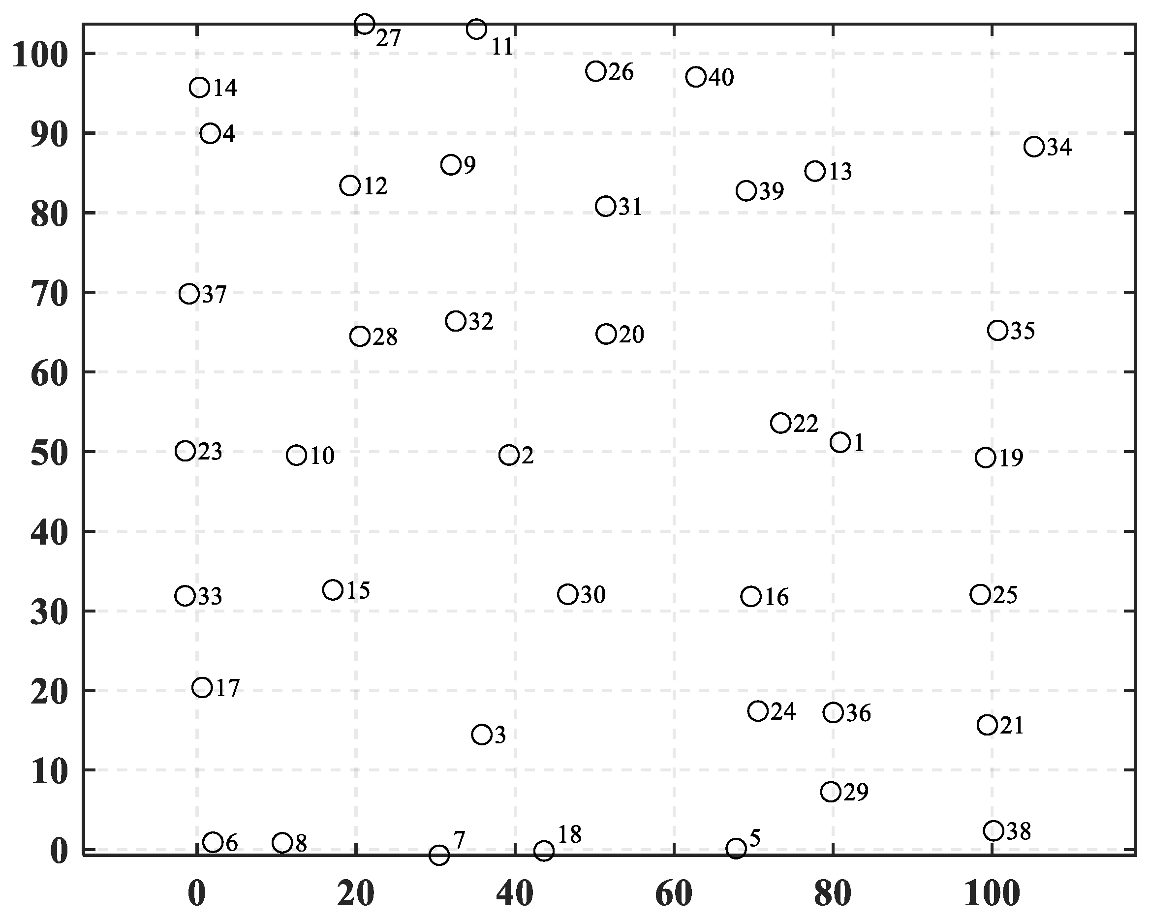
| No. | 1 | 2 | 3 | 4 | 5 | 6 | 7 | 8 | 9 | 10 | 11 | 12 | 13 | 14 | 15 | 16 | 17 | 18 | 19 | 20 |
|---|---|---|---|---|---|---|---|---|---|---|---|---|---|---|---|---|---|---|---|---|
| x | 69.5 | 53.7 | 19.2 | −0.3 | 48.4 | 52.7 | 2.0 | 71.8 | 98.9 | 79.4 | 69.9 | 99.9 | 1.4 | 29.0 | 44.6 | 2.6 | 95.7 | 107.5 | 53.5 | 3.5 |
| y | 98.1 | 69.8 | 5.3 | 18.1 | 28.2 | 48.5 | 44.6 | 54.6 | 99.8 | 17.7 | 1.7 | 51.5 | 5.3 | 21.9 | 94.5 | 77.1 | 29.0 | 73.6 | 5.3 | 100.9 |
| 1 | 2 | 3 | 4 | 5 | 6 | 7 | 8 | 9 | 10 | 11 | 12 | 13 | 14 | 15 | 16 | 17 | 18 | 19 | 20 | |
|---|---|---|---|---|---|---|---|---|---|---|---|---|---|---|---|---|---|---|---|---|
| AEOA | 8 | 6 | 5 | 5 | — | — | 5 | — | 8 | 5 | 5 | 8 | 5 | 5 | 6 | 6 | 8 | 8 | 5 | 6 |
| DE | 8 | 6 | 5 | 5 | — | — | 5 | — | 8 | 5 | 5 | 8 | 5 | 5 | 8 | 5 | 5 | 8 | 5 | 6 |
| NGO | 8 | 6 | 5 | 6 | — | — | 6 | — | 8 | 5 | 8 | 8 | 5 | 6 | 6 | 6 | 8 | 8 | 5 | 6 |
| SMA | 5 | — | 5 | — | — | 5 | 5 | 5 | 2 | 5 | 5 | 5 | 4 | 5 | 2 | 4 | 5 | 2 | 5 | 5 |
| Transportation Cost | Construction Cost | Fitness Value | |
|---|---|---|---|
| AEOA | 9,402,315.2 | 8,114,591 | 55,126,167 |
| DE | 9,638,692.8 | 8,114,591 | 56,308,055 |
| NGO | 9,862,185.6 | 8,114,591 | 57,425,519 |
| SMA | 10,388,245 | 7,212,142 | 59,153,367 |
| No. | 1 | 2 | 3 | 4 | 5 | 6 | 7 | 8 | 9 | 10 | 11 | 12 | 13 | 14 | 15 | 16 | 17 | 18 | 19 | 20 |
|---|---|---|---|---|---|---|---|---|---|---|---|---|---|---|---|---|---|---|---|---|
| x | 80.9 | 39.2 | 35.8 | 1.7 | 67.8 | 2.0 | 30.5 | 10.7 | 31.9 | 12.5 | 35.1 | 19.2 | 77.7 | 0.3 | 17.1 | 69.7 | 0.6 | 43.6 | 99.2 | 51.5 |
| y | 51.2 | 49.6 | 14.5 | 90.0 | 0.1 | 0.9 | −0.7 | 0.9 | 86.0 | 49.5 | 103.1 | 83.4 | 85.2 | 95.7 | 32.6 | 31.8 | 20.4 | −0.2 | 49.3 | 64.8 |
| No. | 21 | 22 | 23 | 24 | 25 | 26 | 27 | 28 | 29 | 30 | 31 | 32 | 33 | 34 | 35 | 36 | 37 | 38 | 39 | 40 |
| x | 99.4 | 73.4 | −1.5 | 70.5 | 98.5 | 50.2 | 21.1 | 20.5 | 79.7 | 46.6 | 51.4 | 32.5 | −1.5 | 105.3 | 100.7 | 80.0 | −1.0 | 100.2 | 69.1 | 62.7 |
| y | 15.7 | 53.6 | 50.1 | 17.4 | 32.1 | 97.8 | 103.7 | 64.5 | 7.3 | 32.1 | 80.8 | 66.4 | 31.9 | 88.3 | 65.2 | 17.2 | 69.8 | 2.4 | 82.8 | 97.1 |
| 1 | 2 | 3 | 4 | 5 | 6 | 7 | 8 | 9 | 10 | 11 | 12 | 13 | 14 | 15 | 16 | 17 | 18 | 19 | 20 | |
|---|---|---|---|---|---|---|---|---|---|---|---|---|---|---|---|---|---|---|---|---|
| AEOA | — | — | 16 | 28 | 24 | 2 | 2 | 2 | 32 | 28 | 32 | 32 | 20 | 28 | 2 | — | 2 | 24 | 1 | — |
| DE | 30 | — | 16 | 28 | 30 | 2 | 30 | 32 | 28 | 2 | 32 | 2 | 20 | 28 | 30 | — | 2 | 30 | 16 | — |
| NGO | 16 | — | 30 | 28 | 30 | 30 | 30 | 30 | 2 | — | 20 | 28 | 20 | 28 | 2 | — | 10 | 2 | 20 | — |
| SMA | 30 | 20 | 16 | 32 | 24 | 16 | 10 | 10 | 10 | — | — | 20 | 32 | 11 | 32 | — | 10 | 32 | 11 | — |
| 21 | 22 | 23 | 24 | 25 | 26 | 27 | 28 | 29 | 30 | 31 | 32 | 33 | 34 | 35 | 36 | 37 | 38 | 39 | 40 | |
| AEOA | 24 | 1 | 28 | — | 1 | 20 | 32 | — | 24 | 2 | 20 | — | 2 | 1 | 1 | 16 | 28 | 24 | 20 | 20 |
| DE | 16 | 2 | 28 | 30 | 16 | 20 | 28 | — | 16 | — | 2 | — | 28 | 28 | 2 | 2 | 28 | — | 16 | 28 |
| NGO | 16 | 20 | 10 | 16 | 16 | 2 | 28 | — | 16 | — | 2 | — | 10 | 20 | 16 | 16 | 32 | 16 | 20 | 2 |
| SMA | 20 | 32 | 20 | — | 24 | 20 | 30 | 10 | 24 | — | 20 | — | 30 | 30 | 20 | 24 | 30 | 30 | 30 | 32 |
| Transportation Cost | Construction Cost | Fitness Value | |
|---|---|---|---|
| AEOA | 34,451,386.4 | 27,773,090 | 200,030,000 |
| DE | 40,361,408.6 | 28,675,494 | 230,483,000 |
| NGO | 36,416,424.2 | 28,621,086 | 210,703,000 |
| SMA | 46,655,965.7 | 28,794,626 | 262,074,000 |
| No. | 1 | 2 | 3 | 4 | 5 | 6 | 7 | 8 | 9 | 10 | 11 | 12 | 13 | 14 | 15 | 16 | 17 | 18 |
|---|---|---|---|---|---|---|---|---|---|---|---|---|---|---|---|---|---|---|
| AEOA | — | 1 | 1 | 1 | 1 | 1 | 1 | 1 | 1 | 1 | 1 | 1 | 1 | 1 | 1 | 22 | 22 | 22 |
| No. | 19 | 20 | 21 | 22 | 23 | 24 | 25 | 26 | 27 | 28 | 29 | 30 | 31 | 32 | 33 | 34 | 35 | 36 |
| AEOA | 22 | 22 | 33 | — | 22 | 22 | 26 | — | 1 | 1 | 1 | 26 | 26 | 26 | — | 33 | 33 | 33 |
Disclaimer/Publisher’s Note: The statements, opinions and data contained in all publications are solely those of the individual author(s) and contributor(s) and not of MDPI and/or the editor(s). MDPI and/or the editor(s) disclaim responsibility for any injury to people or property resulting from any ideas, methods, instructions or products referred to in the content. |
© 2025 by the authors. Licensee MDPI, Basel, Switzerland. This article is an open access article distributed under the terms and conditions of the Creative Commons Attribution (CC BY) license (https://creativecommons.org/licenses/by/4.0/).
Share and Cite
Hu, S.; Hu, G.; Du, B.; Hussien, A.G. A Novel Artificial Eagle-Inspired Optimization Algorithm for Trade Hub Location and Allocation Method. Biomimetics 2025, 10, 481. https://doi.org/10.3390/biomimetics10080481
Hu S, Hu G, Du B, Hussien AG. A Novel Artificial Eagle-Inspired Optimization Algorithm for Trade Hub Location and Allocation Method. Biomimetics. 2025; 10(8):481. https://doi.org/10.3390/biomimetics10080481
Chicago/Turabian StyleHu, Shuhan, Gang Hu, Bo Du, and Abdelazim G. Hussien. 2025. "A Novel Artificial Eagle-Inspired Optimization Algorithm for Trade Hub Location and Allocation Method" Biomimetics 10, no. 8: 481. https://doi.org/10.3390/biomimetics10080481
APA StyleHu, S., Hu, G., Du, B., & Hussien, A. G. (2025). A Novel Artificial Eagle-Inspired Optimization Algorithm for Trade Hub Location and Allocation Method. Biomimetics, 10(8), 481. https://doi.org/10.3390/biomimetics10080481