
A Novel Exploration Stage Approach to Improve Crayfish Optimization Algorithm: Solution to Real-World Engineering Design Problems

Abstract

1. Introduction
- Global search: they could search the whole solution space effectively and discover the best fit solution for the problem.
- Scalability: they could be applied to high-dimensional, non-linear, and continuous or discrete problems.
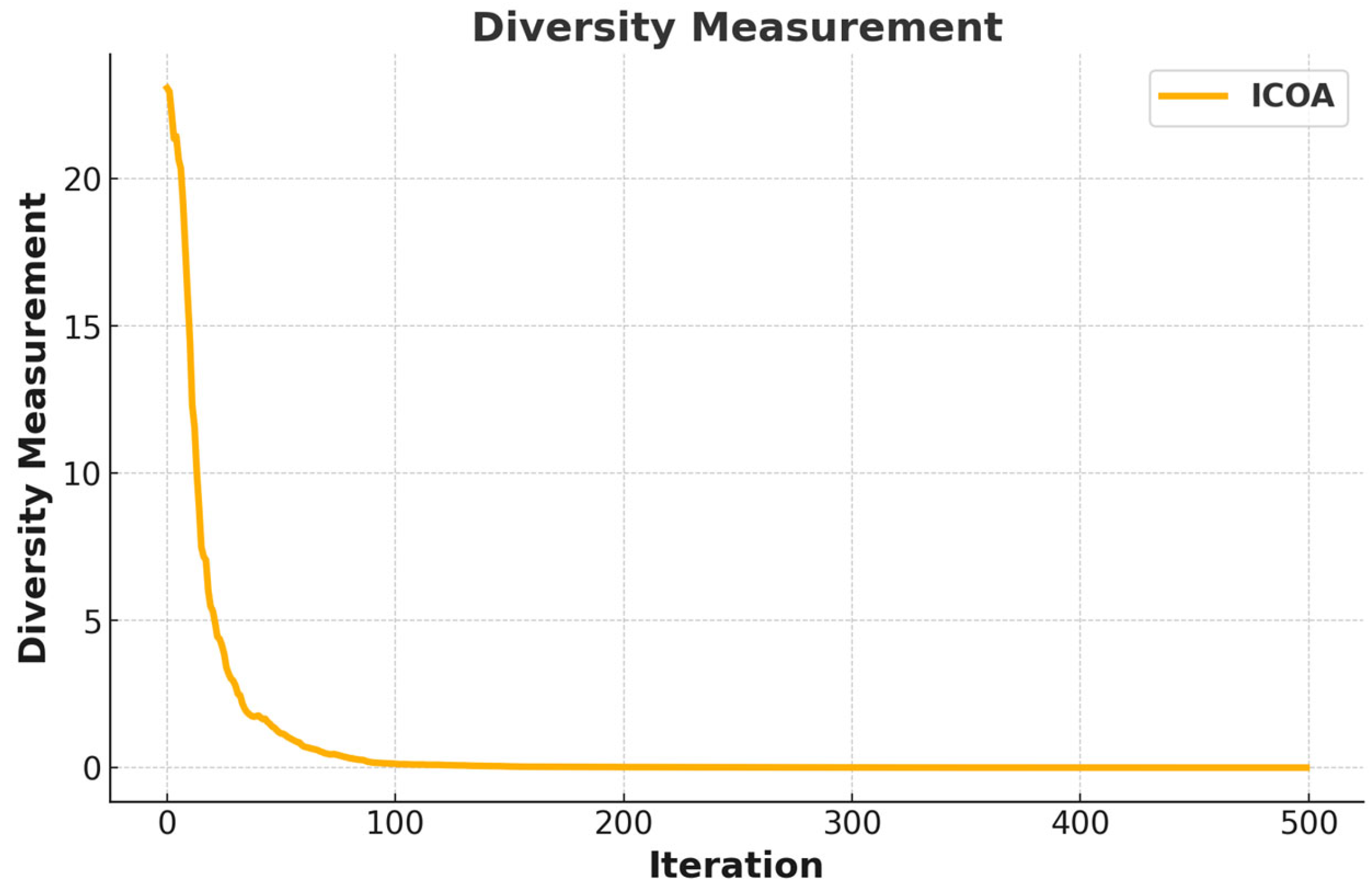
- Diversity: since the whole solution space is scanned in global search, population diversity is generated.
- Adaptability: MHAs could be applied to various problems in finance, economy, engineering, medicine, etc.
- Computational efficiency: MHAs generate acceptable results in a reasonable time. This property of MHAs presents them as advantageous compared to exact methods for the solution of high-scaled optimization problems.
- Gradient descent: MHAs do not need gradient descent information. Moreover, the mathematical models of MHAs are simple.
- At the competition stage of the COA, crayfish have to compete with the other crayfish in order to go in the cave. In the original COA, this competition is modeled only by distance. In the ICOA, besides the distance, the step length and locations of crayfish are added to the model.
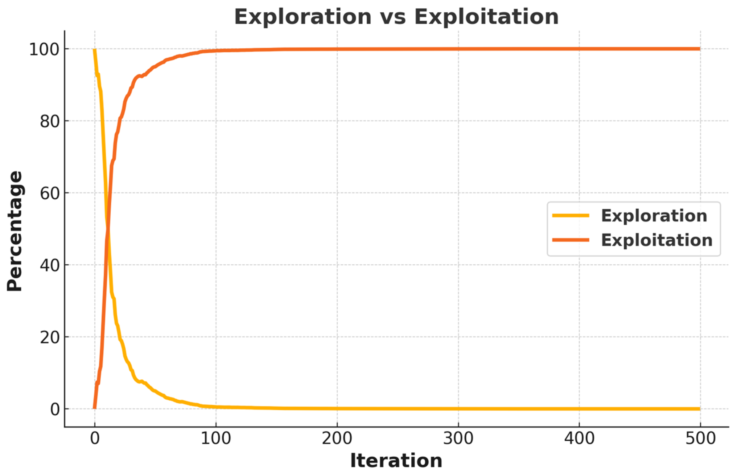
- The step length of crayfish differs depending on the iteration. Big steps are produced at low iteration numbers while at high iteration numbers, there occur small steps. Such a case allows the competition stage to help exploration at low iteration numbers and to help exploitation at high iteration numbers.
- In addition, at the competition stage of the ICOA, the cave location, which represents the best location, is removed from the mathematical model. The reason for that is to increase the exploration ability of the ICAO. Cave locations are also available in other stages.
- To verify the validity of the ICOA, it was compared to nine MHAs. For comparison, the CEC-2014 dataset with 30 test functions was used. Five engineering design problems were used for comparison as well.
- The results are interpreted by the Wilcoxon Signed-Rank Test and Friedman test.
2. Crayfish Optimization Algorithm (COA)
2.1. Define Temperature and Crayfish Intake
2.2. Summer Resort Stage (Exploration)
2.3. Competition Stage (Exploitation)
2.4. Foraging Stage (Exploitation)
3. Improved Crayfish Optimization Algorithm
| Algorithm 1. Pseudo-codes of algorithms. | |
| COA pseudo-code | ICOA pseudo-code |
| Input: T: maximum iteration, N: population size, D: variable dimension | Input: T: maximum iteration, N: population size, D: variable dimension |
| Output: The optimal search agent , and its fitness value | Output: The optimal search agent , and its fitness value |
| Generate initial population Calculate the fitness value of the population to get , Defining temperature temp by Equation (1) Define cave according to Equation (3) Crayfish conducts the summer resort stage according to Equation (4) Crayfish compete for caves through Equation (6) The food intake p and food size are obtained by Equation (2) and Equation (9) Crayfish shreds food by Equation (10) Crayfish foraging according to Equation (11) Crayfish foraging according to Equation (12) Update fitness values, , | Generate initial population Calculate the fitness value of the population to get , Defining temperature temp by Equation (1) Define cave according to Equation (3) Crayfish conducts the summer resort stage according to Equation (4) Updated competition stage Equation (13) The food intake p and food size are obtained by Equation (2) and Equation (9) Crayfish shreds food by Equation (10) Crayfish foraging according to Equation (11) Crayfish foraging according to Equation (12) Update fitness values, , |
4. Computational Results and Discussions
4.1. Experimental Settings and Compared Algorithms
4.2. CEC-2014 Benchmark Function Results
4.3. Ablation Study: Evidence of Component-Wise Improvements
4.4. Scalability Analysis
4.5. Application of ICOA to Engineering Problems
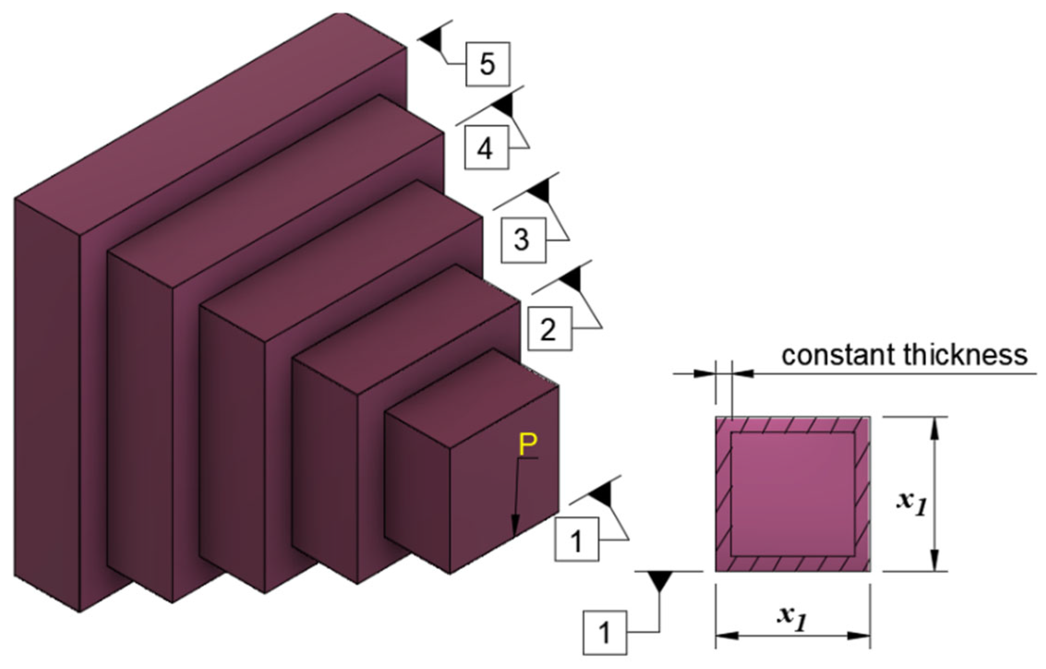
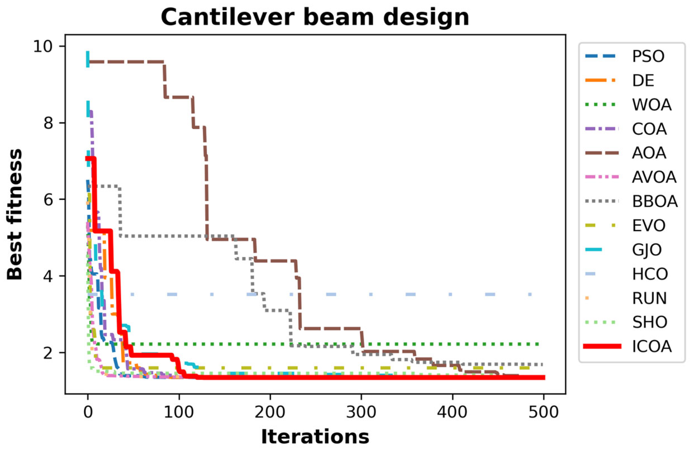
4.5.1. Cantilever Beam Design
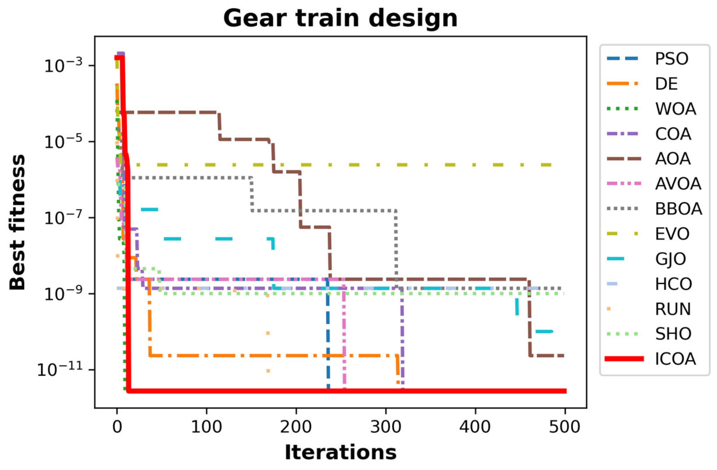
4.5.2. Gear Train Design
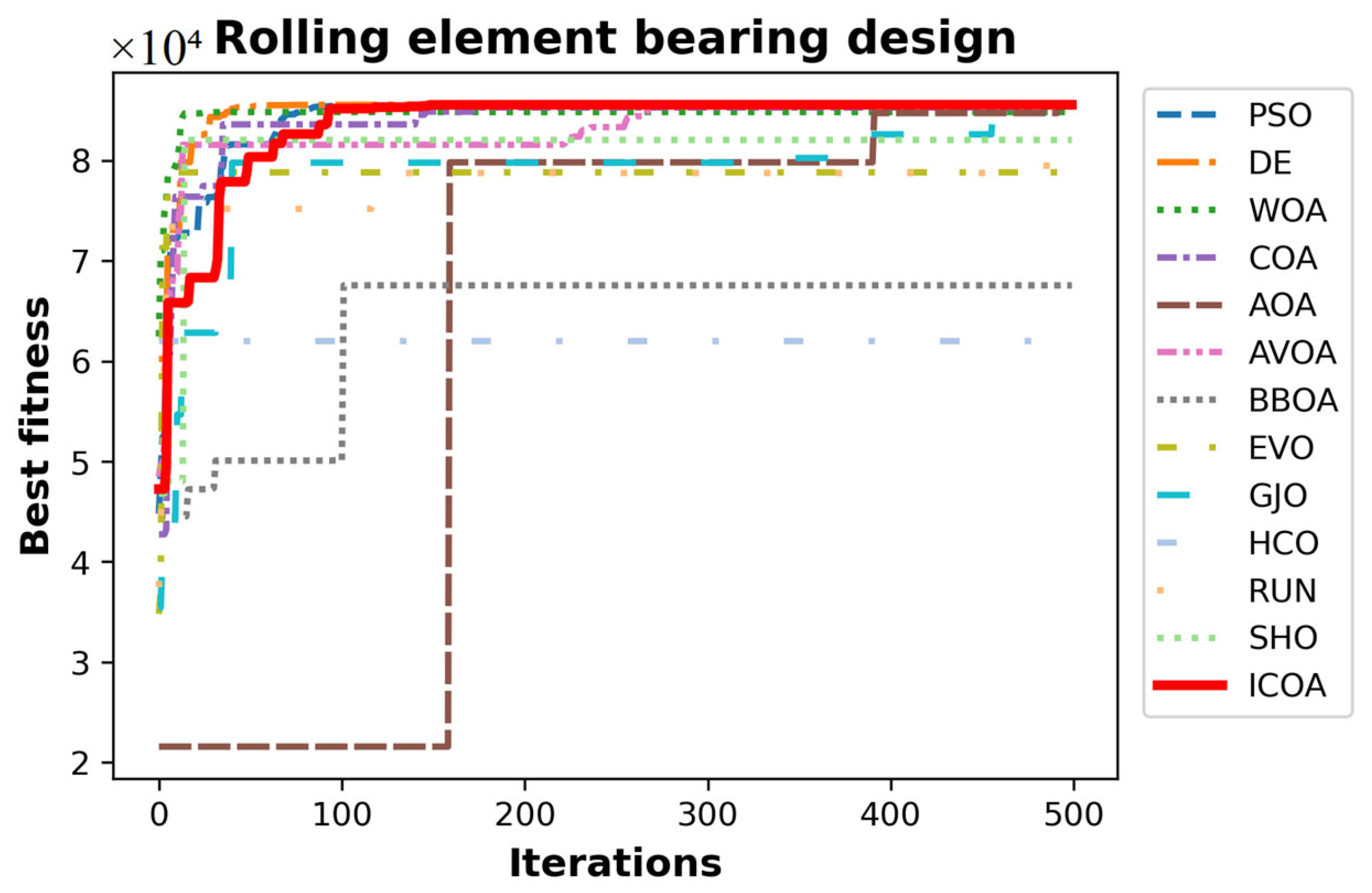
4.5.3. Rolling Element Bearing Design
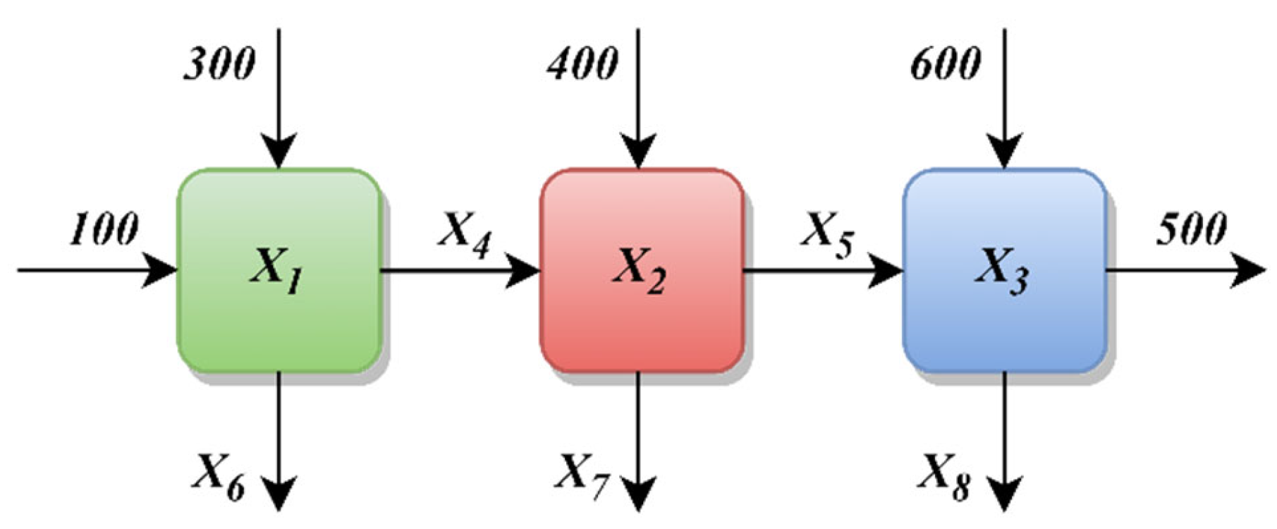
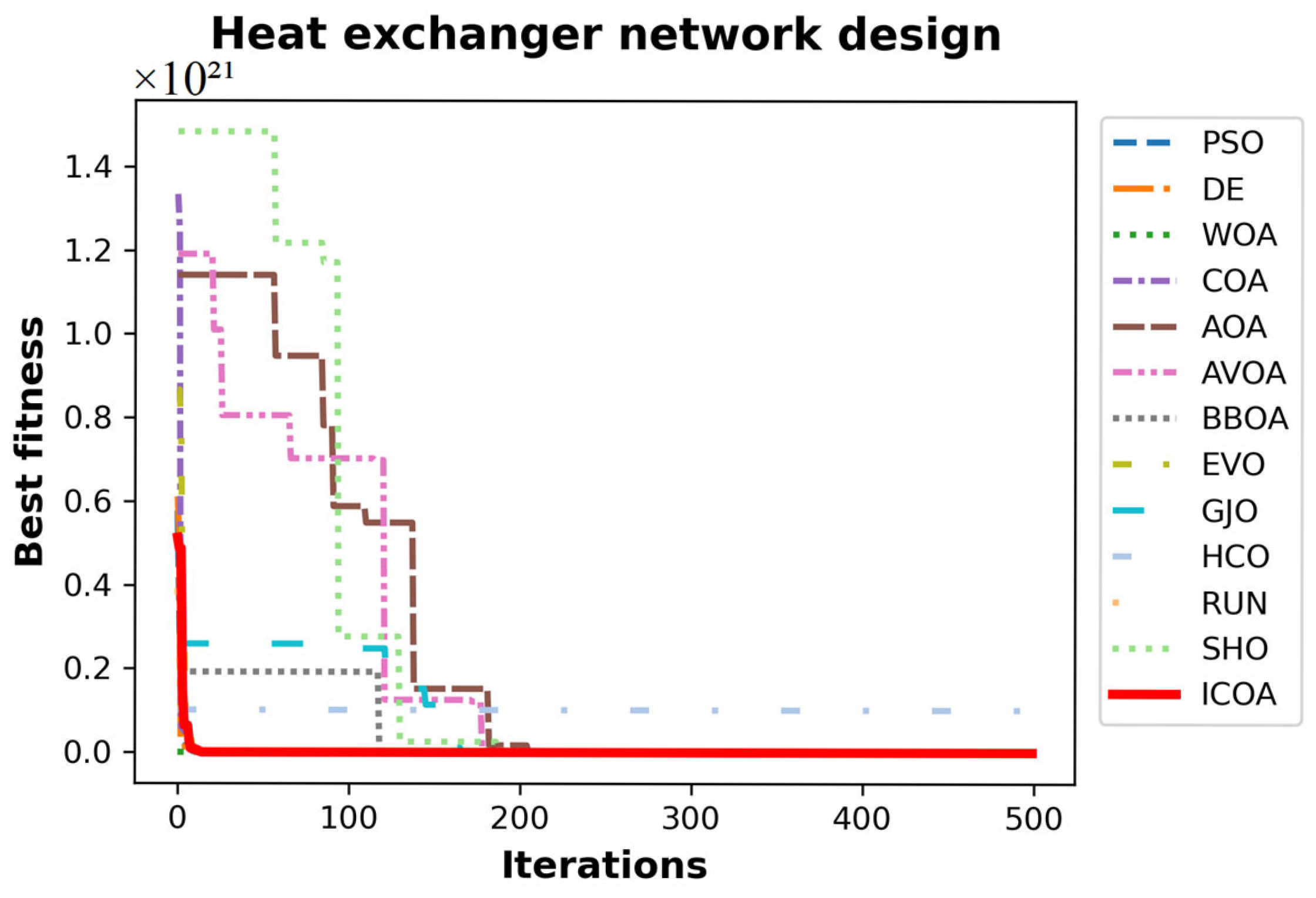
4.5.4. Heat Exchanger Network Design
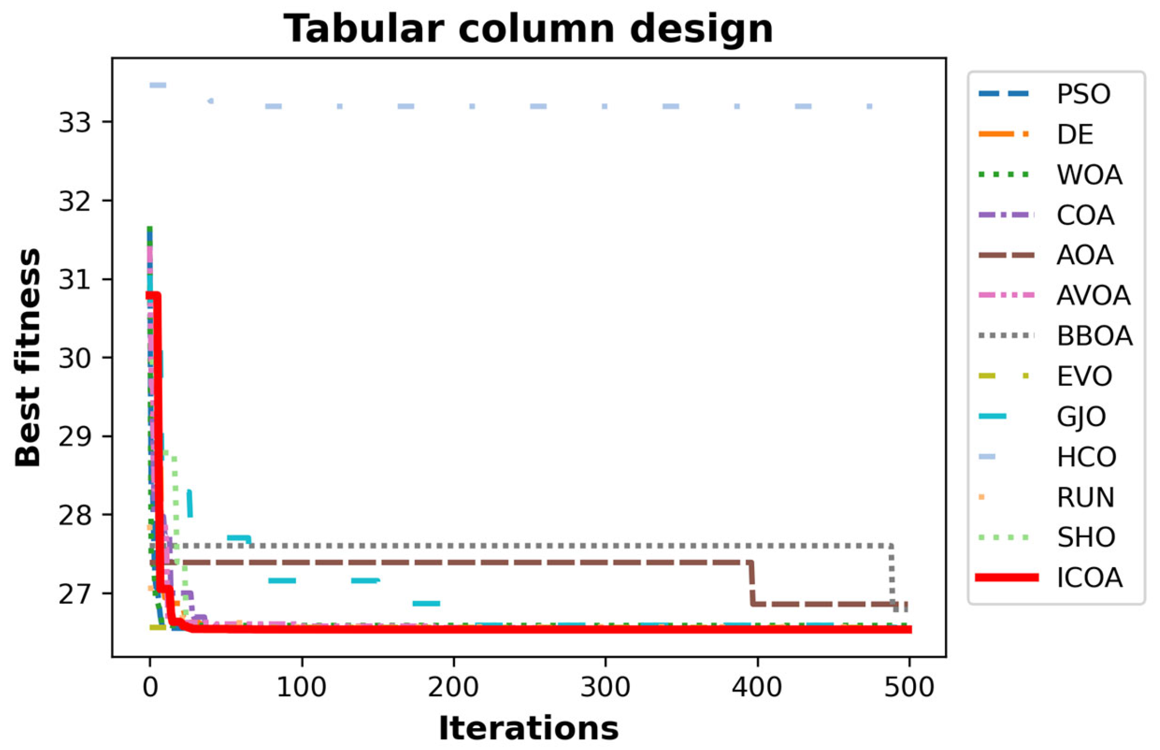
4.5.5. Tabular Column Design
4.6. Critical Assessment of ICOA Implementation
4.6.1. Algorithmic Strengths
4.6.2. Limitations and Drawbacks
4.6.3. Performance Assessment
4.6.4. Recommendations
5. ROAS Rate Problem
6. Discussion
7. Conclusions
- In the competition stage of the ICOA, step length is inversely proportional to iteration. This enables the competition stage to help exploration at low iteration numbers and exploitation at high iteration numbers.
- The randomness of the mapping vector increases the stochastic property of the ICOA.
- CEC-2014 test results indicate that the ICOA is superior to its competitor algorithms. It is a significant result that the ICOA’s efficiency does not decrease, especially when the dimension of the problem increases.
- By means of the mapping vector, in high-dimensional problems, updating only some dimensions at a time both reduces the computational load of the algorithm and controls excessive randomness.
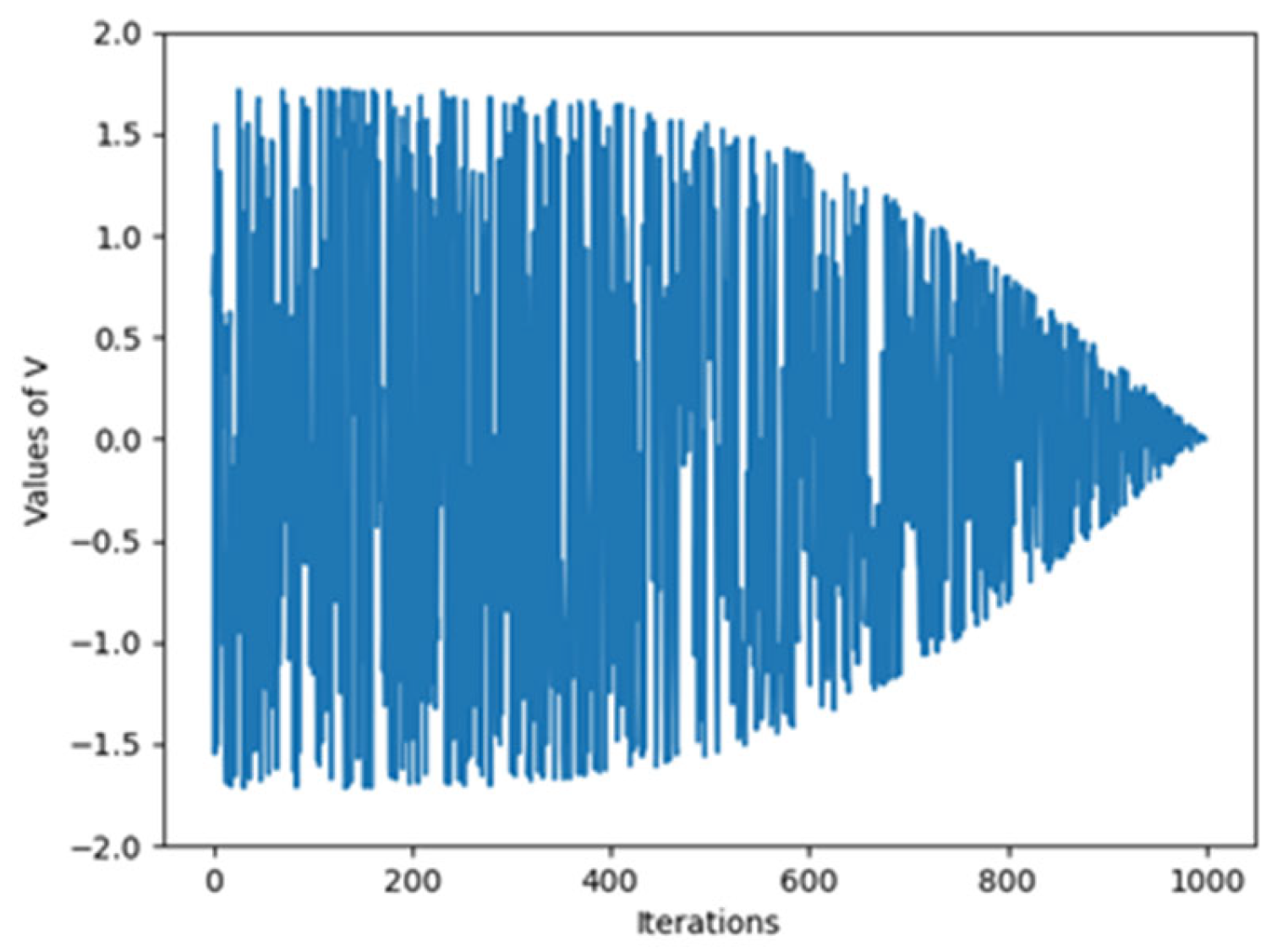
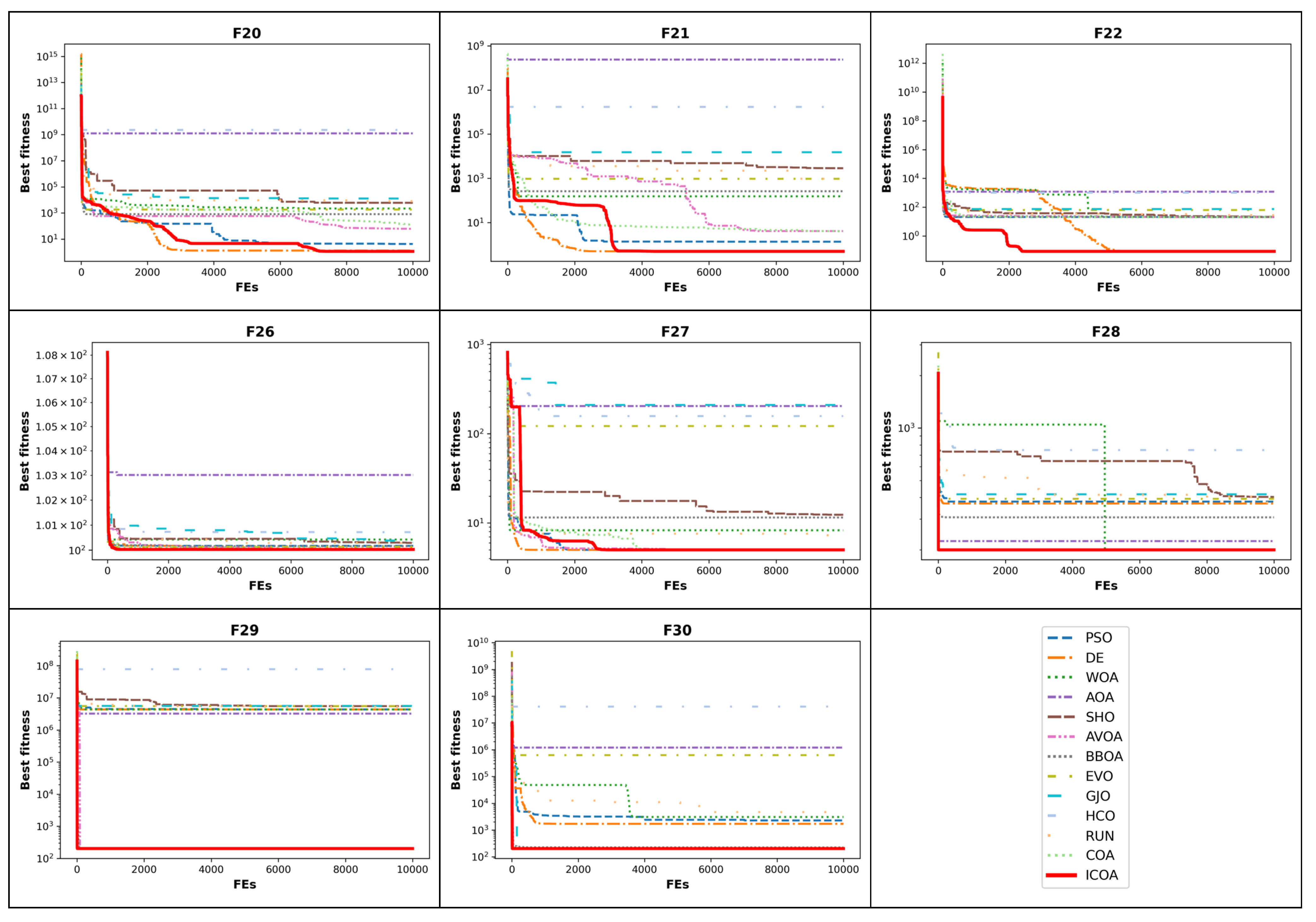
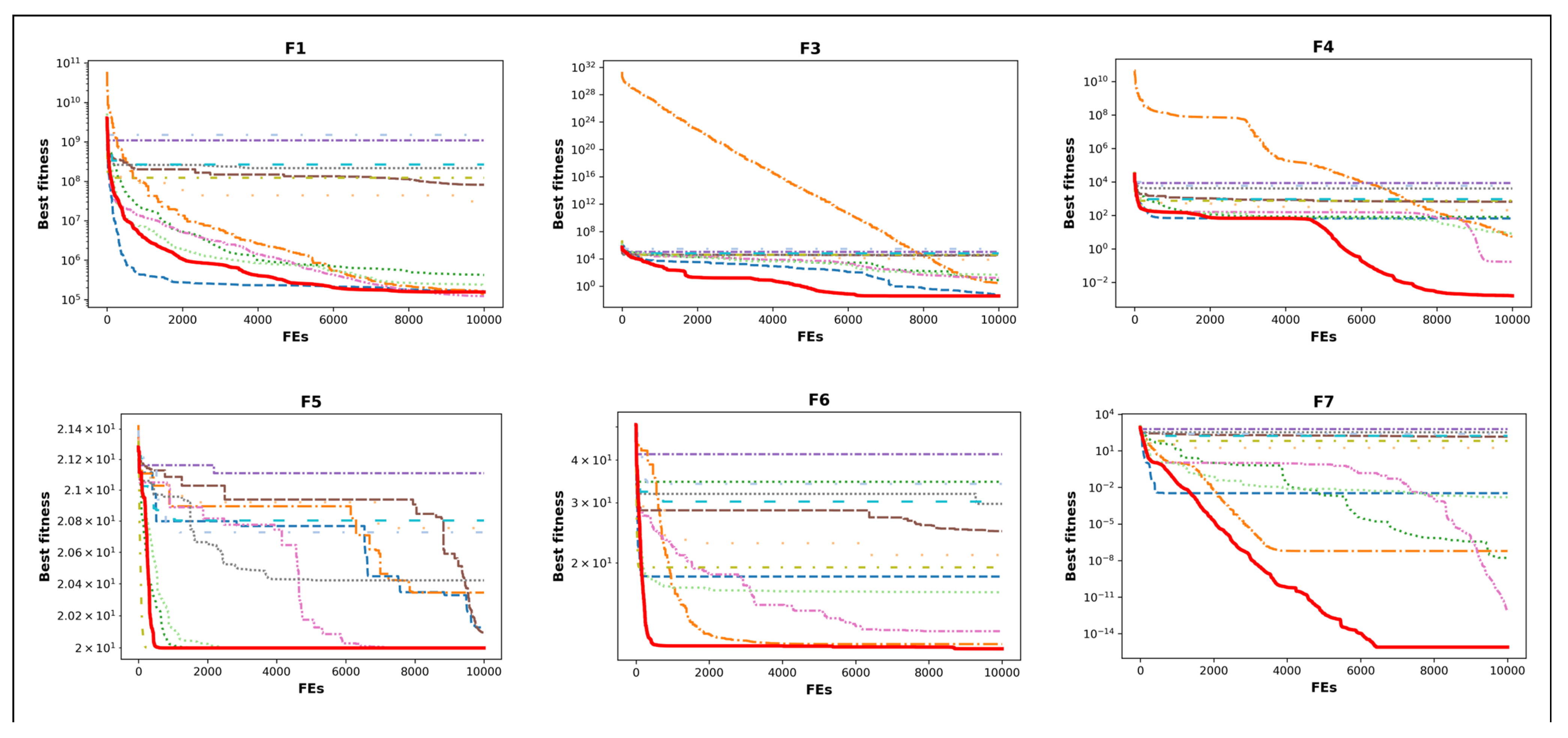
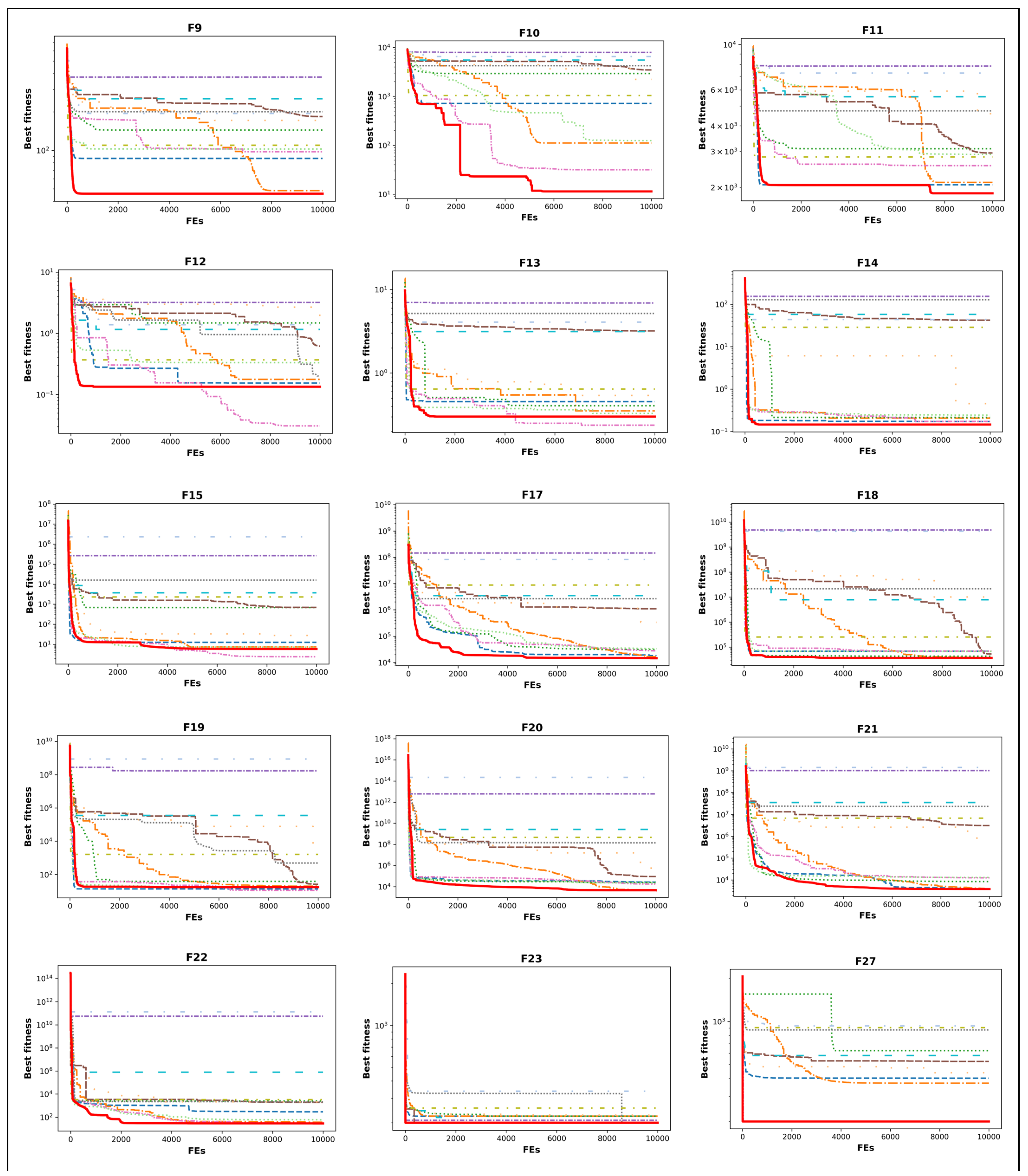
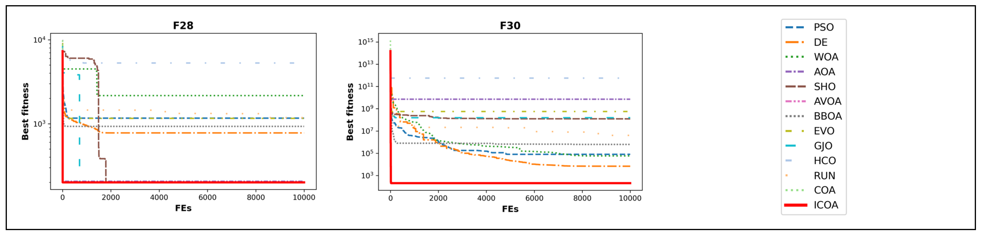
- Studying convergence curves, it is observed that the ICOA has a better curve than the COA. This verifies that the improvements made in the competition stage are successful. The number one reason why the ICOA has a better slope is that it performs exploration at low iteration numbers and exploitation at high iteration numbers. The second reason is the mapping vector of the ICOA.
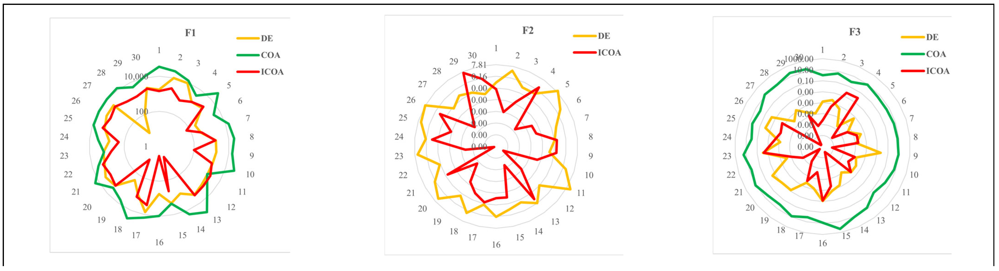
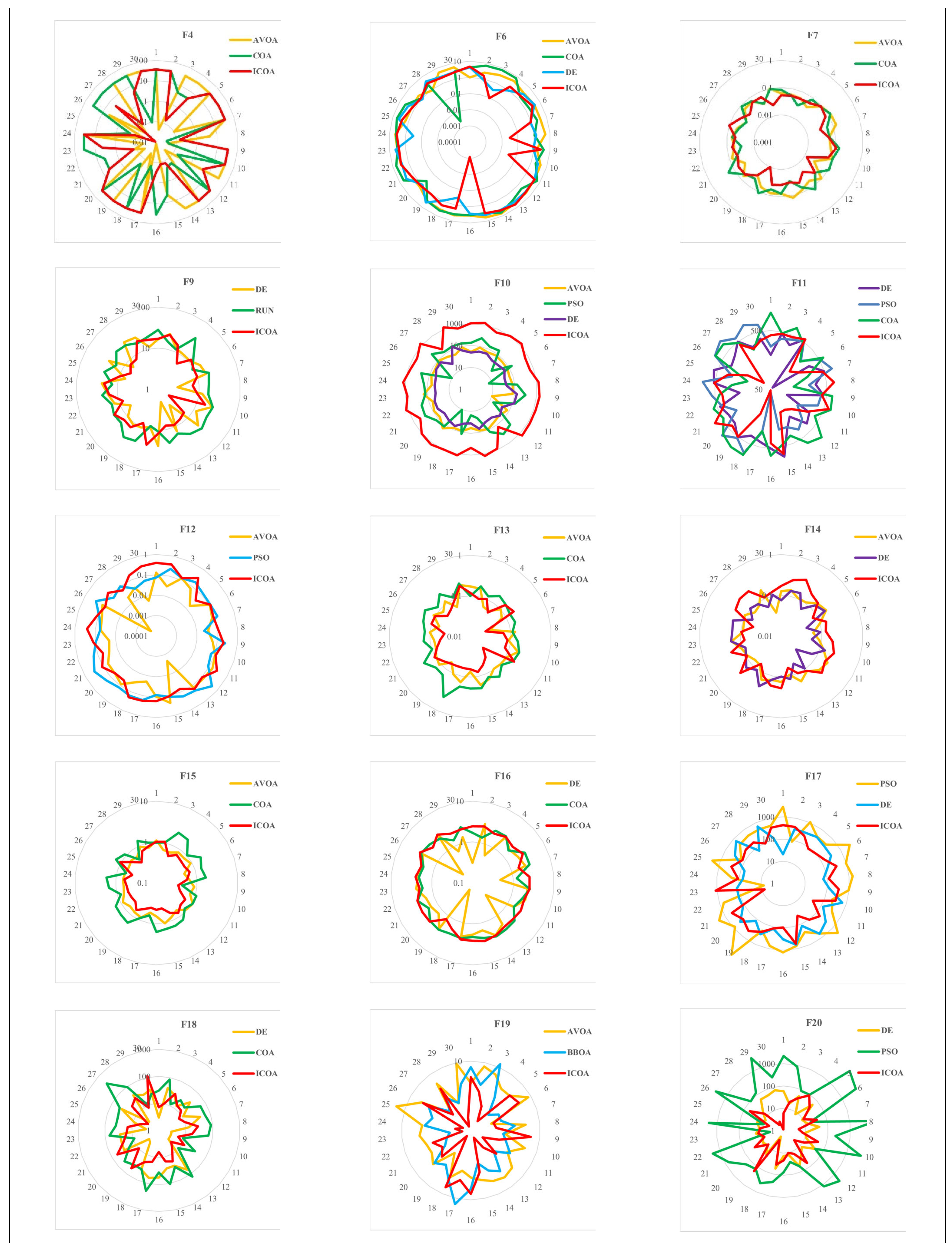
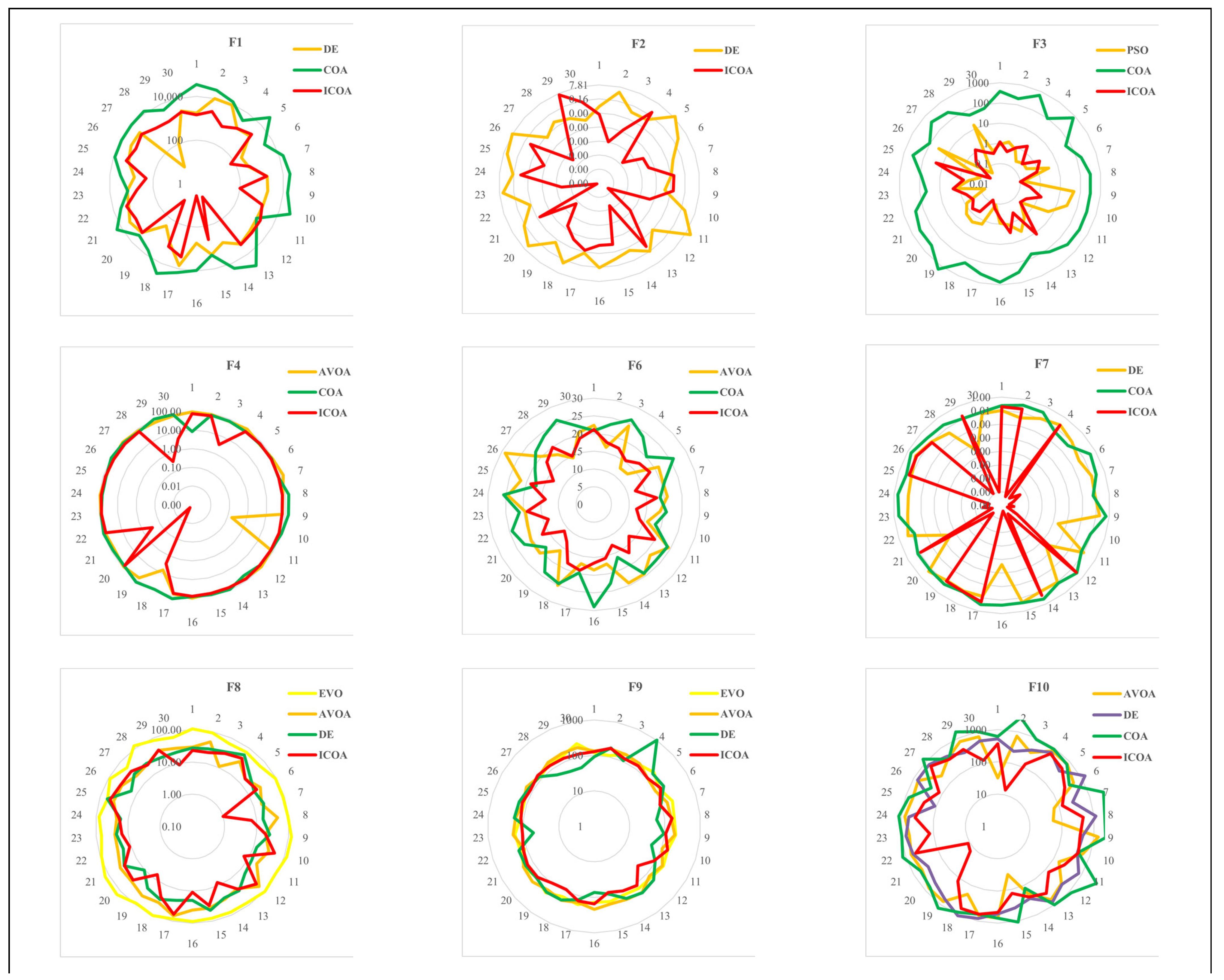
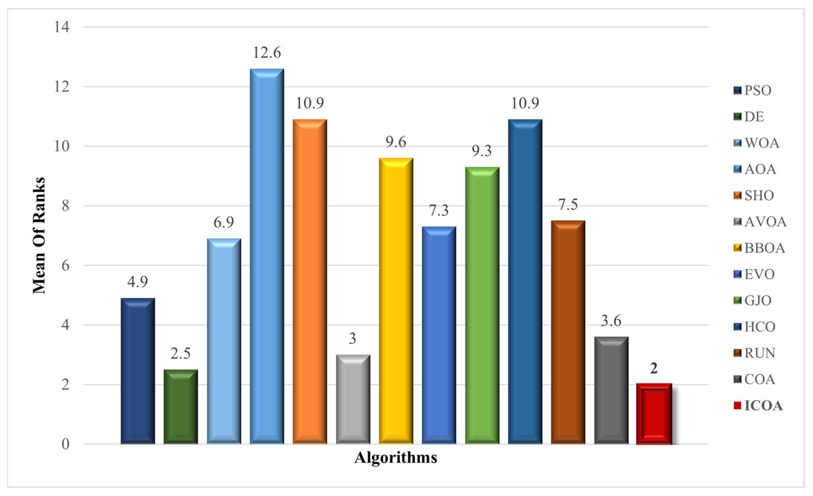
- Radar graphics indicate that the ICOA has more consistent results than its competitors.
- Scalability analysis indicates that the ICOA is the optimizer that is the least affected algorithm by the dimension increase.
- The results of engineering design problems provide the promising impression that the ICOA could solve real-world problems.
- The ICOA’s success in the ROAS problem heralds that it could solve complex real-world problems. The reason for the ICOA’s success in this problem is the improvements made in the competition stage. Removing the parameter prevents the ICOA from being caught by the local minimum trap.
Funding
Institutional Review Board Statement
Informed Consent Statement
Data Availability Statement
Conflicts of Interest
Nomenclature
| Temperature | |
| Crayfish intake | |
| , and | Control parameter |
| The best temperature for crayfish | |
| Iteration | |
| Maximum iteration | |
| Cave location | |
| Best location | |
| Best location (current population) | |
| The position of the ith agent in the jth dimension at the tth iteration | |
| The position of the ith agent in the jth dimension at the (t + 1)th iteration | |
| The position of the randomly selected zth agent from the population in the jth dimension at the tth iteration | |
| Population size | |
| Randomly selected agent | |
| food factor | |
| location of food | |
| Fitness value of agent i | |
| Fitness value of the food | |
| step length | |
| mapping vector | |
| Dimension of the problem | |
| MHA | Meta-heuristic algorithms |
| FE | Function evaluations |
| WSRT | Wilcoxon Signed-Rank Test |
| PSO | Particle Swarm Optimization |
| DE | Differential Evolution |
| WOA | Whale Optimization Algorithm |
| AOA | Arithmetic Optimization Algorithm |
| AVOA | African Vultures Optimization Algorithm |
| GJO | Golden Jackal Optimization |
| SHO | Sea-Horse Optimizer |
| EVO | Energy Valley Optimizer |
| HCO | Human Conception Optimizer |
| RUN | RUNge Kutta optimizer |
| BBOA | Brown-Bear Optimization Algorithm |
| COA | Crayfish Optimization Algorithm |
| ICOA | Improved Crayfish Optimization Algorithm |
| ROAS | Return on advertising spend |
| AS | Advertising spend |
| R | Revenue |
| APO | Artificial Protozoa Optimizer |
| FLA | Flood Algorithm |
| GGO | Greylag Goose Optimization |
| HO | Hippopotamus Optimization |
| HOA | Hiking Optimization Algorithm |
| CFOA | Catch Fish Optimization Algorithm |
| EEFO | Electric Eel Foraging Optimization |
| PO | Puma optimizer |
Appendix A

| Keywords | Advertising Spend | Num. of Impressions | Num. of Clicks | Hit Rate(%) | Sales Volume | Revenue | ROAS | Proposed CPM | Actual CPM | Selected CPM |
|---|---|---|---|---|---|---|---|---|---|---|
| Makarna lutfen | 1299.50 | 9532 | 156 | 1.64 | 130 | 18,940.01 | 14.57 | 42.51 | 136.33 | 225.42 |
| Baby biscuit | 462.85 | 8165 | 58 | 0.71 | 8 | 1277.16 | 2.76 | 18.41 | 56.69 | 206.04 |
| Biscuit | 16.56 | 4523 | 14 | 0.31 | 32 | 5251.80 | 317.14 | 15.22 | 3.66 | 145.51 |
| Organic | 116.36 | 1742 | 17 | 0.98 | 3 | 312.59 | 2.69 | 18.43 | 66.80 | 211.30 |
| Pasta | 402.09 | 6377 | 18 | 0.28 | 1 | 105.61 | 0.26 | 64.72 | 63.05 | 86.76 |
| Toddler food | 37.40 | 830 | 37 | 4.46 | 13 | 1667.82 | 44.59 | 21.00 | 45.06 | 101.03 |
| Baby semolina | 93.94 | 1180 | 33 | 2.80 | 21 | 2623.33 | 27.93 | 32.65 | 79.61 | 87.34 |
| Baby tarhana | 51.98 | 832 | 9 | 1.08 | 3 | 434.52 | 8.36 | 37.28 | 62.48 | 102.37 |
| Gluten-free pasta | 43.91 | 1207 | 9 | 0.75 | 6 | 612.40 | 13.95 | 12.37 | 36.38 | 53.18 |
| Keywords | Advertising Spend | Num. of Impressions | Num. of Clicks | Hit Rate (%) | Sales Volume | Revenue | ROAS | Proposed CPM | Actual CPM | Selected CPM |
|---|---|---|---|---|---|---|---|---|---|---|
| Makarna lutfen | 442.97 | 7497 | 83 | 1.11 | 92 | 13,709.16 | 30.95 | 73.57 | 59.09 | 124.99 |
| Baby semolina | 118.11 | 1905 | 45 | 2.36 | 9 | 1538.10 | 13.02 | 28.05 | 62.00 | 103.69 |
| Pasta | 148.75 | 3353 | 12 | 0.36 | 5 | 929.50 | 6.25 | 30.48 | 44.36 | 76.92 |
| Baby tarhana | 50.68 | 829 | 36 | 4.34 | 6 | 746.40 | 14.73 | 41.18 | 61.13 | 67.88 |
| Gluten-free pasta | 51.18 | 2177 | 51 | 2.34 | 5 | 822.50 | 16.07 | 13.30 | 23.51 | 45.05 |
| Pudding | 2.36 | 933 | 3 | 0.32 | 3 | 459.70 | 194.79 | 10.28 | 2.53 | 50.28 |
| Toddler food | 46.34 | 748 | 10 | 1.34 | 2 | 309.80 | 6.69 | 45.59 | 61.95 | 97.84 |
| Organic | 0.25 | 132 | 3 | 2.27 | 10 | 1405.63 | 5622.52 | 12.37 | 1.89 | 52.37 |
| Keywords | Advertising Spend | Num. of Impressions | Num. of Clicks | Hit Rate (%) | Sales Volume | Revenue | ROAS | Proposed CPM | Actual CPM | Selected CPM |
|---|---|---|---|---|---|---|---|---|---|---|
| Pudding | 1076.37 | 27,121 | 145 | 0.53 | 4 | 1106.6 | 1.03 | 14.46 | 39.69 | 74.4 |
| Makarna lutfen | 10,331.77 | 94,109 | 10,065 | 10.7 | 10,703 | 1,211,873.38 | 117.3 | 23.4 | 109.79 | 138 |
| Organic | 131.63 | 5060 | 87 | 1.72 | 6 | 599.19 | 4.55 | 38.69 | 26.01 | 72 |
| Pasta | 906.84 | 7287 | 31 | 0.43 | 10 | 661 | 0.73 | 28.17 | 124.45 | 145.71 |
| Baby curd | 9.86 | 242 | 9 | 3.72 | 13 | 1952.44 | 198.02 | 14.24 | 40.74 | 57 |
| Baby butter | 2.11 | 110 | 9 | 8.18 | 4 | 999.78 | 473.83 | 12.37 | 19.18 | 21 |
| Toddler food | 1449.46 | 15,005 | 252 | 1.68 | 93 | 11,648.8 | 8.04 | 40.98 | 96.6 | 541 |
| Keywords | Advertising Spend | Num. of Impressions | Num. of Clicks | Hit Rate (%) | Sales Volume | Revenue | ROAS | Proposed CPM | Actual CPM | Selected CPM |
|---|---|---|---|---|---|---|---|---|---|---|
| Makarna lutfen | 661.88 | 9722 | 83 | 0.85 | 138 | 20,105.91 | 30.38 | 63.96 | 68.08 | 74.65 |
| Toddler food | 206.31 | 2750 | 18 | 0.65 | 8 | 997.61 | 4.84 | 48.15 | 75.02 | 112.41 |
| Pasta | 404.93 | 5280 | 22 | 0.42 | 1 | 319.9 | 0.79 | 25.69 | 76.69 | 104.72 |
| Organic | 6.83 | 200 | 4 | 2 | 3 | 541.7 | 79.31 | 11.06 | 34.15 | 40.79 |
| Biscuit | 1115.59 | 13,124 | 30 | 0.23 | 8 | 1447.2 | 1.3 | 49.36 | 85 | 86.39 |
| Baby biscuit | 36.96 | 708 | 8 | 1.13 | 4 | 1134.6 | 30.7 | 38.62 | 52.2 | 102.37 |
| Baby semolina | 1566.92 | 19,175 | 509 | 2.65 | 189 | 21,785.87 | 13.9 | 25.14 | 81.72 | 163.4 |
| Keywords | Advertising Spend | Num. of Impressions | Num. of Clicks | Hit Rate (%) | Sales Volume | Revenue | ROAS | Proposed CPM | Actual CPM | Selected CPM |
|---|---|---|---|---|---|---|---|---|---|---|
| Makarna lutfen | 17,665.35 | 11,4206 | 13,709 | 12 | 13,790 | 1,811,070.41 | 102.52 | 81.57 | 154.68 | 287 |
| Pasta | 7494.32 | 56,982 | 638 | 1.12 | 371 | 53,609.57 | 7.15 | 70.41 | 131.52 | 212 |
| Toddler food | 1784.95 | 12,867 | 349 | 2.71 | 111 | 14,323.48 | 8.02 | 41.9 | 138.72 | 370 |
| Baby semolina | 5198.98 | 37,666 | 955 | 2.54 | 342 | 38,720.82 | 7.45 | 25.08 | 138.03 | 910 |
| Baby tarhana | 2780.55 | 16,440 | 381 | 2.32 | 131 | 16,951.23 | 6.1 | 27.39 | 169.13 | 291 |
| Organic | 4511.94 | 17,223 | 337 | 1.96 | 26 | 3479.74 | 0.77 | 57.02 | 261.97 | 112 |
| Baby butter | 4389.9 | 60,975 | 308 | 0.51 | 27 | 3451.92 | 0.79 | 67.66 | 72 | 170 |
| Rice flour | 107.78 | 2770 | 24 | 0.87 | 10 | 1773 | 16.45 | 16.71 | 38.91 | 93.26 |
| Keywords | Advertising Spend | Num of Impressions | Num. of Clicks | Hit Rate (%) | Sales Volume | Revenue | ROAS | Proposed CPM | Actual CPM | Selected CPM |
|---|---|---|---|---|---|---|---|---|---|---|
| Makarna lutfen | 300.51 | 6952 | 53 | 0.76 | 54 | 9519.31 | 31.68 | 54.93 | 43.23 | 65.21 |
| Rice flour | 183.78 | 6480 | 36 | 0.56 | 5 | 859.5 | 4.68 | 13.62 | 28.36 | 52.37 |
| Organic | 36.74 | 796 | 27 | 3.39 | 8 | 1515.2 | 41.24 | 12.37 | 46.16 | 61.02 |
| Pasta | 12.98 | 1311 | 12 | 0.92 | 6 | 931.4 | 71.76 | 20.57 | 9.9 | 57.29 |
| Toddler food | 3292.64 | 33,583 | 620 | 1.85 | 139 | 16,264.6 | 4.94 | 58.08 | 98.04 | 300 |
| Baby semolina | 9.83 | 253 | 36 | 14.23 | 20 | 2279 | 231.84 | 45.55 | 38.85 | 45 |
| Baby butter | 1655.21 | 79,968 | 583 | 0.73 | 28 | 5149.68 | 3.11 | 12.99 | 20.7 | 28 |
| Baby curd | 74.21 | 5589 | 60 | 1.07 | 18 | 2779.6 | 37.46 | 12.37 | 13.28 | 46 |
References
- Agushaka, J.O.; Ezugwu, A.E. Evaluation of Several Initialization Methods on Arithmetic Optimization Algorithm Performance. J. Intell. Syst. 2021, 31, 70–94. [Google Scholar] [CrossRef]
- Agushaka, J.O.; Ezugwu, A.E.; Abualigah, L. Dwarf Mongoose Optimization Algorithm. Comput. Methods Appl. Mech. Eng. 2022, 391, 114570. [Google Scholar] [CrossRef]
- Zhao, W.; Wang, L.; Zhang, Z.; Mirjalili, S.; Khodadadi, N.; Ge, Q. Quadratic Interpolation Optimization (QIO): A New Optimization Algorithm Based on Generalized Quadratic Interpolation and Its Applications to Real-World Engineering Problems. Comput. Methods Appl. Mech. Eng. 2023, 417, 116446. [Google Scholar] [CrossRef]
- Wang, L.; Cao, Q.; Zhang, Z.; Mirjalili, S.; Zhao, W. Artificial Rabbits Optimization: A New Bio-Inspired Meta-Heuristic Algorithm for Solving Engineering Optimization Problems. Eng. Appl. Artif. Intell. 2022, 114, 105082. [Google Scholar] [CrossRef]
- Abdel-Basset, M.; Mohamed, R.; Jameel, M.; Abouhawwash, M. Nutcracker Optimizer: A Novel Nature-Inspired Metaheuristic Algorithm for Global Optimization and Engineering Design Problems. Knowl. Based Syst. 2023, 262, 110248. [Google Scholar] [CrossRef]
- Ren, L.; Wang, Z.; Zhao, J.; Wu, J.; Lin, R.; Wu, J.; Fu, Y.; Tang, D. Shale Gas Load Recovery Modeling and Analysis after Hydraulic Fracturing Based on Genetic Expression Programming: A Case Study of Southern Sichuan Basin Shale. J. Nat. Gas. Sci. Eng. 2022, 107, 104778. [Google Scholar] [CrossRef]
- Hashim, F.A.; Hussain, K.; Houssein, E.H.; Mabrouk, M.S.; Al-Atabany, W. Archimedes Optimization Algorithm: A New Metaheuristic Algorithm for Solving Optimization Problems. Appl. Intell. 2021, 51, 1531–1551. [Google Scholar] [CrossRef]
- Panwar, D.; Saini, G.L.; Agarwal, P. Human Eye Vision Algorithm (HEVA): A Novel Approach for the Optimization of Combinatorial Problems. In Artificial Intelligence in Healthcare; Springer: Singapore, 2022. [Google Scholar]
- Qais, M.H.; Hasanien, H.M.; Turky, R.A.; Alghuwainem, S.; Tostado-Véliz, M.; Jurado, F. Circle Search Algorithm: A Geometry-Based Metaheuristic Optimization Algorithm. Mathematics 2022, 10, 1626. [Google Scholar] [CrossRef]
- Geem, Z.W.; Kim, J.H.; Loganathan, G.V. A New Heuristic Optimization Algorithm: Harmony Search. Simulation 2001, 76, 60–68. [Google Scholar] [CrossRef]
- Rajwar, K.; Deep, K.; Das, S. An Exhaustive Review of the Metaheuristic Algorithms for Search and Optimization: Taxonomy, Applications, and Open Challenges. Artif. Intell. Rev. 2023, 56, 13187–13257. [Google Scholar] [CrossRef]
- Zhang, W.; Zhao, J.; Liu, H.; Tu, L. Cleaner Fish Optimization Algorithm: A New Bio-Inspired Meta-Heuristic Optimization Algorithm. J. Supercomput. 2024, 80, 17338–17376. [Google Scholar] [CrossRef]
- Taheri, A.; RahimiZadeh, K.; Beheshti, A.; Baumbach, J.; Rao, R.V.; Mirjalili, S.; Gandomi, A.H. Partial Reinforcement Optimizer: An Evolutionary Optimization Algorithm. Expert. Syst. Appl. 2024, 238, 122070. [Google Scholar] [CrossRef]
- Demir, U.; Akgun, G.; Kocaoglu, S.; Okay, E.; Heydar, A.; Akdogan, E.; Yildirim, A.; Yazi, S.; Demirci, B.; Kaplanoglu, E. Comparative Design Improvement of the Growing Rod for the Scoliosis Treatment Considering the Mechanical Complications. IEEE Access 2023, 11, 40107–40120. [Google Scholar] [CrossRef]
- Huang, K.; Zhen, H.; Gong, W.; Wang, R.; Bian, W. Surrogate-Assisted Evolutionary Sampling Particle Swarm Optimization for High-Dimensional Expensive Optimization. Neural Comput. Appl. 2023, 1–17. [Google Scholar] [CrossRef]
- Deng, X.; He, D.; Qu, L. A Novel Hybrid Algorithm Based on Arithmetic Optimization Algorithm and Particle Swarm Optimization for Global Optimization Problems. J. Supercomput. 2024, 80, 8857–8897. [Google Scholar] [CrossRef]
- Wolpert, D.H.; Macready, W.G. No Free Lunch Theorems for Optimization. IEEE Trans. Evol. Comput. 1997, 1, 67–82. [Google Scholar] [CrossRef]
- Khouni, S.E.; Menacer, T. Nizar Optimization Algorithm: A Novel Metaheuristic Algorithm for Global Optimization and Engineering Applications. J. Supercomput. 2023, 80, 3229–3281. [Google Scholar] [CrossRef]
- Rajmohan, S.; Elakkiya, E.; Sreeja, S.R. Multi-Cohort Whale Optimization with Search Space Tightening for Engineering Optimization Problems. Neural Comput. Appl. 2023, 35, 8967–8986. [Google Scholar] [CrossRef]
- Duan, Y.; Liu, C.; Li, S.; Guo, X.; Yang, C. Manta Ray Foraging and Gaussian Mutation-Based Elephant Herding Optimization for Global Optimization. Eng. Comput. 2023, 39, 1085–1125. [Google Scholar] [CrossRef]
- Arora, S.; Singh, S. Butterfly Optimization Algorithm: A Novel Approach for Global Optimization. Soft Comput. 2019, 23, 715–734. [Google Scholar] [CrossRef]
- Hashim, F.A.; Houssein, E.H.; Hussain, K.; Mabrouk, M.S.; Al-Atabany, W. Honey Badger Algorithm: New Metaheuristic Algorithm for Solving Optimization Problems. Math. Comput. Simul. 2022, 192, 84–110. [Google Scholar] [CrossRef]
- Heidari, A.A.; Mirjalili, S.; Faris, H.; Aljarah, I.; Mafarja, M.; Chen, H. Harris Hawks Optimization: Algorithm and Applications. Future Gener. Comput. Syst. 2019, 97, 849–872. [Google Scholar] [CrossRef]
- Hashim, F.A.; Hussien, A.G. Snake Optimizer: A Novel Meta-Heuristic Optimization Algorithm. Knowl. Based Syst. 2022, 242, 108320. [Google Scholar] [CrossRef]
- Lu, Y.; Yu, X.; Hu, Z.; Wang, X. Convolutional Neural Network Combined with Reinforcement Learning-Based Dual-Mode Grey Wolf Optimizer to Identify Crop Diseases and Pests. Swarm Evol. Comput. 2025, 94, 101874. [Google Scholar] [CrossRef]
- Azizi, M.; Aickelin, U.A.; Khorshidi, H.; Baghalzadeh Shishehgarkhaneh, M. Energy Valley Optimizer: A Novel Metaheuristic Algorithm for Global and Engineering Optimization. Sci. Rep. 2023, 13, 226. [Google Scholar] [CrossRef]
- Prakash, T.; Singh, P.P.; Singh, V.P.; Singh, N. A Novel Brown-Bear Optimization Algorithm for Solving Economic Dispatch Problem. In Advanced Control and Optimization Paradigms for Energy System Operation and Management; River Publishers: Aalborg, Denmark, 2022; pp. 137–164. [Google Scholar]
- Xia, J.Y.; Li, S.; Huang, J.J.; Yang, Z.; Jaimoukha, I.M.; Gunduz, D. Metalearning-Based Alternating Minimization Algorithm for Nonconvex Optimization. IEEE Trans. Neural Netw. Learn. Syst. 2023, 34, 5366–5380. [Google Scholar] [CrossRef]
- Ariyanto, M.; Refat, C.M.M.; Hirao, K.; Morishima, K. Movement Optimization for a Cyborg Cockroach in a Bounded Space Incorporating Machine Learning. Cyborg Bionic Syst. 2023, 4, 0012. [Google Scholar] [CrossRef]
- Wang, H.; Yu, X.; Lu, Y. A Reinforcement Learning-Based Ranking Teaching-Learning-Based Optimization Algorithm for Parameters Estimation of Photovoltaic Models. Swarm Evol. Comput. 2025, 93, 101844. [Google Scholar] [CrossRef]
- Dehghani, M.; Trojovská, E.; Zuščák, T. A New Human-Inspired Metaheuristic Algorithm for Solving Optimization Problems Based on Mimicking Sewing Training. Sci. Rep. 2022, 12, 17387. [Google Scholar] [CrossRef]
- Braik, M.; Hammouri, A.; Atwan, J.; Al-Betar, M.A.; Awadallah, M.A. White Shark Optimizer: A Novel Bio-Inspired Meta-Heuristic Algorithm for Global Optimization Problems. Knowl. Based Syst. 2022, 243, 108457. [Google Scholar] [CrossRef]
- Seyyedabbasi, A.; Kiani, F. Sand Cat Swarm Optimization: A Nature-Inspired Algorithm to Solve Global Optimization Problems. Eng. Comput. 2023, 39, 2627–2651. [Google Scholar] [CrossRef]
- Ylldlz, B.S.; Mehta, P.; Panagant, N.; Mirjalili, S.; Yildiz, A.R. A Novel Chaotic Runge Kutta Optimization Algorithm for Solving Constrained Engineering Problems. J. Comput. Des. Eng. 2022, 9, 2452–2465. [Google Scholar] [CrossRef]
- Gezici, H.; Livatyalı, H. Chaotic Harris Hawks Optimization Algorithm. J. Comput. Des. Eng. 2022, 9, 216–245. [Google Scholar] [CrossRef]
- Mirjalili, S.; Mirjalili, S.M.; Lewis, A. Grey Wolf Optimizer. Adv. Eng. Softw. 2014, 69, 46–61. [Google Scholar] [CrossRef]
- Akl, D.T.; Saafan, M.M.; Haikal, A.Y.; El-Gendy, E.M. IHHO: An Improved Harris Hawks Optimization Algorithm for Solving Engineering Problems. Neural Comput. Appl. 2024, 36, 12185–12298. [Google Scholar] [CrossRef]
- Jia, H.; Rao, H.; Wen, C.; Mirjalili, S. Crayfish Optimization Algorithm. Artif. Intell. Rev. 2023, 56, 1919–1979. [Google Scholar] [CrossRef]
- Zhang, Y.; Liu, P.; Li, Y.; Zhang, Y.; Liu, P.; Li, Y. Implementation of an Enhanced Crayfish Optimization Algorithm. Biomimetics 2024, 9, 341. [Google Scholar] [CrossRef]
- Jia, H.; Zhou, X.; Zhang, J.; Abualigah, L.; Yildiz, A.R.; Hussien, A.G. Modified Crayfish Optimization Algorithm for Solving Multiple Engineering Application Problems. Artif. Intell. Rev. 2024, 57, 127. [Google Scholar] [CrossRef]
- Yuan, P.; Li, S.; Liao, Z. ECOA: An Enhanced Crayfish Optimization Algorithm for Real-World Engineering Problems. In Proceedings of the 2024 6th International Conference on Communications, Information System and Computer Engineering (CISCE), Guangzhou, China, 10–12 May 2024; pp. 804–809. [Google Scholar] [CrossRef]
- Zhang, J.; Diao, Y. Hierarchical Learning-Enhanced Chaotic Crayfish Optimization Algorithm: Improving Extreme Learning Machine Diagnostics in Breast Cancer. Mathematics 2024, 12, 2641. [Google Scholar] [CrossRef]
- Eberhart, R.; Kennedy, J. New Optimizer Using Particle Swarm Theory. In Proceedings of the Sixth International Symposium on Micro Machine and Human Science, Nagoya, Japan, 4–6 October 1995; pp. 39–43. [Google Scholar] [CrossRef]
- Kaelo, P.; Ali, M.M. A Numerical Study of Some Modified Differential Evolution Algorithms. Eur. J. Oper. Res. 2006, 169, 1176–1184. [Google Scholar] [CrossRef]
- Mirjalili, S.; Lewis, A. The Whale Optimization Algorithm. Adv. Eng. Softw. 2016, 95, 51–67. [Google Scholar] [CrossRef]
- Abualigah, L.; Diabat, A.; Mirjalili, S.; Abd Elaziz, M.; Gandomi, A.H. The Arithmetic Optimization Algorithm. Comput. Methods Appl. Mech. Eng. 2021, 376, 113609. [Google Scholar] [CrossRef]
- Abdollahzadeh, B.; Gharehchopogh, F.S.; Mirjalili, S. African Vultures Optimization Algorithm: A New Nature-Inspired Metaheuristic Algorithm for Global Optimization Problems. Comput. Ind. Eng. 2021, 158, 107408. [Google Scholar] [CrossRef]
- Chopra, N.; Mohsin Ansari, M. Golden Jackal Optimization: A Novel Nature-Inspired Optimizer for Engineering Applications. Expert. Syst. Appl. 2022, 198, 116924. [Google Scholar] [CrossRef]
- Zhao, S.; Zhang, T.; Ma, S.; Wang, M. Sea-Horse Optimizer: A Novel Nature-Inspired Meta-Heuristic for Global Optimization Problems. Appl. Intell. 2023, 53, 11833–11860. [Google Scholar] [CrossRef]
- Acharya, D.; Das, D.K. A Novel Human Conception Optimizer for Solving Optimization Problems. Sci. Rep. 2022, 12, 21631. [Google Scholar] [CrossRef]
- Ahmadianfar, I.; Heidari, A.A.; Gandomi, A.H.; Chu, X.; Chen, H. RUN beyond the Metaphor: An Efficient Optimization Algorithm Based on Runge Kutta Method. Expert. Syst. Appl. 2021, 181, 115079. [Google Scholar] [CrossRef]
- Derrac, J.; García, S.; Molina, D.; Herrera, F. A Practical Tutorial on the Use of Nonparametric Statistical Tests as a Methodology for Comparing Evolutionary and Swarm Intelligence Algorithms. Swarm Evol. Comput. 2011, 1, 3–18. [Google Scholar] [CrossRef]
- Rao, H.; Jia, H.; Wu, D.; Wen, C.; Li, S.; Liu, Q.; Abualigah, L. A Modified Group Teaching Optimization Algorithm for Solving Constrained Engineering Optimization Problems. Mathematics 2022, 10, 3765. [Google Scholar] [CrossRef]
- Rao, R.V.; Savsani, V.J.; Vakharia, D.P. Teaching–Learning-Based Optimization: A Novel Method for Constrained Mechanical Design Optimization Problems. Comput.-Aided Des. 2011, 43, 303–315. [Google Scholar] [CrossRef]
- Rajeswara Rao, B.; Tiwari, R. Optimum Design of Rolling Element Bearings Using Genetic Algorithms. Mech. Mach. Theory 2007, 42, 233–250. [Google Scholar] [CrossRef]
- Pant, M.; Thangaraj, R.; Singh, V.P. Optimization of Mechanical Design Problems Using Improved Differential Evolution Algorithm. Int. J. Recent. Trends Eng. 2009, 1, 21. [Google Scholar]
- Hsu, Y.L.; Liu, T.C. Developing a Fuzzy Proportional–Derivative Controller Optimization Engine for Engineering Design Optimization Problems. Eng. Optim. 2007, 39, 679–700. [Google Scholar] [CrossRef]
- Wang, X.; Snášel, V.; Mirjalili, S.; Pan, J.S.; Kong, L.; Shehadeh, H.A. Artificial Protozoa Optimizer (APO): A Novel Bio-Inspired Metaheuristic Algorithm for Engineering Optimization. Knowl. Based Syst. 2024, 295, 111737. [Google Scholar] [CrossRef]
- Ghasemi, M.; Golalipour, K.; Zare, M.; Mirjalili, S.; Trojovský, P.; Abualigah, L.; Hemmati, R. Flood Algorithm (FLA): An Efficient Inspired Meta-Heuristic for Engineering Optimization. J. Supercomput. 2024, 80, 22913–23017. [Google Scholar] [CrossRef]
- El-kenawy, E.S.M.; Khodadadi, N.; Mirjalili, S.; Abdelhamid, A.A.; Eid, M.M.; Ibrahim, A. Greylag Goose Optimization: Nature-Inspired Optimization Algorithm. Expert. Syst. Appl. 2024, 238, 122147. [Google Scholar] [CrossRef]
- Amiri, M.H.; Mehrabi Hashjin, N.; Montazeri, M.; Mirjalili, S.; Khodadadi, N. Hippopotamus Optimization Algorithm: A Novel Nature-Inspired Optimization Algorithm. Sci. Rep. 2024, 14, 5032. [Google Scholar] [CrossRef]
- Oladejo, S.O.; Ekwe, S.O.; Mirjalili, S. The Hiking Optimization Algorithm: A Novel Human-Based Metaheuristic Approach. Knowl. Based Syst. 2024, 296, 111880. [Google Scholar] [CrossRef]
- Jia, H.; Wen, Q.; Wang, Y.; Mirjalili, S. Catch Fish Optimization Algorithm: A New Human Behavior Algorithm for Solving Clustering Problems. Clust. Comput. 2024, 27, 13295–13332. [Google Scholar] [CrossRef]
- Zhao, W.; Wang, L.; Zhang, Z.; Fan, H.; Zhang, J.; Mirjalili, S.; Khodadadi, N.; Cao, Q. Electric Eel Foraging Optimization: A New Bio-Inspired Optimizer for Engineering Applications. Expert. Syst. Appl. 2024, 238, 122200. [Google Scholar] [CrossRef]
- Abdollahzadeh, B.; Khodadadi, N.; Barshandeh, S.; Trojovský, P.; Gharehchopogh, F.S.; El-kenawy, E.S.M.; Abualigah, L.; Mirjalili, S. Puma Optimizer (PO): A Novel Metaheuristic Optimization Algorithm and Its Application in Machine Learning. Clust. Comput. 2024, 27, 5235–5283. [Google Scholar] [CrossRef]


| Algorithms | Parameter Settings |
|---|---|
| PSO | |
| DE | |
| WOA | |
| AOA | |
| AVOA | |
| GJO | |
| SHO | |
| EVO | |
| HCO | |
| RUN | |
| BBOA | |
| COA | |
| ICOA |
| Func. | Index | Algorithms | ||||||||||||
|---|---|---|---|---|---|---|---|---|---|---|---|---|---|---|
| PSO | DE | WOA | AOA | SHO | AVOA | BBOA | EVO | GJO | HCO | RUN | COA | ICOA | ||
| F1 | Min | 1.34 × 101 | 8.78 × 100 | 1.34 × 101 | 4.93 × 10⁷ | 2.20 × 10⁶ | 1.66 × 10³ | 2.23 × 10⁵ | 3.45 × 10⁶ | 5.77 × 10⁶ | 9.47 × 10⁷ | 1.33 × 10⁵ | 1.46 × 10³ | 3.59 × 100 |
| Ave | 3.02 × 10³ | 2.28 × 10³ | 3.47 × 10⁶ | 3.47 × 10⁸ | 8.95 × 10⁶ | 1.51 × 10⁴ | 4.36 × 10⁶ | 2.06 × 10⁷ | 1.21 × 10⁷ | 3.27 × 10⁸ | 6.41 × 10⁵ | 1.39 × 10⁴ | 1.44 × 10³ | |
| Std | 4.15 × 10³ | 2.37 × 10³ | 1.00 × 10⁷ | 2.12 × 10⁸ | 4.40 × 10⁶ | 8.14 × 10³ | 4.96 × 10⁶ | 1.45 × 10⁷ | 3.19 × 10⁶ | 1.89 × 10⁸ | 4.80 × 10⁵ | 1.15 × 10⁴ | 9.64 × 10² | |
| F2 | Min | 5.23 × 10⁻² | 5.95 × 10⁻⁴ | 1.07 × 101 | 7.25 × 10⁹ | 5.72 × 101 | 2.24 × 101 | 1.67 × 10⁸ | 3.41 × 10⁷ | 6.51 × 10⁸ | 4.74 × 10⁹ | 2.61 × 10⁵ | 1.60 × 10⁻¹ | 1.99 × 10⁻¹¹ |
| Ave | 2.54 × 10² | 2.07 × 100 | 3.35 × 10³ | 1.04 × 10¹⁰ | 4.71 × 10⁸ | 3.27 × 10³ | 1.63 × 10⁹ | 6.61 × 10⁸ | 1.67 × 10⁹ | 1.08 × 10¹⁰ | 1.80 × 10⁷ | 1.67 × 10³ | 1.91 × 10⁻¹ | |
| Std | 7.45 × 10² | 5.85 × 100 | 3.99 × 10³ | 2.13 × 10⁹ | 5.75 × 10⁸ | 3.86 × 10³ | 1.06 × 10⁹ | 4.73 × 10⁸ | 4.19 × 10⁸ | 3.51 × 10⁹ | 1.13 × 10⁷ | 2.57 × 10³ | 9.33 × 10⁻¹ | |
| F3 | Min | 1.20 × 10⁻⁷ | 3.66 × 10⁻⁹ | 1.23 × 10² | 2.04 × 10⁴ | 1.31 × 10³ | 1.86 × 101 | 4.85 × 10² | 9.40 × 10² | 2.87 × 10³ | 5.96 × 10⁴ | 2.01 × 10² | 3.20 × 10⁻¹ | 2.66× 10⁻¹³ |
| Ave | 1.53 × 10⁻¹ | 1.09 × 10⁻³ | 9.06 × 10³ | 2.34 × 10⁶ | 4.04 × 10³ | 2.77 × 10² | 3.65 × 10³ | 1.60 × 10⁴ | 1.02 × 10⁴ | 1.56 × 10⁶ | 6.69 × 10² | 1.52 × 101 | 6.65 × 10⁻⁴ | |
| Std | 4.60 × 10⁻¹ | 2.40 × 10⁻³ | 8.86 × 10³ | 2.93 × 10⁶ | 2.23 × 10³ | 1.74 × 10² | 2.35 × 10³ | 1.79 × 10⁴ | 3.51 × 10³ | 4.77 × 10⁶ | 3.28 × 10² | 4.04 × 101 | 1.97 × 10⁻³ | |
| Func. | Index | Algorithms | ||||||||||||
|---|---|---|---|---|---|---|---|---|---|---|---|---|---|---|
| PSO | DE | WOA | AOA | SHO | AVOA | BBOA | EVO | GJO | HCO | RUN | COA | ICOA | ||
| F4 | Min | 4.76 × 10⁻² | 1.56 × 10⁻² | 1.44 × 10⁻² | 5.82 × 10² | 1.89 × 100 | 1.22 × 10⁻² | 4.98 × 101 | 2.94 × 101 | 4.29 × 101 | 2.73 × 10² | 1.11 × 100 | 3.33 × 10⁻² | 1.10 × 10⁻² |
| Ave | 2.47 × 101 | 2.93 × 101 | 2.87 × 101 | 2.18 × 10³ | 5.74 × 101 | 1.90 × 101 | 1.86 × 10² | 1.37 × 10² | 6.31 × 101 | 1.24 × 10³ | 2.26 × 101 | 1.93 × 101 | 1.83 × 101 | |
| Std | 1.71 × 101 | 1.22 × 101 | 3.29 × 101 | 1.16 × 10³ | 3.30 × 101 | 1.72 × 101 | 1.24 × 10² | 7.67 × 101 | 1.83 × 101 | 5.92 × 10² | 1.52 × 101 | 1.69 × 101 | 1.68 × 101 | |
| F5 | Min | 2.00 × 101 | 2.01 × 101 | 2.00 × 101 | 2.05 × 101 | 2.00 × 101 | 2.00 × 101 | 1.60 × 101 | 2.00 × 101 | 2.02 × 101 | 2.01 × 101 | 8.11 × 100 | 1.99 × 101 | 2.00 × 101 |
| Ave | 2.01 × 101 | 2.02 × 101 | 2.01 × 101 | 2.10 × 101 | 2.00 × 101 | 2.00 × 101 | 1.99 × 101 | 2.03 × 101 | 2.03 × 101 | 2.03 × 101 | 1.99 × 101 | 2.00 × 101 | 2.00 × 101 | |
| Std | 9.70 × 10⁻² | 5.48 × 10⁻² | 1.26 × 10⁻¹ | 1.68 × 10⁻¹ | 4.56 × 10⁻² | 3.23 × 10⁻² | 7.45 × 10⁻¹ | 3.32 × 10⁻¹ | 7.02 × 10⁻² | 1.15 × 10⁻¹ | 2.22 × 100 | 1.37 × 10⁻² | 5.31 × 10⁻³ | |
| F6 | Min | 8.86 × 10⁻¹ | 3.26 × 10⁻¹ | 6.64 × 100 | 1.00 × 101 | 3.03 × 100 | 9.03 × 10⁻¹ | 2.96 × 100 | 1.11 × 100 | 5.50 × 100 | 4.63 × 100 | 1.86 × 100 | 2.49 × 10⁻³ | 8.44 × 10⁻⁴ |
| Ave | 4.11 × 100 | 2.55 × 100 | 9.04 × 100 | 1.22 × 101 | 5.10 × 100 | 3.47 × 100 | 5.40 × 100 | 3.85 × 100 | 6.62 × 100 | 8.13 × 100 | 3.55 × 100 | 3.63 × 100 | 2.27 × 100 | |
| Std | 1.40 × 100 | 1.50 × 100 | 1.23 × 100 | 9.29 × 10⁻¹ | 1.23 × 100 | 1.53 × 100 | 1.14 × 100 | 1.62 × 100 | 8.47 × 10⁻¹ | 1.85 × 100 | 8.85 × 10⁻¹ | 2.06 × 100 | 1.50 × 100 | |
| F7 | Min | 9.11 × 10⁻² | 3.94 × 10⁻² | 1.19 × 100 | 7.65 × 101 | 1.21 × 100 | 2.46 × 10⁻² | 3.07 × 100 | 1.47 × 100 | 7.17 × 100 | 6.30 × 100 | 8.28 × 10⁻¹ | 2.84 × 10⁻² | 9.86 × 10⁻³ |
| Ave | 2.52 × 10⁻¹ | 1.50 × 10⁻¹ | 9.50 × 100 | 1.89 × 10² | 1.20 × 101 | 6.88 × 10⁻² | 3.74 × 101 | 1.25 × 101 | 1.34 × 101 | 3.56 × 101 | 1.38 × 100 | 7.44 × 10⁻² | 5.16 × 10⁻² | |
| Std | 1.81 × 10⁻¹ | 7.52 × 10⁻² | 6.08 × 100 | 4.88 × 101 | 1.34 × 101 | 2.78 × 10⁻² | 2.78 × 101 | 8.45 × 100 | 4.39 × 100 | 1.83 × 101 | 2.65 × 10⁻¹ | 3.59 × 10⁻² | 2.32 × 10⁻² | |
| F8 | Min | 5.97 × 100 | 0.00 × 100 | 9.95 × 100 | 8.54 × 101 | 1.59 × 101 | 0.00 × 100 | 1.50 × 101 | 4.38 × 100 | 3.35 × 101 | 1.81 × 101 | 2.03 × 100 | 1.29 × 10⁻⁹ | 0.00 × 100 |
| Ave | 1.85 × 101 | 2.17 × 100 | 4.07 × 101 | 1.25 × 10² | 2.56 × 101 | 1.61 × 100 | 2.72 × 101 | 1.15 × 101 | 4.06 × 101 | 3.99 × 101 | 1.21 × 101 | 5.35 × 100 | 1.16 × 100 | |
| Std | 8.27 × 100 | 1.28 × 100 | 1.77 × 101 | 1.57 × 101 | 7.59 × 100 | 9.25 × 10⁻¹ | 7.37 × 100 | 4.00 × 100 | 4.47 × 100 | 1.30 × 101 | 4.34 × 100 | 7.85 × 100 | 8.28 × 10⁻¹ | |
| F9 | Min | 1.09 × 101 | 2.08 × 100 | 1.59 × 101 | 6.99 × 101 | 2.31 × 101 | 9.95 × 100 | 1.91 × 101 | 8.78 × 100 | 3.69 × 101 | 1.81 × 101 | 8.25 × 100 | 6.98 × 100 | 1.99 × 100 |
| Ave | 2.56 × 101 | 1.39 × 101 | 5.02 × 101 | 9.37 × 101 | 3.41 × 101 | 2.36 × 101 | 2.91 × 101 | 1.93 × 101 | 4.93 × 101 | 3.52 × 101 | 1.92 × 101 | 3.16 × 101 | 1.19 × 101 | |
| Std | 8.74 × 100 | 7.06 × 100 | 1.73 × 101 | 8.99 × 100 | 7.83 × 100 | 7.86 × 100 | 5.46 × 100 | 6.33 × 100 | 3.81 × 100 | 1.46 × 101 | 6.14 × 100 | 1.64 × 101 | 5.43 × 100 | |
| F10 | Min | 7.20 × 100 | 2.72 × 101 | 3.01 × 10² | 1.09 × 10³ | 1.32 × 10² | 1.03 × 101 | 4.12 × 10² | 1.18 × 101 | 3.80 × 10² | 1.16 × 10³ | 7.23 × 100 | 2.50 × 10⁻¹ | 1.30 × 10² |
| Ave | 1.39 × 10² | 5.80 × 101 | 6.95 × 10² | 1.65 × 10³ | 4.37 × 10² | 7.82 × 101 | 7.36 × 10² | 2.23 × 10² | 7.26 × 10² | 1.64 × 10³ | 2.34 × 10² | 4.22 × 10² | 9.67 × 10² | |
| Std | 9.15 × 101 | 2.57 × 101 | 2.50 × 10² | 2.27 × 10² | 1.43 × 10² | 2.53 × 101 | 2.02 × 10² | 1.68 × 10² | 1.46 × 10² | 2.40 × 10² | 1.62 × 10² | 3.24 × 10² | 3.51 × 10² | |
| F11 | Min | 5.69 × 101 | 5.49 × 101 | 2.45 × 10² | 1.78 × 10³ | 2.70 × 10² | 1.43 × 10² | 1.15 × 10² | 2.38 × 10² | 7.16 × 10² | 9.45 × 10² | 3.34 × 10² | 1.29 × 10² | 5.22 × 101 |
| Ave | 4.53 × 10² | 3.75 × 10² | 1.13 × 10³ | 2.28 × 10³ | 6.61 × 10² | 6.40 × 10² | 7.64 × 10² | 8.08 × 10² | 1.13 × 10³ | 1.50 × 10³ | 5.99 × 10² | 5.19 × 10² | 3.61 × 10² | |
| Std | 2.16 × 10² | 1.48 × 10² | 3.48 × 10² | 2.61 × 10² | 2.04 × 10² | 2.40 × 10² | 2.72 × 10² | 2.34 × 10² | 1.59 × 10² | 2.80 × 10² | 1.64 × 10² | 2.20 × 10² | 1.85 × 10² | |
| F12 | Min | 2.29 × 10⁻² | 4.32 × 10⁻² | 3.91 × 10⁻¹ | 1.88 × 100 | 5.16 × 10⁻² | 2.26 × 10⁻⁴ | 1.15 × 10⁻¹ | 7.44 × 10⁻² | 4.15 × 10⁻¹ | 6.89 × 10⁻¹ | 3.42 × 10⁻¹ | 4.92 × 10⁻² | 4.01 × 10⁻² |
| Ave | 1.43 × 10⁻¹ | 2.17 × 10⁻¹ | 8.38 × 10⁻¹ | 4.04 × 100 | 2.36 × 10⁻¹ | 6.93 × 10⁻² | 4.06 × 10⁻¹ | 3.34 × 10⁻¹ | 7.39 × 10⁻¹ | 1.45 × 100 | 8.19 × 10⁻¹ | 3.05 × 10⁻¹ | 1.55 × 10⁻¹ | |
| Std | 9.34 × 10⁻² | 1.33 × 10⁻¹ | 2.47 × 10⁻¹ | 1.16 × 100 | 1.35 × 10⁻¹ | 5.31 × 10⁻² | 1.57 × 10⁻¹ | 1.92 × 10⁻¹ | 1.95 × 10⁻¹ | 4.31 × 10⁻¹ | 2.00 × 10⁻¹ | 1.83 × 10⁻¹ | 9.60 × 10⁻² | |
| F13 | Min | 1.72 × 10⁻¹ | 4.15 × 10⁻² | 2.73 × 10⁻¹ | 2.07 × 100 | 3.77 × 10⁻¹ | 3.26 × 10⁻² | 3.26 × 10⁻¹ | 2.30 × 10⁻¹ | 3.96 × 10⁻¹ | 1.64 × 10⁻¹ | 1.31 × 10⁻¹ | 9.67 × 10⁻² | 2.49 × 10⁻² |
| Ave | 4.61 × 10⁻¹ | 1.55 × 10⁻¹ | 6.59 × 10⁻¹ | 4.83 × 100 | 7.33 × 10⁻¹ | 1.05 × 10⁻¹ | 1.41 × 100 | 4.39 × 10⁻¹ | 7.01 × 10⁻¹ | 1.19 × 100 | 2.64 × 10⁻¹ | 1.62 × 10⁻¹ | 8.43 × 10⁻² | |
| Std | 2.09 × 10⁻¹ | 6.28 × 10⁻² | 2.37 × 10⁻¹ | 1.07 × 100 | 3.98 × 10⁻¹ | 4.01 × 10⁻² | 9.51 × 10⁻¹ | 1.34 × 10⁻¹ | 1.10 × 10⁻¹ | 8.64 × 10⁻¹ | 7.27 × 10⁻² | 5.97 × 10⁻² | 4.10 × 10⁻² | |
| F14 | Min | 4.02 × 10⁻² | 3.12 × 10⁻² | 1.04 × 10⁻¹ | 2.47 × 101 | 2.26 × 10⁻¹ | 3.90 × 10⁻² | 1.04 × 100 | 2.38 × 10⁻¹ | 9.88 × 10⁻¹ | 3.04 × 10⁻¹ | 8.05 × 10⁻² | 6.85 × 10⁻² | 5.30 × 10⁻² |
| Ave | 2.20 × 10⁻¹ | 1.08 × 10⁻¹ | 4.58 × 10⁻¹ | 3.98 × 101 | 1.54 × 100 | 1.17 × 10⁻¹ | 1.06 × 101 | 2.55 × 100 | 3.14 × 100 | 7.90 × 100 | 1.76 × 10⁻¹ | 2.01 × 10⁻¹ | 1.56 × 10⁻¹ | |
| Std | 1.59 × 10⁻¹ | 4.43 × 10⁻² | 3.64 × 10⁻¹ | 7.46 × 100 | 2.41 × 100 | 4.03 × 10⁻² | 7.33 × 100 | 2.18 × 100 | 9.37 × 10⁻¹ | 4.33 × 100 | 4.36 × 10⁻² | 8.29 × 10⁻² | 6.57 × 10⁻² | |
| F15 | Min | 7.14 × 10⁻¹ | 5.68 × 10⁻¹ | 3.24 × 100 | 1.14 × 10³ | 1.78 × 100 | 5.19 × 10⁻¹ | 2.77 × 100 | 2.68 × 100 | 6.49 × 100 | 1.13 × 10⁴ | 1.84 × 100 | 4.30 × 10⁻¹ | 3.44 × 10⁻¹ |
| Ave | 2.33 × 100 | 1.45 × 100 | 5.89 × 101 | 1.55 × 10⁴ | 4.49 × 100 | 7.64 × 10⁻¹ | 4.74 × 101 | 9.06 × 101 | 1.22 × 101 | 1.35 × 10⁵ | 2.98 × 100 | 1.24 × 100 | 6.17 × 10⁻¹ | |
| Std | 1.33 × 100 | 5.40 × 10⁻¹ | 7.12 × 101 | 1.65 × 10⁴ | 3.33 × 100 | 1.51 × 10⁻¹ | 1.37 × 10² | 2.77 × 10² | 7.99 × 100 | 1.29 × 10⁵ | 5.83 × 10⁻¹ | 4.35 × 10⁻¹ | 1.89 × 10⁻¹ | |
| F16 | Min | 1.35 × 100 | 1.52 × 10⁻¹ | 2.63 × 100 | 3.89 × 100 | 2.20 × 100 | 1.80 × 100 | 2.26 × 100 | 2.57 × 100 | 3.44 × 100 | 2.38 × 100 | 1.77 × 100 | 1.24 × 100 | 1.24 × 100 |
| Ave | 2.41 × 100 | 1.66 × 100 | 3.45 × 100 | 4.31 × 100 | 2.93 × 100 | 2.47 × 100 | 2.88 × 100 | 3.38 × 100 | 3.65 × 100 | 3.39 × 100 | 2.47 × 100 | 2.20 × 100 | 2.32 × 100 | |
| Std | 4.00 × 10⁻¹ | 8.31 × 10⁻¹ | 3.41 × 10⁻¹ | 1.81 × 10⁻¹ | 3.18 × 10⁻¹ | 3.01 × 10⁻¹ | 2.85 × 10⁻¹ | 4.04 × 10⁻¹ | 1.02 × 10⁻¹ | 4.52 × 10⁻¹ | 3.52 × 10⁻¹ | 5.01 × 10⁻¹ | 3.92 × 10⁻¹ | |
| Func. | Index | Algorithms | ||||||||||||
|---|---|---|---|---|---|---|---|---|---|---|---|---|---|---|
| PSO | DE | WOA | AOA | SHO | AVOA | BBOA | EVO | GJO | HCO | RUN | COA | ICOA | ||
| F17 | Min | 7.58 × 100 | 2.08 × 101 | 6.77 × 10² | 5.83 × 10⁵ | 4.62 × 10³ | 8.60 × 10² | 6.22 × 10² | 6.34 × 10³ | 8.93 × 10³ | 6.20 × 10⁵ | 1.60 × 10³ | 2.29 × 10² | 7.40 × 100 |
| Ave | 1.15 × 10³ | 2.73 × 10² | 1.95 × 10³ | 7.14 × 10⁶ | 9.24 × 10³ | 2.62 × 10³ | 2.74 × 10³ | 1.39 × 10⁵ | 4.33 × 10⁴ | 1.05 × 10⁷ | 8.92 × 10³ | 4.89 × 10³ | 2.51 × 10² | |
| Std | 1.68 × 10³ | 2.07 × 10² | 1.21 × 10³ | 1.03 × 10⁷ | 4.33 × 10³ | 1.42 × 10³ | 2.56 × 10³ | 4.26 × 10⁵ | 3.09 × 10⁴ | 8.43 × 10⁶ | 4.51 × 10³ | 5.48 × 10³ | 2.20 × 10² | |
| F18 | Min | 4.95 × 100 | 2.95 × 100 | 1.32 × 10² | 1.33 × 10⁶ | 1.03 × 10⁴ | 1.35 × 101 | 1.13 × 10³ | 6.16 × 10³ | 1.78 × 10⁴ | 3.90 × 10⁶ | 1.32 × 10³ | 8.46 × 100 | 2.91 × 100 |
| Ave | 4.62 × 101 | 2.39 × 101 | 5.22 × 10³ | 1.48 × 10⁸ | 1.62 × 10⁴ | 1.06 × 10³ | 9.66 × 10³ | 1.99 × 10⁶ | 1.94 × 10⁴ | 1.20 × 10⁸ | 4.11 × 10³ | 6.23 × 101 | 1.99 × 101 | |
| Std | 1.45 × 10² | 1.86 × 101 | 4.31 × 10³ | 1.61 × 10⁸ | 2.97 × 10³ | 1.18 × 10³ | 4.91 × 10³ | 6.97 × 10⁶ | 4.36 × 10² | 1.08 × 10⁸ | 2.38 × 10³ | 7.53 × 101 | 2.19 × 101 | |
| F19 | Min | 1.66 × 100 | 3.18 × 100 | 6.80 × 100 | 1.22 × 10⁴ | 4.32 × 100 | 2.05 × 100 | 2.02 × 100 | 5.92 × 100 | 7.99 × 100 | 1.44 × 10⁵ | 4.23 × 100 | 1.58 × 100 | 1.16 × 100 |
| Ave | 1.08 × 101 | 5.17 × 100 | 3.07 × 101 | 7.63 × 10⁶ | 8.31 × 100 | 5.72 × 100 | 4.51 × 100 | 3.80 × 10⁴ | 2.98 × 101 | 3.29 × 10⁶ | 9.35 × 100 | 7.12 × 100 | 3.55 × 100 | |
| Std | 7.61 × 100 | 1.10 × 100 | 3.93 × 101 | 1.41 × 10⁷ | 1.66 × 100 | 2.39 × 100 | 2.42 × 100 | 1.77 × 10⁵ | 9.25 × 101 | 3.33 × 10⁶ | 2.61 × 100 | 4.86 × 100 | 2.20 × 100 | |
| F20 | Min | 4.20 × 100 | 1.96 × 100 | 2.18 × 10³ | 1.26 × 10⁹ | 5.94 × 10³ | 6.04 × 101 | 8.07 × 10² | 1.81 × 10³ | 1.24 × 10⁴ | 2.30 × 10⁹ | 7.94 × 10³ | 1.30 × 10² | 1.13 × 100 |
| Ave | 1.82 × 10³ | 2.63 × 101 | 1.18 × 10⁴ | 2.34 × 10¹³ | 1.62 × 10⁴ | 5.80 × 10³ | 2.30 × 10⁴ | 4.38 × 101⁰ | 4.50 × 10⁴ | 4.27 × 10¹² | 2.35 × 10⁴ | 6.95 × 10³ | 2.61 × 101 | |
| Std | 3.21 × 10³ | 2.03 × 101 | 1.10 × 10⁴ | 6.72 × 10¹³ | 6.85 × 10³ | 5.21 × 10³ | 2.08 × 10⁴ | 2.27 × 10¹¹ | 1.30 × 10⁵ | 9.67 × 10¹² | 1.18 × 10⁴ | 9.02 × 10³ | 3.48 × 101 | |
| F21 | Min | 1.36 × 100 | 4.98 × 10⁻¹ | 3.68 × 100 | 7.10 × 10⁵ | 2.87 × 10³ | 4.12 × 100 | 2.61 × 10² | 9.54 × 10² | 1.52 × 10⁴ | 1.72 × 10⁶ | 9.62 × 10² | 4.01 × 100 | 4.97 × 10⁻¹ |
| Ave | 4.32 × 101 | 4.09 × 100 | 5.21 × 10² | 5.18 × 10⁷ | 5.86 × 10³ | 2.18 × 10² | 2.44 × 10³ | 3.11 × 10⁵ | 1.43 × 10⁵ | 3.96 × 10⁷ | 2.50 × 10³ | 5.56 × 101 | 3.91 × 100 | |
| Std | 4.41 × 101 | 3.79 × 100 | 8.02 × 10² | 5.72 × 10⁷ | 1.18 × 10³ | 1.94 × 10² | 2.54 × 10³ | 5.71 × 10⁵ | 1.39 × 10⁵ | 3.23 × 10⁷ | 1.26 × 10³ | 5.47 × 101 | 8.48 × 100 | |
| F22 | Min | 2.06 × 101 | 8.56 × 10⁻² | 2.07 × 101 | 1.19 × 10³ | 2.13 × 101 | 2.03 × 101 | 2.10 × 101 | 6.34 × 101 | 7.39 × 101 | 1.01 × 10³ | 2.83 × 101 | 2.03 × 101 | 8.54 × 10⁻² |
| Ave | 1.83 × 10² | 5.29 × 10² | 1.20 × 10² | 3.61 × 10¹¹ | 2.06 × 10² | 7.88 × 101 | 1.19 × 10² | 3.35 × 10⁷ | 3.20 × 10² | 8.66 × 101⁰ | 4.31 × 101 | 1.35 × 10² | 9.83 × 101 | |
| Std | 9.83 × 101 | 8.17 × 10² | 1.14 × 10² | 1.34 × 10¹² | 2.56 × 10² | 9.76 × 101 | 1.34 × 10² | 1.79 × 10⁸ | 2.95 × 10² | 2.29 × 10¹¹ | 4.05 × 101 | 1.69 × 10² | 1.07 × 10² | |
| Func. | İndex | Algorithms | ||||||||||||
|---|---|---|---|---|---|---|---|---|---|---|---|---|---|---|
| PSO | DE | WOA | AOA | SHO | AVOA | BBOA | EVO | GJO | HCO | RUN | COA | ICOA | ||
| F23 | Min | 2.37 × 10² | 2.37 × 10² | 2.00 × 10² | 2.00 × 10² | 2.00 × 10² | 2.00 × 10² | 2.00 × 10² | 2.43 × 10² | 2.00 × 10² | 2.52 × 10² | 2.00 × 10² | 2.00 × 10² | 2.00 × 10² |
| Ave | 2.42 × 10² | 2.37 × 10² | 2.38 × 10² | 2.05 × 10² | 2.00 × 10² | 2.00 × 10² | 2.00 × 10² | 2.52 × 10² | 2.00 × 10² | 2.73 × 10² | 2.04 × 10² | 2.00 × 10² | 2.00 × 10² | |
| Std | 1.65 × 100 | 1.65 × 100 | 1.29 × 101 | 1.12 × 100 | 0.00 × 100 | 0.00 × 100 | 0.00 × 100 | 5.66 × 100 | 0.00 × 100 | 1.90 × 101 | 1.13 × 101 | 0.00 × 100 | 0.00 × 100 | |
| F24 | Min | 1.16 × 10² | 1.11 × 10² | 1.23 × 10² | 1.88 × 10² | 1.16 × 10² | 1.15 × 10² | 1.29 × 10² | 1.21 × 10² | 1.50 × 10² | 1.23 × 10² | 1.15 × 10² | 1.16 × 10² | 1.10 × 10² |
| Ave | 1.35 × 10² | 1.25 × 10² | 1.68 × 10² | 2.00 × 10² | 1.45 × 10² | 1.32 × 10² | 1.63 × 10² | 1.57 × 10² | 1.56 × 10² | 1.63 × 10² | 1.25 × 10² | 1.98 × 10² | 1.21 × 10² | |
| Std | 1.18 × 101 | 5.39 × 100 | 3.01 × 101 | 2.73 × 100 | 2.67 × 101 | 1.60 × 101 | 2.53 × 101 | 2.33 × 101 | 3.99 × 100 | 2.47 × 101 | 6.09 × 100 | 1.54 × 101 | 6.75 × 100 | |
| F25 | Min | 1.55 × 10² | 2.00 × 10² | 1.66 × 10² | 2.00 × 10² | 1.60 × 10² | 2.00 × 10² | 1.82 × 10² | 2.02 × 10² | 2.00 × 10² | 2.01 × 10² | 1.55 × 10² | 2.00 × 10² | 2.00 × 10² |
| Ave | 1.95 × 10² | 2.00 × 10² | 1.99 × 10² | 2.00 × 10² | 1.97 × 10² | 2.00 × 10² | 1.99 × 10² | 2.04 × 10² | 2.00 × 10² | 2.06 × 10² | 1.95 × 10² | 2.00 × 10² | 2.00 × 10² | |
| Std | 1.42 × 101 | 1.45 × 10⁻¹³ | 7.34 × 100 | 3.58 × 10⁻² | 9.47 × 100 | 0.00 × 100 | 4.35 × 100 | 1.65 × 100 | 0.00 × 100 | 1.71 × 100 | 1.49 × 101 | 0.00 × 100 | 0.00 × 100 | |
| F26 | Min | 1.00 × 10² | 1.00 × 10² | 1.00 × 10² | 1.03 × 10² | 1.00 × 10² | 1.00 × 10² | 1.00 × 10² | 1.00 × 10² | 1.00 × 10² | 1.01 × 10² | 1.00 × 10² | 1.00 × 10² | 1.00 × 10² |
| Ave | 1.00 × 10² | 1.00 × 10² | 1.01 × 10² | 1.06 × 10² | 1.04 × 10² | 1.00 × 10² | 1.01 × 10² | 1.01 × 10² | 1.01 × 10² | 1.03 × 10² | 1.00 × 10² | 1.00 × 10² | 1.00 × 10² | |
| Std | 2.14 × 10⁻¹ | 5.78 × 10⁻² | 1.99 × 10⁻¹ | 4.16 × 100 | 1.81 × 101 | 2.44 × 10⁻² | 7.24 × 10⁻¹ | 5.85 × 10⁻¹ | 3.59 × 10⁻¹ | 1.32 × 100 | 5.89 × 10⁻² | 1.53 × 10⁻¹ | 2.57 × 10⁻² | |
| F27 | Min | 5.00 × 100 | 5.00 × 100 | 8.29 × 100 | 2.04 × 10² | 1.24 × 101 | 5.00 × 100 | 1.15 × 101 | 1.22 × 10² | 2.10 × 10² | 1.58 × 10² | 7.29 × 100 | 5.00 × 100 | 5.00 × 100 |
| Ave | 3.17 × 10² | 3.37 × 10² | 3.90 × 10² | 2.04 × 10² | 3.30 × 10² | 1.48 × 10² | 3.58 × 10² | 4.14 × 10² | 3.96 × 10² | 4.25 × 10² | 3.58 × 10² | 1.83 × 10² | 6.43 × 101 | |
| Std | 1.59 × 10² | 1.36 × 10² | 7.22 × 101 | 2.89 × 10⁻¹⁴ | 1.53 × 10² | 8.77 × 101 | 1.54 × 10² | 8.54 × 101 | 1.06 × 10² | 7.71 × 101 | 1.21 × 10² | 5.35 × 101 | 9.04 × 101 | |
| F28 | Min | 3.78 × 10² | 3.69 × 10² | 2.00 × 10² | 2.24 × 10² | 4.02 × 10² | 2.00 × 10² | 3.07 × 10² | 3.92 × 10² | 4.17 × 10² | 7.47 × 10² | 3.73 × 10² | 2.00 × 10² | 2.00 × 10² |
| Ave | 5.09 × 10² | 3.83 × 10² | 7.27 × 10² | 2.24 × 10² | 5.16 × 10² | 2.00 × 10² | 3.36 × 10² | 6.00 × 10² | 5.03 × 10² | 1.10 × 10³ | 4.67 × 10² | 2.00 × 10² | 2.00 × 10² | |
| Std | 9.32 × 101 | 2.68 × 101 | 1.79 × 10² | 5.78 × 10⁻¹⁴ | 7.79 × 101 | 0.00 × 100 | 3.06 × 101 | 1.71 × 10² | 7.55 × 101 | 2.18 × 10² | 8.15 × 101 | 0.00 × 100 | 0.00 × 100 | |
| F29 | Min | 4.36 × 10⁶ | 4.36 × 10⁶ | 4.36 × 10⁶ | 3.23 × 10⁶ | 5.51 × 10⁶ | 2.02 × 10² | 2.07 × 10² | 5.54 × 10⁶ | 5.61 × 10⁶ | 7.79 × 10⁷ | 4.58 × 10⁶ | 2.02 × 10² | 2.02 × 10² |
| Ave | 4.92 × 10⁶ | 4.60 × 10⁶ | 1.21 × 10⁷ | 1.16 × 10⁷ | 8.80 × 10⁶ | 2.02 × 10² | 2.83 × 10² | 1.89 × 10⁷ | 6.88 × 10⁶ | 1.83 × 10⁸ | 5.83 × 10⁶ | 2.02 × 10² | 2.02 × 10² | |
| Std | 4.60 × 10⁵ | 3.93 × 10⁵ | 7.93 × 10⁶ | 1.92 × 10⁶ | 3.51 × 10⁶ | 0.00 × 100 | 8.13 × 101 | 9.27 × 10⁶ | 1.16 × 10⁶ | 7.49 × 10⁷ | 8.20 × 10⁵ | 0.00 × 100 | 0.00 × 100 | |
| F30 | Min | 2.29 × 10³ | 1.71 × 10³ | 3.07 × 10³ | 1.20 × 10⁶ | 2.03 × 10² | 2.03 × 10² | 2.23 × 10² | 6.28 × 10⁵ | 2.03 × 10² | 4.09 × 10⁷ | 4.67 × 10³ | 2.03 × 10² | 2.03 × 10² |
| Ave | 2.01 × 10⁴ | 1.31 × 10⁴ | 6.04 × 10⁶ | 1.71 × 10⁷ | 7.43 × 10⁵ | 1.15 × 10⁴ | 9.28 × 10² | 7.88 × 10⁷ | 7.41 × 10⁵ | 2.93 × 10⁹ | 4.79 × 10⁴ | 2.03 × 10² | 2.03 × 10² | |
| Std | 2.93 × 10⁴ | 2.00 × 10⁴ | 1.76 × 10⁷ | 6.27 × 10⁶ | 1.77 × 10⁶ | 2.72 × 10⁴ | 1.09 × 10³ | 9.21 × 10⁷ | 7.05 × 10⁵ | 6.41 × 10⁹ | 5.41 × 10⁴ | 2.89 × 10⁻¹⁴ | 2.89 × 10⁻¹⁴ | |
| F. ave-rank | 5.07 | 3.93 | 8.57 | 11.87 | 7.68 | 3.50 | 7.48 | 9.43 | 9.37 | 11.83 | 5.67 | 4.48 | 2.12 | |
| Func. | Index | Algorithms | ||||||||||||
|---|---|---|---|---|---|---|---|---|---|---|---|---|---|---|
| PSO | DE | WOA | AOA | SHO | AVOA | BBOA | EVO | GJO | HCO | RUN | COA | ICOA | ||
| F1 | Min | 1.63 × 10⁵ | 1.39 × 10⁵ | 4.20 × 10⁵ | 1.09 × 10⁹ | 8.16 × 10⁷ | 1.23 × 10⁵ | 2.15 × 10⁸ | 1.23 × 10⁸ | 2.66 × 10⁸ | 1.50 × 10⁹ | 3.09 × 10⁷ | 2.30 × 10⁵ | 1.56 × 10⁵ |
| Ave | 1.29 × 10⁶ | 6.62 × 10⁵ | 3.08 × 10⁶ | 1.77 × 10⁹ | 2.90 × 10⁸ | 7.25 × 10⁵ | 6.27 × 10⁸ | 4.45 × 10⁸ | 4.26 × 10⁸ | 3.31 × 10⁹ | 6.17 × 10⁷ | 9.73 × 10⁵ | 5.26 × 10⁵ | |
| Std | 1.18 × 10⁶ | 4.54 × 10⁵ | 2.76 × 10⁶ | 2.36 × 10⁸ | 1.13 × 10⁸ | 3.76 × 10⁵ | 1.95 × 10⁸ | 1.74 × 10⁸ | 8.46 × 10⁷ | 9.37 × 10⁸ | 2.25 × 10⁷ | 6.49 × 10⁵ | 3.23 × 10⁵ | |
| F2 | Min | 1.27 × 100 | 1.11 × 100 | 3.08 × 100 | 6.48 × 10¹⁰ | 1.09 × 10¹⁰ | 8.73 × 101 | 4.24 × 10¹⁰ | 1.29 × 10¹⁰ | 2.25 × 10¹⁰ | 1.04 × 10¹¹ | 1.66 × 10⁹ | 1.13 × 10² | 9.70 × 10⁻¹ |
| Ave | 2.73 × 10⁵ | 1.68 × 10⁴ | 1.13 × 10⁴ | 7.96 × 10¹⁰ | 3.16 × 10¹⁰ | 1.62 × 10⁴ | 5.77 × 10¹⁰ | 2.17 × 10¹⁰ | 3.05 × 10¹⁰ | 1.32 × 10¹¹ | 2.79 × 10⁹ | 1.62 × 10⁴ | 9.55 × 10³ | |
| Std | 7.92 × 10⁵ | 1.44 × 10⁴ | 1.41 × 10⁴ | 5.74 × 10⁹ | 8.77 × 10⁹ | 1.18 × 10⁴ | 8.36 × 10⁹ | 5.54 × 10⁹ | 4.01 × 10⁹ | 1.40 × 10¹⁰ | 6.33 × 10⁸ | 1.25 × 10⁴ | 1.31 × 10⁴ | |
| F3 | Min | 4.51 × 10⁻² | 2.54 × 100 | 6.99 × 100 | 1.02 × 10⁵ | 3.13 × 10⁴ | 1.64 × 101 | 3.66 × 10⁴ | 3.90 × 10⁴ | 6.24 × 10⁴ | 2.82 × 10⁵ | 7.25 × 10³ | 4.67 × 101 | 3.63 × 10⁻² |
| Ave | 5.15 × 100 | 9.29 × 100 | 1.64 × 10³ | 5.05 × 10⁶ | 4.88 × 10⁴ | 7.16 × 10² | 5.90 × 10⁴ | 6.99 × 10⁴ | 7.10 × 10⁴ | 2.69 × 10⁶ | 1.18 × 10⁴ | 3.20 × 10² | 1.81 × 100 | |
| Std | 1.13 × 101 | 6.01 × 100 | 2.68 × 10³ | 7.66 × 10⁶ | 8.61 × 10³ | 5.26 × 10² | 8.99 × 10³ | 2.05 × 10⁴ | 5.18 × 10³ | 3.39 × 10⁶ | 1.94 × 10³ | 3.09 × 10² | 4.25 × 100 | |
| Func. | Index | Algorithms | ||||||||||||
|---|---|---|---|---|---|---|---|---|---|---|---|---|---|---|
| PSO | DE | WOA | AOA | SHO | AVOA | BBOA | EVO | GJO | HCO | RUN | COA | ICOA | ||
| F4 | Min | 6.53 × 101 | 5.47 × 100 | 8.06 × 101 | 8.55 × 10³ | 6.56 × 10² | 1.67 × 10⁻¹ | 4.04 × 10³ | 7.41 × 10² | 9.21 × 10² | 5.89 × 10³ | 2.02 × 10² | 8.27 × 100 | 1.55 × 10⁻³ |
| Ave | 1.07 × 10² | 4.23 × 10⁶ | 1.39 × 10² | 1.49 × 10⁴ | 2.36 × 10³ | 7.62 × 101 | 8.21 × 10³ | 2.56 × 10³ | 1.28 × 10³ | 1.10 × 10⁴ | 3.04 × 10² | 8.60 × 101 | 5.88 × 101 | |
| Std | 2.69 × 101 | 1.61 × 10⁷ | 2.73 × 101 | 2.84 × 10³ | 1.20 × 10³ | 2.41 × 101 | 2.17 × 10³ | 1.12 × 10³ | 2.36 × 10² | 2.54 × 10³ | 6.57 × 101 | 2.91 × 101 | 2.91 × 101 | |
| F5 | Min | 2.01 × 101 | 2.03 × 101 | 2.00 × 101 | 2.11 × 101 | 2.01 × 101 | 2.00 × 101 | 2.04 × 101 | 2.00 × 101 | 2.08 × 101 | 2.07 × 101 | 2.08 × 101 | 2.00 × 101 | 2.00 × 101 |
| Ave | 2.08 × 101 | 2.07 × 101 | 2.02 × 101 | 2.13 × 101 | 2.04 × 101 | 2.01 × 101 | 2.06 × 101 | 2.04 × 101 | 2.09 × 101 | 2.10 × 101 | 2.09 × 101 | 2.01 × 101 | 2.00 × 101 | |
| Std | 2.11 × 10⁻¹ | 1.93 × 10⁻¹ | 2.70 × 10⁻¹ | 7.94 × 10⁻² | 1.32 × 10⁻¹ | 1.24 × 10⁻¹ | 1.01 × 10⁻¹ | 5.77 × 10⁻¹ | 6.65 × 10⁻² | 9.73 × 10⁻² | 6.75 × 10⁻² | 1.03 × 10⁻¹ | 2.65 × 10⁻² | |
| F6 | Min | 1.82 × 101 | 1.16 × 101 | 3.45 × 101 | 4.16 × 101 | 2.48 × 101 | 1.26 × 101 | 2.98 × 101 | 1.94 × 101 | 3.02 × 101 | 3.41 × 101 | 2.11 × 101 | 1.64 × 101 | 1.12 × 101 |
| Ave | 2.59 × 101 | 2.23 × 101 | 4.03 × 101 | 4.51 × 101 | 3.07 × 101 | 2.01 × 101 | 3.40 × 101 | 2.66 × 101 | 3.15 × 101 | 3.71 × 101 | 2.51 × 101 | 2.23 × 101 | 1.62 × 101 | |
| Std | 3.28 × 100 | 9.64 × 100 | 2.08 × 100 | 1.61 × 100 | 2.19 × 100 | 3.81 × 100 | 1.99 × 100 | 3.74 × 100 | 7.77 × 10⁻¹ | 2.12 × 100 | 2.36 × 100 | 2.97 × 100 | 2.75 × 100 | |
| F7 | Min | 3.35 × 10⁻³ | 6.01 × 10⁻⁸ | 1.62 × 10⁻⁸ | 6.09 × 10² | 1.45 × 10² | 7.05 × 10⁻¹³ | 3.33 × 10² | 6.53 × 101 | 1.70 × 10² | 2.49 × 10² | 1.76 × 101 | 1.56 × 10⁻³ | 7.77 × 10⁻¹⁶ |
| Ave | 5.66 × 10⁻¹ | 1.35 × 10⁻² | 2.90 × 10⁻¹ | 7.56 × 10² | 2.83 × 10² | 2.25 × 10⁻² | 5.64 × 10² | 2.00 × 10² | 2.32 × 10² | 3.44 × 10² | 2.59 × 101 | 7.77 × 10⁻² | 1.25 × 10⁻² | |
| Std | 6.48 × 10⁻¹ | 1.58 × 10⁻² | 8.47 × 10⁻¹ | 6.26 × 101 | 8.44 × 101 | 3.11 × 10⁻² | 9.04 × 101 | 5.97 × 101 | 3.14 × 101 | 5.55 × 101 | 4.44 × 100 | 8.90 × 10⁻² | 1.84 × 10⁻² | |
| F8 | Min | 5.37 × 101 | 1.03 × 101 | 8.76 × 101 | 4.16 × 10² | 1.41 × 10² | 1.09 × 101 | 1.91 × 10² | 5.36 × 101 | 2.30 × 10² | 1.88 × 10² | 9.15 × 101 | 5.09 × 101 | 9.95 × 10⁻¹ |
| Ave | 1.09 × 10² | 2.50 × 101 | 2.02 × 10² | 4.61 × 10² | 2.03 × 10² | 3.22 × 101 | 2.41 × 10² | 9.00 × 101 | 2.69 × 10² | 2.44 × 10² | 1.61 × 10² | 1.13 × 10² | 2.47 × 101 | |
| Std | 2.75 × 101 | 1.12 × 101 | 5.17 × 101 | 2.08 × 101 | 2.73 × 101 | 1.24 × 101 | 1.97 × 101 | 2.14 × 101 | 1.49 × 101 | 2.71 × 101 | 2.47 × 101 | 3.56 × 101 | 1.48 × 101 | |
| F9 | Min | 8.66 × 101 | 4.85 × 101 | 1.44 × 10² | 3.74 × 10² | 1.84 × 10² | 9.75 × 101 | 2.01 × 10² | 1.10 × 10² | 2.54 × 10² | 1.94 × 10² | 1.72 × 10² | 1.02 × 10² | 4.58 × 101 |
| Ave | 1.63 × 10² | 1.55 × 10² | 2.75 × 10² | 4.11 × 10² | 2.29 × 10² | 1.61 × 10² | 2.59 × 10² | 1.57 × 10² | 2.81 × 10² | 2.64 × 10² | 2.11 × 10² | 1.79 × 10² | 1.21 × 10² | |
| Std | 4.48 × 101 | 1.70 × 10² | 7.15 × 101 | 1.78 × 101 | 2.48 × 101 | 3.31 × 101 | 3.02 × 101 | 3.16 × 101 | 1.36 × 101 | 2.45 × 101 | 2.02 × 101 | 2.00 × 101 | 2.75 × 101 | |
| F10 | Min | 7.14 × 10² | 1.11 × 10² | 2.93 × 10³ | 7.90 × 10³ | 3.47 × 10³ | 3.16 × 101 | 4.22 × 10³ | 1.04 × 10³ | 5.53 × 10³ | 6.52 × 10³ | 2.22 × 10³ | 1.25 × 10² | 1.14 × 101 |
| Ave | 1.63 × 10³ | 5.68 × 10² | 4.35 × 10³ | 8.98 × 10³ | 4.34 × 10³ | 5.21 × 10² | 5.42 × 10³ | 2.01 × 10³ | 5.90 × 10³ | 7.64 × 10³ | 3.96 × 10³ | 1.15 × 10³ | 3.01 × 10² | |
| Std | 5.22 × 10² | 2.79 × 10² | 7.15 × 10² | 4.86 × 10² | 5.08 × 10² | 3.03 × 10² | 5.53 × 10² | 4.38 × 10² | 1.96 × 10² | 4.46 × 10² | 8.39 × 10² | 8.11 × 10² | 1.89 × 10² | |
| F11 | Min | 2.06 × 10³ | 2.11 × 10³ | 3.09 × 10³ | 7.85 × 10³ | 2.95 × 10³ | 2.55 × 10³ | 4.74 × 10³ | 2.82 × 10³ | 5.56 × 10³ | 7.25 × 10³ | 4.59 × 10³ | 2.90 × 10³ | 1.87 × 10³ |
| Ave | 3.14 × 10³ | 4.58 × 10³ | 5.64 × 10³ | 9.11 × 10³ | 4.88 × 10³ | 3.55 × 10³ | 5.87 × 10³ | 4.45 × 10³ | 6.19 × 10³ | 7.91 × 10³ | 6.06 × 10³ | 4.44 × 10³ | 3.01 × 10³ | |
| Std | 6.13 × 10² | 1.80 × 10³ | 1.23 × 10³ | 4.41 × 10² | 7.42 × 10² | 6.08 × 10² | 5.24 × 10² | 9.78 × 10² | 4.39 × 10² | 3.63 × 10² | 6.12 × 10² | 5.71 × 10² | 5.07 × 10² | |
| F12 | Min | 1.54 × 10⁻¹ | 1.77 × 10⁻¹ | 1.48 × 100 | 3.20 × 100 | 6.18 × 10⁻¹ | 3.07 × 10⁻² | 2.01 × 10⁻¹ | 3.70 × 10⁻¹ | 1.16 × 100 | 1.38 × 100 | 1.13 × 100 | 3.31 × 10⁻¹ | 1.34 × 10⁻¹ |
| Ave | 5.12 × 10⁻¹ | 1.43 × 100 | 2.37 × 100 | 4.82 × 100 | 1.02 × 100 | 1.02 × 10⁻¹ | 1.26 × 100 | 1.61 × 100 | 1.71 × 100 | 3.01 × 100 | 2.26 × 100 | 1.03 × 100 | 5.21 × 10⁻¹ | |
| Std | 2.44 × 10⁻¹ | 8.31 × 10⁻¹ | 4.71 × 10⁻¹ | 8.11 × 10⁻¹ | 2.56 × 10⁻¹ | 7.07 × 10⁻² | 4.55 × 10⁻¹ | 1.35 × 100 | 2.00 × 10⁻¹ | 6.91 × 10⁻¹ | 3.45 × 10⁻¹ | 3.73 × 10⁻¹ | 2.26 × 10⁻¹ | |
| F13 | Min | 4.55 × 10⁻¹ | 3.53 × 10⁻¹ | 4.06 × 10⁻¹ | 6.88 × 100 | 3.19 × 100 | 2.38 × 10⁻¹ | 5.16 × 100 | 6.44 × 10⁻¹ | 3.13 × 100 | 4.06 × 100 | 5.39 × 10⁻¹ | 3.28 × 10⁻¹ | 3.02 × 10⁻¹ |
| Ave | 6.99 × 10⁻¹ | 5.33 × 10⁻¹ | 6.43 × 10⁻¹ | 7.69 × 100 | 3.97 × 100 | 3.66 × 10⁻¹ | 6.19 × 100 | 3.20 × 100 | 3.64 × 100 | 5.03 × 100 | 7.53 × 10⁻¹ | 5.55 × 10⁻¹ | 5.49 × 10⁻¹ | |
| Std | 1.54 × 10⁻¹ | 8.03 × 10⁻² | 1.09 × 10⁻¹ | 4.20 × 10⁻¹ | 5.41 × 10⁻¹ | 7.07 × 10⁻² | 6.00 × 10⁻¹ | 1.03 × 100 | 2.61 × 10⁻¹ | 4.99 × 10⁻¹ | 1.07 × 10⁻¹ | 1.62 × 10⁻¹ | 1.05 × 10⁻¹ | |
| F14 | Min | 1.72 × 10⁻¹ | 2.07 × 10⁻¹ | 2.15 × 10⁻¹ | 1.54 × 10² | 4.23 × 101 | 1.73 × 10⁻¹ | 1.29 × 10² | 2.87 × 101 | 5.78 × 101 | 4.39 × 101 | 4.54 × 10⁻¹ | 2.42 × 10⁻¹ | 1.46 × 10⁻¹ |
| Ave | 5.17 × 10⁻¹ | 3.71 × 10⁻¹ | 4.26 × 10⁻¹ | 2.21 × 10² | 7.68 × 101 | 4.86 × 10⁻¹ | 1.68 × 10² | 5.05 × 101 | 6.88 × 101 | 7.98 × 101 | 3.49 × 100 | 5.01 × 10⁻¹ | 3.37 × 10⁻¹ | |
| Std | 3.05 × 10⁻¹ | 1.39 × 10⁻¹ | 2.87 × 10⁻¹ | 2.79 × 101 | 1.77 × 101 | 1.72 × 10⁻¹ | 2.04 × 101 | 1.51 × 101 | 7.25 × 100 | 1.71 × 101 | 2.52 × 100 | 2.98 × 10⁻¹ | 1.36 × 10⁻¹ | |
| F15 | Min | 1.24 × 101 | 7.40 × 100 | 6.71 × 10² | 2.63 × 10⁵ | 6.86 × 10² | 2.38 × 100 | 1.57 × 10⁴ | 2.28 × 10³ | 3.68 × 10³ | 2.30 × 10⁶ | 2.75 × 101 | 7.11 × 100 | 5.81 × 100 |
| Ave | 3.43 × 101 | 1.56 × 101 | 1.94 × 10³ | 5.29 × 10⁵ | 1.42 × 10⁴ | 4.70 × 100 | 8.44 × 10⁴ | 1.84 × 10⁴ | 1.27 × 10⁴ | 1.85 × 10⁷ | 4.03 × 101 | 1.65 × 101 | 1.08 × 101 | |
| Std | 1.61 × 101 | 2.15 × 100 | 1.00 × 10³ | 2.01 × 10⁵ | 1.53 × 10⁴ | 1.31 × 100 | 5.25 × 10⁴ | 1.57 × 10⁴ | 6.03 × 10³ | 1.00 × 10⁷ | 9.14 × 100 | 7.45 × 100 | 3.48 × 100 | |
| F16 | Min | 1.02 × 101 | 9.37 × 100 | 1.14 × 101 | 1.34 × 101 | 1.17 × 101 | 9.96 × 100 | 1.18 × 101 | 1.22 × 101 | 1.23 × 101 | 1.27 × 101 | 1.18 × 101 | 9.86 × 100 | 9.31 × 100 |
| Ave | 1.12 × 101 | 1.19 × 101 | 1.27 × 101 | 1.41 × 101 | 1.23 × 101 | 1.15 × 101 | 1.23 × 101 | 1.31 × 101 | 1.28 × 101 | 1.33 × 101 | 1.21 × 101 | 1.09 × 101 | 1.07 × 101 | |
| Std | 6.08 × 10⁻¹ | 1.05 × 100 | 5.41 × 10⁻¹ | 2.61 × 10⁻¹ | 3.26 × 10⁻¹ | 4.45 × 10⁻¹ | 3.02 × 10⁻¹ | 5.42 × 10⁻¹ | 2.32 × 10⁻¹ | 3.69 × 10⁻¹ | 2.24 × 10⁻¹ | 5.00 × 10⁻¹ | 6.65 × 10⁻¹ | |
| Func. | Index | Algorithms | ||||||||||||
|---|---|---|---|---|---|---|---|---|---|---|---|---|---|---|
| PSO | DE | WOA | AOA | SHO | AVOA | BBOA | EVO | GJO | HCO | RUN | COA | ICOA | ||
| F17 | Min | 1.83 × 10⁴ | 1.59 × 10⁴ | 3.11 × 10⁴ | 1.45 × 10⁸ | 1.10 × 10⁶ | 2.77 × 10⁴ | 2.65 × 10⁶ | 8.80 × 10⁶ | 3.49 × 10⁶ | 8.15 × 10⁷ | 3.36 × 10⁵ | 3.34 × 10⁴ | 1.45 × 10⁴ |
| Ave | 1.44 × 10⁵ | 8.23 × 10⁴ | 3.49 × 10⁵ | 3.56 × 10⁸ | 1.14 × 10⁷ | 9.28 × 10⁴ | 1.46 × 10⁷ | 5.37 × 10⁷ | 1.32 × 10⁷ | 4.48 × 10⁸ | 1.57 × 10⁶ | 1.26 × 10⁵ | 4.05 × 10⁴ | |
| Std | 2.36 × 10⁵ | 6.24 × 10⁴ | 3.50 × 10⁵ | 1.38 × 10⁸ | 1.34 × 10⁷ | 3.45 × 10⁴ | 1.13 × 10⁷ | 5.54 × 10⁷ | 8.33 × 10⁶ | 2.10 × 10⁸ | 6.22 × 10⁵ | 1.44 × 10⁵ | 1.73 × 10⁴ | |
| F18 | Min | 6.76 × 10⁴ | 3.71 × 10⁴ | 4.29 × 10⁴ | 4.81 × 10⁹ | 5.33 × 10⁴ | 6.81 × 10⁴ | 2.14 × 10⁷ | 2.52 × 10⁵ | 7.79 × 10⁶ | 4.32 × 10⁹ | 1.01 × 10⁷ | 6.64 × 10⁴ | 3.65 × 10⁴ |
| Ave | 1.04 × 10⁵ | 8.18 × 10⁴ | 1.06 × 10⁵ | 9.45 × 10⁹ | 6.12 × 10⁷ | 1.08 × 10⁵ | 9.51 × 10⁸ | 4.31 × 10⁷ | 4.33 × 10⁷ | 1.02 × 10¹⁰ | 3.81 × 10⁷ | 1.12 × 10⁵ | 7.81 × 10⁴ | |
| Std | 2.66 × 10⁴ | 2.65 × 10⁴ | 3.41 × 10⁴ | 2.73 × 10⁹ | 1.50 × 10⁸ | 2.47 × 10⁴ | 8.51 × 10⁸ | 9.94 × 10⁷ | 2.05 × 10⁷ | 3.66 × 10⁹ | 1.47 × 10⁷ | 3.08 × 10⁴ | 2.63 × 10⁴ | |
| F19 | Min | 1.35 × 101 | 2.01 × 101 | 3.86 × 101 | 1.71 × 10⁸ | 2.58 × 101 | 1.10 × 101 | 4.90 × 10² | 1.62 × 10³ | 3.56 × 10⁵ | 8.75 × 10⁸ | 1.89 × 10³ | 1.67 × 101 | 1.74 × 101 |
| Ave | 3.58 × 10² | 2.41 × 101 | 1.81 × 10³ | 1.51 × 10⁹ | 1.53 × 10⁵ | 5.15 × 101 | 9.25 × 10⁶ | 8.71 × 10⁵ | 2.42 × 10⁶ | 5.00 × 10⁹ | 1.28 × 10⁵ | 1.38 × 10² | 1.29 × 10² | |
| Std | 9.96 × 10² | 3.15 × 100 | 2.97 × 10³ | 7.43 × 10⁸ | 6.62 × 10⁵ | 8.74 × 101 | 1.91 × 10⁷ | 2.49 × 10⁶ | 2.65 × 10⁶ | 2.56 × 10⁹ | 1.01 × 10⁵ | 4.57 × 10² | 2.75 × 10² | |
| F20 | Min | 2.64 × 10⁴ | 4.76 × 10³ | 2.52 × 10⁴ | 6.06 × 10¹² | 8.98 × 10⁴ | 1.88 × 10⁴ | 1.40 × 10⁸ | 4.62 × 10⁸ | 2.60 × 10⁹ | 2.20 × 10¹⁴ | 5.67 × 10⁵ | 2.26 × 10⁴ | 4.56 × 10³ |
| Ave | 8.71 × 10⁴ | 4.57 × 10⁴ | 8.79 × 10⁴ | 1.47 × 10¹⁵ | 1.25 × 10¹⁰ | 4.93 × 10⁴ | 6.04 × 10¹² | 7.15 × 10¹¹ | 1.14 × 10¹⁰ | 1.15 × 10¹⁶ | 1.49 × 10⁷ | 9.23 × 10⁴ | 3.50 × 10⁴ | |
| Std | 4.18 × 10⁴ | 6.64 × 10⁴ | 2.77 × 10⁴ | 1.18 × 10¹⁵ | 2.78 × 10¹⁰ | 2.04 × 10⁴ | 1.64 × 10¹³ | 1.81 × 10¹² | 9.02 × 10⁹ | 1.40 × 10¹⁶ | 1.81 × 10⁷ | 5.41 × 10⁴ | 2.03 × 10⁴ | |
| F21 | Min | 3.91 × 10³ | 3.92 × 10³ | 8.42 × 10³ | 1.02 × 10⁹ | 3.10 × 10⁶ | 1.25 × 10⁴ | 2.34 × 10⁷ | 6.75 × 10⁶ | 3.54 × 10⁷ | 1.42 × 10⁹ | 8.27 × 10⁵ | 1.31 × 10⁴ | 3.81 × 10³ |
| Ave | 2.52 × 10⁴ | 2.52 × 10⁴ | 4.33 × 10⁴ | 3.44 × 10⁹ | 3.89 × 10⁷ | 3.50 × 10⁴ | 1.28 × 10⁸ | 5.84 × 10⁷ | 8.81 × 10⁷ | 3.85 × 10⁹ | 2.49 × 10⁶ | 4.58 × 10⁴ | 2.06 × 10⁴ | |
| Std | 1.17 × 10⁴ | 1.45 × 10⁴ | 2.56 × 10⁴ | 1.49 × 10⁹ | 2.85 × 10⁷ | 1.22 × 10⁴ | 9.09 × 10⁷ | 5.13 × 10⁷ | 3.31 × 10⁷ | 1.75 × 10⁹ | 9.68 × 10⁵ | 1.99 × 10⁴ | 1.05 × 10⁴ | |
| F22 | Min | 2.90 × 10² | 3.66 × 101 | 2.49 × 10³ | 5.55 × 10¹⁰ | 1.92 × 10³ | 3.02 × 101 | 2.11 × 10³ | 3.28 × 10³ | 7.80 × 10⁵ | 1.33 × 10¹¹ | 2.12 × 10³ | 5.89 × 101 | 2.83 × 101 |
| Ave | 1.23 × 10³ | 6.94 × 10² | 4.91 × 10³ | 3.01 × 10¹³ | 2.85 × 10³ | 4.99 × 10² | 7.25 × 10⁷ | 4.33 × 10¹⁰ | 1.57 × 10⁷ | 1.85 × 10¹⁴ | 8.36 × 10³ | 7.14 × 10² | 3.63 × 10² | |
| Std | 7.20 × 10² | 7.41 × 10² | 1.52 × 10³ | 3.86 × 10¹³ | 3.85 × 10² | 1.92 × 10² | 3.56 × 10⁸ | 1.56 × 10¹¹ | 2.25 × 10⁷ | 2.20 × 10¹⁴ | 8.98 × 10³ | 3.90 × 10² | 2.21 × 10² | |
| Func. | Index | Algorithms | ||||||||||||
|---|---|---|---|---|---|---|---|---|---|---|---|---|---|---|
| PSO | DE | WOA | AOA | SHO | AVOA | BBOA | EVO | GJO | HCO | RUN | COA | ICOA | ||
| F23 | Min | 2.23 × 10² | 2.23 × 10² | 2.23 × 10² | 2.08 × 10² | 2.00 × 10² | 2.00 × 10² | 2.00 × 10² | 2.55 × 10² | 2.00 × 10² | 3.37 × 10² | 2.25 × 10² | 2.00 × 10² | 2.00 × 10² |
| Ave | 2.23 × 10² | 2.23 × 10² | 2.26 × 10² | 2.12 × 10² | 2.41 × 10² | 2.00 × 10² | 2.50 × 10² | 2.76 × 10² | 2.30 × 10² | 4.03 × 10² | 2.27 × 10² | 2.00 × 10² | 2.00 × 10² | |
| Std | 2.35 × 10⁻¹ | 0.00 × 100 | 5.88 × 100 | 8.41 × 10⁻¹ | 1.11 × 101 | 0.00 × 100 | 3.00 × 101 | 1.83 × 101 | 1.41 × 101 | 5.69 × 101 | 2.79 × 100 | 0.00 × 100 | 0.00 × 100 | |
| F24 | Min | 2.23 × 10² | 2.01 × 10² | 2.01 × 10² | 2.01 × 10² | 2.01 × 10² | 2.01 × 10² | 2.01 × 10² | 2.47 × 10² | 2.01 × 10² | 2.43 × 10² | 2.01 × 10² | 2.01 × 10² | 2.01 × 10² |
| Ave | 2.42 × 10² | 2.01 × 10² | 2.01 × 10² | 2.02 × 10² | 2.01 × 10² | 2.01 × 10² | 2.01 × 10² | 2.62 × 10² | 2.01 × 10² | 2.51 × 10² | 2.01 × 10² | 2.01 × 10² | 2.01 × 10² | |
| Std | 9.22 × 100 | 0.00 × 100 | 0.00 × 100 | 2.09 × 10⁻¹ | 0.00 × 100 | 0.00 × 100 | 0.00 × 100 | 8.34 × 100 | 0.00 × 100 | 6.06 × 100 | 3.67 × 10⁻¹¹ | 0.00 × 100 | 0.00 × 100 | |
| F25 | Min | 2.06 × 10² | 2.04 × 10² | 2.00 × 10² | 2.00 × 10² | 2.00 × 10² | 2.00 × 10² | 2.00 × 10² | 2.24 × 10² | 2.00 × 10² | 2.40 × 10² | 2.00 × 10² | 2.00 × 10² | 2.00 × 10² |
| Ave | 2.17 × 10² | 2.04 × 10² | 2.12 × 10² | 2.01 × 10² | 2.00 × 10² | 2.00 × 10² | 2.00 × 10² | 2.31 × 10² | 2.00 × 10² | 2.62 × 10² | 2.15 × 10² | 2.00 × 10² | 2.00 × 10² | |
| Std | 9.14 × 100 | 3.14 × 10⁻¹ | 2.12 × 101 | 8.53 × 10⁻² | 0.00 × 100 | 0.00 × 100 | 0.00 × 100 | 6.49 × 100 | 0.00 × 100 | 1.49 × 101 | 5.01 × 100 | 0.00 × 100 | 0.00 × 100 | |
| F26 | Min | 1.01 × 10² | 1.00 × 10² | 1.00 × 10² | 1.10 × 10² | 1.02 × 10² | 1.00 × 10² | 1.05 × 10² | 1.03 × 10² | 1.03 × 10² | 1.14 × 10² | 1.01 × 10² | 1.00 × 10² | 1.00 × 10² |
| Ave | 1.34 × 10² | 1.00 × 10² | 1.01 × 10² | 1.93 × 10² | 1.61 × 10² | 1.00 × 10² | 1.12 × 10² | 1.51 × 10² | 1.36 × 10² | 1.50 × 10² | 1.47 × 10² | 1.73 × 10² | 1.01 × 10² | |
| Std | 4.76 × 101 | 6.83 × 10⁻² | 1.65 × 100 | 2.30 × 101 | 4.83 × 101 | 9.56 × 10⁻² | 1.69 × 101 | 5.07 × 101 | 4.60 × 101 | 3.60 × 101 | 5.07 × 101 | 4.48 × 101 | 1.19 × 10⁻¹ | |
| F27 | Min | 4.02 × 10² | 3.71 × 10² | 6.26 × 10² | 2.01 × 10² | 5.26 × 10² | 2.00 × 10² | 8.74 × 10² | 9.07 × 10² | 5.78 × 10² | 9.32 × 10² | 4.38 × 10² | 2.00 × 10² | 2.00 × 10² |
| Ave | 9.46 × 10² | 4.66 × 10² | 1.45 × 10³ | 2.03 × 10² | 1.02 × 10³ | 2.00 × 10² | 1.25 × 10³ | 1.07 × 10³ | 1.16 × 10³ | 1.59 × 10³ | 8.87 × 10² | 2.00 × 10² | 2.00 × 10² | |
| Std | 2.05 × 10² | 6.14 × 101 | 2.33 × 10² | 4.73 × 10⁻¹ | 2.30 × 10² | 0.00 × 100 | 8.52 × 101 | 9.54 × 101 | 1.52 × 10² | 2.45 × 10² | 1.80 × 10² | 0.00 × 100 | 0.00 × 100 | |
| F28 | Min | 1.16 × 10³ | 7.77 × 10² | 2.16 × 10³ | 2.06 × 10² | 2.00 × 10² | 2.00 × 10² | 9.29 × 10² | 1.16 × 10³ | 2.00 × 10² | 5.29 × 10³ | 1.18 × 10³ | 2.00 × 10² | 2.00 × 10² |
| Ave | 1.89 × 10³ | 8.38 × 10² | 3.07 × 10³ | 2.09 × 10² | 3.31 × 10³ | 2.00 × 10² | 1.73 × 10³ | 2.26 × 10³ | 4.80 × 10² | 6.49 × 10³ | 1.47 × 10³ | 2.00 × 10² | 2.00 × 10² | |
| Std | 5.98 × 10² | 4.11 × 101 | 5.85 × 10² | 7.67 × 10⁻¹ | 8.82 × 10² | 0.00 × 100 | 5.34 × 10² | 6.13 × 10² | 8.11 × 10² | 7.67 × 10² | 1.38 × 10² | 0.00 × 100 | 0.00 × 100 | |
| F29 | Min | 3.05 × 10³ | 1.37 × 10³ | 2.08 × 10² | 1.62 × 10⁶ | 2.08 × 10² | 2.08 × 10² | 2.08 × 10² | 1.24 × 10⁸ | 2.08 × 10² | 1.38 × 10⁹ | 2.71 × 10⁶ | 2.08 × 10² | 2.08 × 10² |
| Ave | 8.13 × 10⁶ | 6.07 × 10⁵ | 1.41 × 10⁷ | 1.19 × 10⁷ | 4.15 × 10⁶ | 2.08 × 10² | 2.95 × 10⁷ | 3.05 × 10⁸ | 1.16 × 10⁸ | 4.64 × 10⁹ | 1.23 × 10⁷ | 2.08 × 10² | 2.08 × 10² | |
| Std | 2.04 × 10⁷ | 3.31 × 10⁶ | 2.47 × 10⁷ | 2.80 × 10⁶ | 1.75 × 10⁷ | 0.00 × 100 | 7.93 × 10⁷ | 1.31 × 10⁸ | 6.21 × 10⁷ | 2.15 × 10⁹ | 7.15 × 10⁶ | 0.00 × 100 | 0.00 × 100 | |
| F30 | Min | 7.91 × 10⁴ | 6.79 × 10³ | 5.76 × 10⁴ | 7.12 × 10⁹ | 1.22 × 10⁸ | 2.05 × 10² | 6.18 × 10⁵ | 5.59 × 10⁸ | 1.55 × 10⁸ | 5.63 × 10¹¹ | 4.02 × 10⁶ | 2.05 × 10² | 2.05 × 10² |
| Ave | 1.92 × 10⁷ | 1.10 × 10⁴ | 4.33 × 10⁶ | 2.44 × 10¹¹ | 4.23 × 10⁸ | 3.14 × 10⁴ | 6.32 × 10⁸ | 1.48 × 10¹⁰ | 4.70 × 10⁸ | 1.64 × 10¹⁴ | 3.51 × 10⁷ | 9.87 × 10³ | 1.87 × 10⁴ | |
| Std | 2.70 × 10⁷ | 2.89 × 10³ | 7.42 × 10⁶ | 8.06 × 10¹⁰ | 3.06 × 10⁸ | 4.59 × 10⁴ | 6.96 × 10⁸ | 2.70 × 10¹⁰ | 3.15 × 10⁸ | 1.80 × 10¹⁴ | 3.46 × 10⁷ | 2.43 × 10⁴ | 6.20 × 10⁴ | |
| F. ave-rank | 5.43 | 3.95 | 6.85 | 11.23 | 8.00 | 2.77 | 9.47 | 8.93 | 9.00 | 12.13 | 7.40 | 4.13 | 1.70 | |
| Func. | PSO-ICOA | DE-ICOA | WOA-ICOA | |||||||||
|---|---|---|---|---|---|---|---|---|---|---|---|---|
| p-Value | T− | T+ | W | p-Value | T− | T+ | W | p-Value | T− | T+ | W | |
| F1 | 6.90 × 10⁻¹ | 150 | 315 | ≈ | 3.29 × 10⁻¹ | 147 | 318 | ≈ | 8.37 × 10⁻² | 84 | 381 | ≈ |
| F2 | 2.49 × 10⁻¹⁰ | 18 | 447 | + | 2.87 × 10⁻¹¹ | 71 | 394 | + | 2.87 × 10⁻¹¹ | 0 | 465 | + |
| F3 | 1.66 × 10⁻² | 38 | 427 | + | 2.87 × 10⁻¹¹ | 82 | 383 | + | 2.87 × 10⁻¹¹ | 0 | 465 | + |
| F4 | 3.11 × 10⁻¹ | 145 | 319 | ≈ | 2.62 × 10⁻³ | 148 | 317 | + | 9.78 × 10⁻² | 119 | 346 | ≈ |
| F5 | 1.34 × 10⁻³ | 103 | 362 | + | 2.87 × 10⁻¹¹ | 0 | 465 | + | 1.06 × 10⁻⁸ | 2 | 463 | + |
| F6 | 2.51 × 10⁻⁵ | 23 | 442 | + | 1.56 × 10⁻³ | 188 | 227 | + | 2.87 × 10⁻¹¹ | 0 | 465 | + |
| F7 | 5.23 × 10⁻¹¹ | 0 | 465 | + | 4.88 × 10⁻⁸ | 15 | 450 | + | 2.87 × 10⁻¹¹ | 0 | 465 | + |
| F8 | 2.87 × 10⁻¹¹ | 0 | 465 | + | 6.10 × 10⁻³ | 96.5 | 365.5 | + | 2.87 × 10⁻¹¹ | 0 | 465 | + |
| F9 | 3.08 × 10⁻⁸ | 8 | 457 | + | 2.94 × 10⁻¹ | 170 | 295 | ≈ | 9.44 × 10⁻¹¹ | 0 | 465 | + |
| F10 | 3.01 × 10⁻¹⁰ | 463 | 2 | - | 3.18 × 10⁻¹¹ | 465 | 0 | - | 5.41 × 10⁻⁴ | 383 | 82 | - |
| F11 | 1.69 × 10⁻¹ | 157 | 308 | ≈ | 1.10 × 10⁻¹ | 175 | 290 | ≈ | 3.64 × 10⁻¹⁰ | 6 | 459 | + |
| F12 | 7.34 × 10⁻¹ | 253 | 212 | ≈ | 5.10 × 10⁻² | 129 | 336 | ≈ | 2.87 × 10⁻¹¹ | 0 | 465 | + |
| F13 | 3.51 × 10⁻¹¹ | 0 | 465 | + | 1.07 × 10⁻⁴ | 42 | 423 | + | 2.87 × 10⁻¹¹ | 0 | 465 | + |
| F14 | 8.37 × 10⁻² | 103 | 362 | ≈ | 3.59 × 10⁻³ | 364 | 101 | - | 5.66 × 10⁻⁶ | 29 | 436 | + |
| F15 | 1.04 × 10⁻¹⁰ | 0 | 465 | + | 4.37 × 10⁻⁹ | 3 | 462 | + | 2.87 × 10⁻¹¹ | 0 | 465 | + |
| F16 | 2.58 × 10⁻⁶ | 214 | 251 | + | 1.12 × 10⁻⁹ | 404 | 61 | - | 2.58 × 10⁻⁶ | 0 | 465 | + |
| F17 | 2.51 × 10⁻⁵ | 38 | 427 | + | 2.87 × 10⁻¹¹ | 195 | 270 | + | 3.88 × 10⁻¹¹ | 0 | 465 | + |
| F18 | 2.20 × 10⁻¹ | 175 | 290 | ≈ | 2.87 × 10⁻¹¹ | 181 | 284 | + | 2.87 × 10⁻¹¹ | 0 | 465 | + |
| F19 | 3.70 × 10⁻⁶ | 23 | 442 | + | 9.67 × 10⁻³ | 92 | 373 | + | 7.03 × 10⁻¹¹ | 0 | 465 | + |
| F20 | 5.31 × 10⁻⁸ | 14 | 451 | + | 3.18 × 10⁻¹¹ | 185 | 280 | + | 2.87 × 10⁻¹¹ | 0 | 465 | + |
| F21 | 2.10 × 10⁻⁸ | 19 | 446 | + | 2.87 × 10⁻¹¹ | 161 | 304 | + | 7.76 × 10⁻¹¹ | 0 | 465 | + |
| F22 | 1.55 × 10⁻⁶ | 37 | 428 | + | 7.32 × 10⁻⁷ | 231 | 234 | + | 7.45 × 10⁻³ | 175 | 290 | + |
| F23 | 2.87 × 10⁻¹¹ | 0 | 465 | + | 2.87 × 10⁻¹¹ | 0 | 465 | + | 2.13 × 10⁻⁹ | 0 | 459 | + |
| F24 | 2.40 × 10⁻⁶ | 32 | 433 | + | 5.27 × 10⁻⁶ | 129 | 336 | + | 2.05 × 10⁻¹⁰ | 5 | 460 | + |
| F25 | 6.56 × 10⁻⁵ | 165 | 300 | + | 2.87 × 10⁻¹¹ | 0 | 465 | + | 3.75 × 10⁻¹ | 152 | 277 | ≈ |
| F26 | 2.87 × 10⁻¹¹ | 0 | 465 | + | 9.27 × 10⁻³ | 110 | 355 | + | 2.87 × 10⁻¹¹ | 0 | 465 | + |
| F27 | 3.70 × 10⁻⁶ | 26 | 439 | + | 5.82 × 10⁻⁷ | 10 | 455 | + | 8.56 × 10⁻¹¹ | 0 | 465 | + |
| F28 | 2.87 × 10⁻¹¹ | 0 | 465 | + | 2.87 × 10⁻¹¹ | 0 | 465 | + | 5.32 × 10⁻¹⁰ | 1 | 464 | + |
| F29 | 2.87 × 10⁻¹¹ | 0 | 465 | + | 2.87 × 10⁻¹¹ | 0 | 465 | + | 2.87 × 10⁻¹¹ | 0 | 465 | + |
| F30 | 2.87 × 10⁻¹¹ | 0 | 465 | + | 2.87 × 10⁻¹¹ | 0 | 465 | + | 2.87 × 10⁻¹¹ | 0 | 465 | + |
| Func. | AOA-ICOA | SHO-ICOA | AVOA-ICOA | |||||||||
|---|---|---|---|---|---|---|---|---|---|---|---|---|
| p-Value | T− | T+ | W | p-Value | T− | T+ | W | p-Value | T− | T+ | W | |
| F1 | 2.87 × 10⁻¹¹ | 0 | 465 | + | 2.87 × 10⁻¹¹ | 0 | 465 | + | 3.01 × 10⁻¹⁰ | 0 | 465 | + |
| F2 | 2.87 × 10⁻¹¹ | 0 | 465 | + | 2.87 × 10⁻¹¹ | 0 | 465 | + | 2.87 × 10⁻¹¹ | 0 | 465 | + |
| F3 | 2.87 × 10⁻¹¹ | 0 | 465 | + | 2.87 × 10⁻¹¹ | 0 | 465 | + | 2.87 × 10⁻¹¹ | 0 | 465 | + |
| F4 | 2.87 × 10⁻¹¹ | 0 | 465 | + | 9.31 × 10⁻¹⁰ | 11 | 454 | + | 2.46 × 10⁻² | 174 | 290 | + |
| F5 | 2.87 × 10⁻¹¹ | 0 | 465 | + | 4.37 × 10⁻⁹ | 4 | 461 | + | 5.43 × 10⁻⁵ | 66 | 399 | + |
| F6 | 2.87 × 10⁻¹¹ | 0 | 465 | + | 1.49 × 10⁻⁸ | 8 | 457 | + | 4.75 × 10⁻³ | 88 | 377 | + |
| F7 | 2.87 × 10⁻¹¹ | 0 | 465 | + | 2.87 × 10⁻¹¹ | 0 | 465 | + | 1.05 × 10⁻² | 113 | 352 | + |
| F8 | 2.87 × 10⁻¹¹ | 0 | 465 | + | 2.87 × 10⁻¹¹ | 0 | 465 | + | 1.27 × 10⁻² | 134.5 | 327.5 | + |
| F9 | 2.87 × 10⁻¹¹ | 0 | 465 | + | 3.51 × 10⁻¹¹ | 0 | 465 | + | 8.70 × 10⁻⁸ | 17 | 448 | + |
| F10 | 5.32 × 10⁻¹⁰ | 2 | 463 | + | 1.66 × 10⁻⁷ | 451 | 14 | - | 3.51 × 10⁻¹¹ | 465 | 0 | - |
| F11 | 2.87 × 10⁻¹¹ | 0 | 465 | + | 1.55 × 10⁻⁶ | 36 | 429 | + | 2.20 × 10⁻⁵ | 46 | 419 | + |
| F12 | 2.87 × 10⁻¹¹ | 0 | 465 | + | 1.25 × 10⁻² | 109 | 356 | + | 9.50 × 10⁻⁵ | 414 | 51 | - |
| F13 | 2.87 × 10⁻¹¹ | 0 | 465 | + | 2.87 × 10⁻¹¹ | 0 | 465 | + | 2.76 × 10⁻² | 123 | 342 | + |
| F14 | 2.87 × 10⁻¹¹ | 0 | 465 | + | 1.15 × 10⁻¹⁰ | 1 | 464 | + | 1.35 × 10⁻² | 355 | 110 | - |
| F15 | 2.87 × 10⁻¹¹ | 0 | 465 | + | 2.87 × 10⁻¹¹ | 0 | 465 | + | 5.41 × 10⁻⁴ | 81 | 384 | + |
| F16 | 2.87 × 10⁻¹¹ | 0 | 465 | + | 8.94 × 10⁻¹ | 17 | 448 | ≈ | 2.98 × 10⁻⁶ | 157 | 308 | + |
| F17 | 2.87 × 10⁻¹¹ | 0 | 465 | + | 2.87 × 10⁻¹¹ | 0 | 465 | + | 3.51 × 10⁻¹¹ | 0 | 465 | + |
| F18 | 2.87 × 10⁻¹¹ | 0 | 465 | + | 2.87 × 10⁻¹¹ | 0 | 465 | + | 1.39 × 10⁻¹⁰ | 1 | 464 | + |
| F19 | 2.87 × 10⁻¹¹ | 0 | 465 | + | 2.33 × 10⁻⁹ | 1 | 464 | + | 6.73 × 10⁻⁴ | 78 | 387 | + |
| F20 | 2.87 × 10⁻¹¹ | 0 | 465 | + | 2.87 × 10⁻¹¹ | 0 | 465 | + | 3.88 × 10⁻¹¹ | 1 | 464 | + |
| F21 | 2.87 × 10⁻¹¹ | 0 | 465 | + | 2.87 × 10⁻¹¹ | 0 | 465 | + | 1.54 × 10⁻¹⁰ | 0 | 465 | + |
| F22 | 2.87 × 10⁻¹¹ | 0 | 465 | + | 1.48 × 10⁻³ | 116 | 349 | + | 1.69 × 10⁻¹ | 202 | 263 | ≈ |
| F23 | 2.87 × 10⁻¹¹ | 0 | 465 | + | 1 | 0 | 0 | ≈ | 1 | 0 | 0 | ≈ |
| F24 | 2.87 × 10⁻¹¹ | 0 | 465 | + | 1.11 × 10⁻⁷ | 9 | 456 | + | 2.60 × 10⁻⁴ | 67 | 398 | + |
| F25 | 2.87 × 10⁻¹¹ | 0 | 465 | + | 8.24 × 10⁻¹ | 87 | 102 | ≈ | 1 | 0 | 0 | ≈ |
| F26 | 2.87 × 10⁻¹¹ | 0 | 465 | + | 2.87 × 10⁻¹¹ | 0 | 465 | + | 3.08 × 10⁻¹ | 304 | 161 | ≈ |
| F27 | 2.87 × 10⁻¹¹ | 0 | 465 | + | 1.06 × 10⁻⁸ | 12 | 453 | + | 3.06 × 10⁻⁵ | 78 | 387 | + |
| F28 | 2.87 × 10⁻¹¹ | 0 | 465 | + | 2.87 × 10⁻¹¹ | 0 | 465 | + | 1 | 0 | 0 | ≈ |
| F29 | 2.87 × 10⁻¹¹ | 0 | 465 | + | 2.87 × 10⁻¹¹ | 0 | 465 | + | 1 | 0 | 0 | ≈ |
| F30 | 2.87 × 10⁻¹¹ | 0 | 465 | + | 5.32 × 10⁻¹⁰ | 0 | 462 | + | 1.90 × 10⁻³ | 0 | 329 | + |
| Func. | BBOA-ICOA | EVO-ICOA | GJO-ICOA | |||||||||
|---|---|---|---|---|---|---|---|---|---|---|---|---|
| p-Value | T− | T+ | W | p-Value | T− | T+ | W | p-Value | T− | T+ | W | |
| F1 | 2.87 × 10⁻¹¹ | 0 | 465 | + | 2.87 × 10⁻¹¹ | 0 | 465 | + | 2.87 × 10⁻¹¹ | 0 | 465 | + |
| F2 | 2.87 × 10⁻¹¹ | 0 | 465 | + | 2.87 × 10⁻¹¹ | 0 | 465 | + | 2.87 × 10⁻¹¹ | 0 | 465 | + |
| F3 | 2.87 × 10⁻¹¹ | 0 | 465 | + | 2.87 × 10⁻¹¹ | 0 | 465 | + | 2.87 × 10⁻¹¹ | 0 | 465 | + |
| F4 | 2.87 × 10⁻¹¹ | 0 | 465 | + | 1.27 × 10⁻¹⁰ | 1 | 464 | + | 2.87 × 10⁻¹¹ | 0 | 465 | + |
| F5 | 2.10 × 10⁻⁸ | 31 | 434 | + | 5.27 × 10⁻⁶ | 42 | 423 | + | 2.87 × 10⁻¹¹ | 0 | 465 | + |
| F6 | 2.13 × 10⁻⁹ | 12 | 453 | + | 4.10 × 10⁻⁴ | 80 | 385 | + | 9.44 × 10⁻¹¹ | 0 | 465 | + |
| F7 | 2.87 × 10⁻¹¹ | 0 | 465 | + | 2.87 × 10⁻¹¹ | 0 | 465 | + | 2.87 × 10⁻¹¹ | 0 | 465 | + |
| F8 | 2.87 × 10⁻¹¹ | 0 | 465 | + | 2.87 × 10⁻¹¹ | 0 | 465 | + | 2.87 × 10⁻¹¹ | 0 | 465 | + |
| F9 | 1.04 × 10⁻¹⁰ | 0 | 465 | + | 2.06 × 10⁻⁵ | 42 | 423 | + | 2.87 × 10⁻¹¹ | 0 | 465 | + |
| F10 | 1.56 × 10⁻³ | 381 | 84 | - | 2.55 × 10⁻⁹ | 458 | 7 | - | 9.27 × 10⁻⁴ | 363 | 102 | - |
| F11 | 1.31 × 10⁻⁷ | 3 | 462 | + | 8.86 × 10⁻⁹ | 20 | 445 | + | 2.87 × 10⁻¹¹ | 0 | 465 | + |
| F12 | 3.21 × 10⁻⁸ | 16 | 449 | + | 4.22 × 10⁻⁵ | 35 | 430 | + | 2.87 × 10⁻¹¹ | 0 | 465 | + |
| F13 | 2.87 × 10⁻¹¹ | 0 | 465 | + | 2.87 × 10⁻¹¹ | 0 | 465 | + | 2.87 × 10⁻¹¹ | 0 | 465 | + |
| F14 | 2.87 × 10⁻¹¹ | 0 | 465 | + | 3.51 × 10⁻¹¹ | 1 | 464 | + | 2.87 × 10⁻¹¹ | 0 | 465 | + |
| F15 | 2.87 × 10⁻¹¹ | 0 | 465 | + | 2.87 × 10⁻¹¹ | 0 | 465 | + | 2.87 × 10⁻¹¹ | 0 | 465 | + |
| F16 | 3.59 × 10⁻¹ | 19 | 446 | ≈ | 1.21 × 10⁻⁴ | 0 | 465 | + | 5.77 × 10⁻¹¹ | 0 | 465 | + |
| F17 | 5.23 × 10⁻¹¹ | 0 | 465 | + | 2.87 × 10⁻¹¹ | 0 | 465 | + | 2.87 × 10⁻¹¹ | 0 | 465 | + |
| F18 | 2.87 × 10⁻¹¹ | 0 | 465 | + | 2.87 × 10⁻¹¹ | 0 | 465 | + | 2.87 × 10⁻¹¹ | 0 | 465 | + |
| F19 | 6.04 × 10⁻² | 152 | 313 | ≈ | 6.37 × 10⁻¹¹ | 1 | 464 | + | 3.88 × 10⁻¹¹ | 0 | 465 | + |
| F20 | 2.87 × 10⁻¹¹ | 0 | 465 | + | 2.87 × 10⁻¹¹ | 0 | 465 | + | 2.87 × 10⁻¹¹ | 0 | 465 | + |
| F21 | 2.87 × 10⁻¹¹ | 0 | 465 | + | 2.87 × 10⁻¹¹ | 0 | 465 | + | 2.87 × 10⁻¹¹ | 0 | 465 | + |
| F22 | 1.41 × 10⁻³ | 154 | 311 | + | 1.94 × 10⁻⁹ | 6 | 459 | + | 6.73 × 10⁻⁴ | 92 | 373 | + |
| F23 | 1 | 0 | 0 | ≈ | 2.87 × 10⁻¹¹ | 0 | 465 | + | 1 | 0 | 0 | ≈ |
| F24 | 6.37 × 10⁻¹¹ | 1 | 464 | + | 4.40 × 10⁻¹⁰ | 6 | 459 | + | 2.87 × 10⁻¹¹ | 0 | 465 | + |
| F25 | 7.60 × 10⁻² | 87 | 242 | ≈ | 2.87 × 10⁻¹¹ | 0 | 465 | + | 1 | 0 | 0 | ≈ |
| F26 | 2.87 × 10⁻¹¹ | 0 | 465 | + | 3.51 × 10⁻¹¹ | 0 | 465 | + | 2.87 × 10⁻¹¹ | 0 | 465 | + |
| F27 | 2.13 × 10⁻⁹ | 5 | 460 | + | 1.69 × 10⁻¹⁰ | 0 | 465 | + | 2.87 × 10⁻¹¹ | 0 | 465 | + |
| F28 | 2.87 × 10⁻¹¹ | 0 | 465 | + | 2.87 × 10⁻¹¹ | 0 | 465 | + | 2.87 × 10⁻¹¹ | 0 | 465 | + |
| F29 | 2.87 × 10⁻¹¹ | 0 | 465 | + | 2.87 × 10⁻¹¹ | 0 | 465 | + | 2.87 × 10⁻¹¹ | 0 | 465 | + |
| F30 | 2.87 × 10⁻¹¹ | 0 | 465 | + | 2.87 × 10⁻¹¹ | 0 | 465 | + | 2.13 × 10⁻⁹ | 0 | 459 | + |
| Func. | HCO-ICOA | RUN-ICOA | COA-ICOA | |||||||||
|---|---|---|---|---|---|---|---|---|---|---|---|---|
| p-Value | T− | T+ | W | p-Value | T− | T+ | W | p-Value | T− | T+ | W | |
| F1 | 2.87 × 10⁻¹¹ | 0 | 465 | + | 2.87 × 10⁻¹¹ | 0 | 465 | + | 1.12 × 10⁻⁹ | 2 | 463 | + |
| F2 | 2.87 × 10⁻¹¹ | 0 | 465 | + | 2.87 × 10⁻¹¹ | 0 | 465 | + | 3.51 × 10⁻¹¹ | 0 | 465 | + |
| F3 | 2.87 × 10⁻¹¹ | 0 | 465 | + | 2.87 × 10⁻¹¹ | 0 | 465 | + | 2.87 × 10⁻¹¹ | 0 | 465 | + |
| F4 | 2.87 × 10⁻¹¹ | 0 | 465 | + | 8.79 × 10⁻⁴ | 134 | 331 | + | 4.44 × 10⁻² | 175 | 290 | + |
| F5 | 2.87 × 10⁻¹¹ | 0 | 465 | + | 5.32 × 10⁻¹⁰ | 30 | 435 | + | 8.02 × 10⁻¹ | 228 | 237 | ≈ |
| F6 | 4.73 × 10⁻¹¹ | 1 | 464 | + | 2.76 × 10⁻⁴ | 77 | 388 | + | 1.01 × 10⁻² | 104 | 361 | + |
| F7 | 2.87 × 10⁻¹¹ | 0 | 465 | + | 2.87 × 10⁻¹¹ | 0 | 465 | + | 1.25 × 10⁻² | 102 | 363 | + |
| F8 | 2.87 × 10⁻¹¹ | 0 | 465 | + | 3.18 × 10⁻¹¹ | 0 | 465 | + | 1.73 × 10⁻² | 110 | 355 | + |
| F9 | 1.27 × 10⁻¹⁰ | 0 | 465 | + | 2.35 × 10⁻⁵ | 68 | 397 | + | 1.44 × 10⁻⁶ | 20 | 445 | + |
| F10 | 5.22 × 10⁻⁹ | 1 | 464 | + | 4.37 × 10⁻⁹ | 455 | 10 | - | 6.78 × 10⁻⁷ | 435 | 30 | - |
| F11 | 2.87 × 10⁻¹¹ | 0 | 465 | + | 1.13 × 10⁻⁵ | 37 | 428 | + | 6.82 × 10⁻³ | 107 | 358 | + |
| F12 | 2.87 × 10⁻¹¹ | 0 | 465 | + | 3.51 × 10⁻¹¹ | 0 | 465 | + | 6.04 × 10⁻⁴ | 79 | 386 | + |
| F13 | 3.88 × 10⁻¹¹ | 0 | 465 | + | 9.44 × 10⁻¹¹ | 2 | 463 | + | 8.02 × 10⁻⁸ | 13 | 452 | + |
| F14 | 3.18 × 10⁻¹¹ | 0 | 465 | + | 1.43 × 10⁻¹ | 147 | 318 | ≈ | 3.33 × 10⁻² | 136 | 329 | + |
| F15 | 2.87 × 10⁻¹¹ | 0 | 465 | + | 2.87 × 10⁻¹¹ | 0 | 465 | + | 1.02 × 10⁻⁷ | 3 | 462 | + |
| F16 | 1.54 × 10⁻⁴ | 4 | 461 | + | 1.05 × 10⁻⁵ | 172 | 293 | + | 5.31 × 10⁻⁸ | 291 | 174 | - |
| F17 | 2.87 × 10⁻¹¹ | 0 | 465 | + | 2.87 × 10⁻¹¹ | 0 | 465 | + | 1.69 × 10⁻¹⁰ | 1 | 464 | + |
| F18 | 2.87 × 10⁻¹¹ | 0 | 465 | + | 2.87 × 10⁻¹¹ | 0 | 465 | + | 3.71 × 10⁻⁵ | 67 | 398 | + |
| F19 | 2.87 × 10⁻¹¹ | 0 | 465 | + | 1.12 × 10⁻⁹ | 7 | 458 | + | 1.84 × 10⁻⁴ | 66 | 399 | + |
| F20 | 2.87 × 10⁻¹¹ | 0 | 465 | + | 2.87 × 10⁻¹¹ | 0 | 465 | + | 3.18 × 10⁻¹¹ | 0 | 465 | + |
| F21 | 2.87 × 10⁻¹¹ | 0 | 465 | + | 2.87 × 10⁻¹¹ | 0 | 465 | + | 1.35 × 10⁻⁹ | 26 | 439 | + |
| F22 | 2.87 × 10⁻¹¹ | 0 | 465 | + | 5.28 × 10⁻² | 264 | 201 | ≈ | 1.90 × 10⁻³ | 117 | 348 | + |
| F23 | 2.87 × 10⁻¹¹ | 0 | 465 | + | 2.87 × 10⁻¹¹ | 0 | 465 | + | 1 | 0 | 0 | ≈ |
| F24 | 1.54 × 10⁻¹⁰ | 2 | 463 | + | 1.25 × 10⁻² | 134 | 331 | + | 3.31 × 10⁻¹⁰ | 1 | 464 | + |
| F25 | 2.87 × 10⁻¹¹ | 0 | 465 | + | 1.07 × 10⁻⁶ | 114 | 351 | + | 1 | 0 | 0 | ≈ |
| F26 | 2.87 × 10⁻¹¹ | 0 | 465 | + | 2.87 × 10⁻¹¹ | 0 | 465 | + | 1.44 × 10⁻⁶ | 31 | 434 | + |
| F27 | 7.03 × 10⁻¹¹ | 1 | 464 | + | 7.04 × 10⁻¹⁰ | 0 | 465 | + | 1.23 × 10⁻⁹ | 10 | 455 | + |
| F28 | 2.87 × 10⁻¹¹ | 0 | 465 | + | 2.87 × 10⁻¹¹ | 0 | 465 | + | 1 | 0 | 0 | ≈ |
| F29 | 2.87 × 10⁻¹¹ | 0 | 465 | + | 2.87 × 10⁻¹¹ | 0 | 465 | + | 1 | 0 | 0 | ≈ |
| F30 | 2.87 × 10⁻¹¹ | 0 | 465 | + | 2.87 × 10⁻¹¹ | 0 | 465 | + | 1 | 0 | 0 | ≈ |
| Function Type | PSO-ICOA | DE-ICOA | WOA-ICOA | AOA-ICOA | SHO-ICOA | AVOA-ICOA |
| Unimodal | 2/1/0 | 2/1/0 | 2/1/0 | 3/0/0 | 3/0/0 | 3/0/0 |
| Multimodal | 8/4/1 | 7/3/3 | 11/1/1 | 13/0/0 | 11/1/1 | 10/0/3 |
| Hybrid | 5/1/0 | 6/0/0 | 6/0/0 | 6/0/0 | 6/0/0 | 5/1/0 |
| Composition | 8/0/0 | 8/0/0 | 7/1/0 | 8/0/0 | 6/2/0 | 3/5/0 |
| Total | 23/6/1 | 23/4/3 | 26/3/1 | 30/0/0 | 26/3/1 | 21/6/3 |
| Function type | BBOA-ICOA | EVO-ICOA | GJO-ICOA | HCO-ICOA | RUN-ICOA | COA-ICOA |
| Unimodal | 3/0/0 | 3/0/0 | 3/0/0 | 3/0/0 | 3/0/0 | 3/0/0 |
| Multimodal | 11/1/1 | 12/0/1 | 12/0/1 | 13/0/0 | 11/1/1 | 10/1/2 |
| Hybrid | 5/1/0 | 6/0/0 | 6/0/0 | 6/0/0 | 5/1/0 | 6/0/0 |
| Composition | 6/2/0 | 8/0/0 | 6/2/0 | 8/0/0 | 8/0/0 | 3/5/0 |
| Total | 25/4/1 | 29/0/1 | 27/2/1 | 30/0/0 | 27/2/1 | 22/6/2 |
| Func. | PSO-ICOA | DE-ICOA | WOA-ICOA | |||||||||
|---|---|---|---|---|---|---|---|---|---|---|---|---|
| p-Value | T− | T+ | W | p-Value | T− | T+ | W | p-Value | T− | T+ | W | |
| F1 | 1.35 × 10⁻² | 80 | 385 | + | 2.87 × 10⁻¹¹ | 181 | 284 | + | 8.87 × 10⁻³ | 0 | 465 | + |
| F2 | 4.58 × 10⁻⁶ | 85 | 380 | + | 2.87 × 10⁻¹¹ | 145 | 320 | + | 4.84 × 10⁻¹⁰ | 188 | 277 | + |
| F3 | 8.79 × 10⁻⁴ | 186 | 279 | + | 2.87 × 10⁻¹¹ | 42 | 423 | + | 4.29 × 10⁻¹¹ | 0 | 465 | + |
| F4 | 3.15 × 10⁻¹ | 12 | 453 | ≈ | 2.87 × 10⁻¹¹ | 79 | 386 | + | 3.70 × 10⁻⁶ | 0 | 465 | + |
| F5 | 2.87 × 10⁻¹¹ | 0 | 465 | + | 2.87 × 10⁻¹¹ | 0 | 465 | + | 2.95 × 10⁻⁸ | 14 | 451 | + |
| F6 | 6.04 × 10⁻² | 1 | 464 | ≈ | 2.87 × 10⁻¹¹ | 80 | 385 | + | 3.18 × 10⁻¹¹ | 0 | 465 | + |
| F7 | 3.45 × 10⁻⁶ | 16 | 449 | + | 1.27 × 10⁻¹⁰ | 185 | 280 | + | 2.56 × 10⁻² | 34 | 431 | + |
| F8 | 2.07 × 10⁻⁴ | 0 | 465 | + | 2.87 × 10⁻¹¹ | 185 | 280 | + | 8.70 × 10⁻⁸ | 0 | 465 | + |
| F9 | 1.03 × 10⁻³ | 45 | 420 | + | 1.66 × 10⁻⁷ | 198 | 267 | + | 1.02 × 10⁻⁷ | 2 | 463 | + |
| F10 | 3.21 × 10⁻⁶ | 0 | 465 | + | 5.23 × 10⁻¹¹ | 26 | 439 | + | 2.55 × 10⁻⁹ | 0 | 465 | + |
| F11 | 4.13 × 10⁻² | 187 | 278 | + | 6.90 × 10⁻² | 52 | 413 | ≈ | 4.00 × 10⁻⁹ | 0 | 465 | + |
| F12 | 8.02 × 10⁻¹ | 228 | 237 | ≈ | 1.81 × 10⁻⁵ | 34 | 431 | + | 2.87 × 10⁻¹¹ | 0 | 465 | + |
| F13 | 5.10 × 10⁻⁵ | 55 | 410 | + | 3.96 × 10⁻⁷ | 250 | 215 | + | 1.27 × 10⁻³ | 77 | 388 | + |
| F14 | 9.29 × 10⁻¹ | 130 | 335 | ≈ | 4.28 × 10⁻⁷ | 142 | 323 | + | 1.56 × 10⁻¹ | 180 | 285 | ≈ |
| F15 | 2.43 × 10⁻¹ | 3 | 462 | ≈ | 2.11 × 10⁻⁷ | 46 | 419 | + | 2.87 × 10⁻¹¹ | 0 | 465 | + |
| F16 | 2.19 × 10⁻⁴ | 99 | 366 | + | 7.45 × 10⁻¹ | 48 | 417 | ≈ | 1.29 × 10⁻⁴ | 0 | 465 | + |
| F17 | 7.10 × 10⁻⁴ | 61 | 404 | + | 1.27 × 10⁻¹⁰ | 71 | 394 | + | 9.31 × 10⁻¹⁰ | 4 | 461 | + |
| F18 | 2.92 × 10⁻⁴ | 55 | 410 | + | 2.55 × 10⁻⁹ | 225 | 240 | + | 8.79 × 10⁻⁴ | 87 | 378 | + |
| F19 | 1.21 × 10⁻¹ | 146 | 319 | ≈ | 9.48 × 10⁻² | 321 | 144 | ≈ | 8.02 × 10⁻⁸ | 18 | 447 | + |
| F20 | 1.27 × 10⁻³ | 18 | 447 | + | 2.87 × 10⁻¹¹ | 244 | 221 | + | 5.79 × 10⁻⁵ | 0 | 465 | + |
| F21 | 2.37 × 10⁻¹ | 163 | 302 | ≈ | 4.73 × 10⁻¹¹ | 177 | 288 | + | 6.46 × 10⁻² | 40 | 425 | ≈ |
| F22 | 9.50 × 10⁻⁵ | 15 | 450 | + | 5.71 × 10⁻⁹ | 168 | 297 | + | 2.87 × 10⁻¹¹ | 0 | 465 | + |
| F23 | 2.87 × 10⁻¹¹ | 0 | 465 | + | 2.87 × 10⁻¹¹ | 0 | 465 | + | 2.87 × 10⁻¹¹ | 0 | 465 | + |
| F24 | 2.87 × 10⁻¹¹ | 0 | 465 | + | 1.00 × 100 | 0 | 0 | ≈ | 1.00 × 100 | 0 | 0 | ≈ |
| F25 | 2.87 × 10⁻¹¹ | 0 | 465 | + | 2.87 × 10⁻¹¹ | 0 | 465 | + | 2.66 × 10⁻² | 0 | 255 | + |
| F26 | 6.26 × 10⁻¹ | 11 | 454 | ≈ | 2.13 × 10⁻⁹ | 442 | 23 | - | 1.63 × 10⁻⁴ | 2 | 463 | + |
| F27 | 2.87 × 10⁻¹¹ | 0 | 465 | + | 2.87 × 10⁻¹¹ | 0 | 465 | + | 2.87 × 10⁻¹¹ | 0 | 465 | + |
| F28 | 2.87 × 10⁻¹¹ | 0 | 465 | + | 2.87 × 10⁻¹¹ | 0 | 465 | + | 2.87 × 10⁻¹¹ | 0 | 465 | + |
| F29 | 2.87 × 10⁻¹¹ | 0 | 465 | + | 2.87 × 10⁻¹¹ | 0 | 465 | + | 3.21 × 10⁻⁶ | 0 | 420 | + |
| F30 | 4.73 × 10⁻¹¹ | 0 | 465 | + | 8.58 × 10⁻⁶ | 115 | 350 | + | 6.37 × 10⁻¹¹ | 0 | 465 | + |
| Func. | AOA-ICOA | SHO-ICOA | AVOA-ICOA | |||||||||
|---|---|---|---|---|---|---|---|---|---|---|---|---|
| p-Value | T− | T+ | W | p-Value | T− | T+ | W | p-Value | T− | T+ | W | |
| F1 | 2.87 × 10⁻¹¹ | 0 | 465 | + | 2.87 × 10⁻¹¹ | 0 | 465 | + | 2.11 × 10⁻² | 122 | 343 | + |
| F2 | 2.87 × 10⁻¹¹ | 0 | 465 | + | 2.87 × 10⁻¹¹ | 0 | 465 | + | 1.47 × 10⁻² | 122 | 343 | + |
| F3 | 2.87 × 10⁻¹¹ | 0 | 465 | + | 2.87 × 10⁻¹¹ | 0 | 465 | + | 3.18 × 10⁻¹¹ | 0 | 465 | + |
| F4 | 2.87 × 10⁻¹¹ | 0 | 465 | + | 2.87 × 10⁻¹¹ | 0 | 465 | + | 8.87 × 10⁻³ | 63 | 402 | + |
| F5 | 2.87 × 10⁻¹¹ | 0 | 465 | + | 3.18 × 10⁻¹¹ | 0 | 465 | + | 3.26 × 10⁻³ | 77 | 388 | + |
| F6 | 2.87 × 10⁻¹¹ | 0 | 465 | + | 2.87 × 10⁻¹¹ | 0 | 465 | + | 1.07 × 10⁻⁴ | 54 | 411 | + |
| F7 | 2.87 × 10⁻¹¹ | 0 | 465 | + | 2.87 × 10⁻¹¹ | 0 | 465 | + | 5.44 × 10⁻³ | 162 | 303 | + |
| F8 | 2.87 × 10⁻¹¹ | 0 | 465 | + | 2.87 × 10⁻¹¹ | 0 | 465 | + | 2.87 × 10⁻² | 110 | 355 | + |
| F9 | 2.87 × 10⁻¹¹ | 0 | 465 | + | 2.87 × 10⁻¹¹ | 0 | 465 | + | 2.20 × 10⁻⁵ | 53 | 412 | + |
| F10 | 2.87 × 10⁻¹¹ | 0 | 465 | + | 2.87 × 10⁻¹¹ | 0 | 465 | + | 1.64 × 10⁻³ | 94 | 371 | + |
| F11 | 2.87 × 10⁻¹¹ | 0 | 465 | + | 4.84 × 10⁻¹⁰ | 5 | 460 | + | 6.37 × 10⁻⁴ | 84 | 381 | + |
| F12 | 2.87 × 10⁻¹¹ | 0 | 465 | + | 1.26 × 10⁻⁸ | 10 | 455 | + | 1.27 × 10⁻¹⁰ | 463 | 3 | - |
| F13 | 2.87 × 10⁻¹¹ | 0 | 465 | + | 2.87 × 10⁻¹¹ | 0 | 465 | + | 1.26 × 10⁻⁸ | 444 | 21 | - |
| F14 | 2.87 × 10⁻¹¹ | 0 | 465 | + | 2.87 × 10⁻¹¹ | 0 | 465 | + | 2.00 × 10⁻³ | 86 | 379 | + |
| F15 | 2.87 × 10⁻¹¹ | 0 | 465 | + | 2.87 × 10⁻¹¹ | 0 | 465 | + | 1.15 × 10⁻¹⁰ | 465 | 0 | + |
| F16 | 2.87 × 10⁻¹¹ | 0 | 465 | + | 2.87 × 10⁻¹¹ | 0 | 465 | + | 4.99 × 10⁻⁷ | 36 | 429 | + |
| F17 | 2.87 × 10⁻¹¹ | 0 | 465 | + | 2.87 × 10⁻¹¹ | 0 | 465 | + | 2.10 × 10⁻⁸ | 11 | 454 | + |
| F18 | 2.87 × 10⁻¹¹ | 0 | 465 | + | 1.48 × 10⁻⁹ | 2 | 463 | + | 6.98 × 10⁻⁵ | 58 | 407 | + |
| F19 | 2.87 × 10⁻¹¹ | 0 | 465 | + | 4.00 × 10⁻⁹ | 11 | 454 | + | 1.04 × 10⁻¹ | 289 | 176 | ≈ |
| F20 | 2.87 × 10⁻¹¹ | 0 | 465 | + | 2.87 × 10⁻¹¹ | 0 | 465 | + | 5.44 × 10⁻³ | 95 | 370 | + |
| F21 | 2.87 × 10⁻¹¹ | 0 | 465 | + | 2.87 × 10⁻¹¹ | 0 | 465 | + | 3.06 × 10⁻⁵ | 20 | 445 | + |
| F22 | 2.87 × 10⁻¹¹ | 0 | 465 | + | 2.87 × 10⁻¹¹ | 0 | 465 | + | 1.35 × 10⁻² | 102 | 363 | + |
| F23 | 2.87 × 10⁻¹¹ | 0 | 465 | + | 5.32 × 10⁻¹⁰ | 0 | 462 | + | 1 | 0 | 0 | ≈ |
| F24 | 2.87 × 10⁻¹¹ | 0 | 465 | + | 1 | 0 | 0 | ≈ | 1 | 0 | 0 | ≈ |
| F25 | 2.87 × 10⁻¹¹ | 0 | 465 | + | 1 | 0 | 0 | ≈ | 1 | 0 | 0 | ≈ |
| F26 | 2.87 × 10⁻¹¹ | 0 | 465 | + | 2.87 × 10⁻¹¹ | 0 | 465 | + | 1.93 × 10⁻⁶ | 430 | 35 | - |
| F27 | 2.87 × 10⁻¹¹ | 0 | 465 | + | 2.87 × 10⁻¹¹ | 0 | 465 | + | 1 | 0 | 0 | ≈ |
| F28 | 2.87 × 10⁻¹¹ | 0 | 465 | + | 1.27 × 10⁻¹⁰ | 0 | 464 | + | 1 | 0 | 0 | ≈ |
| F29 | 2.87 × 10⁻¹¹ | 0 | 465 | + | 6.57 × 10⁻¹ | 0 | 59 | ≈ | 1 | 0 | 0 | ≈ |
| F30 | 2.87 × 10⁻¹¹ | 0 | 465 | + | 2.87 × 10⁻¹¹ | 0 | 465 | + | 3.83 × 10⁻⁶ | 96 | 368 | + |
| Func. | BBOA-ICOA | EVO-ICOA | GJO-ICOA | |||||||||
|---|---|---|---|---|---|---|---|---|---|---|---|---|
| p-Value | T− | T+ | W | p-Value | T− | T+ | W | p-Value | T− | T+ | W | |
| F1 | 2.87 × 10⁻¹¹ | 0 | 465 | + | 2.87 × 10⁻¹¹ | 0 | 465 | + | 2.87 × 10⁻¹¹ | 0 | 465 | + |
| F2 | 2.87 × 10⁻¹¹ | 0 | 465 | + | 2.87 × 10⁻¹¹ | 0 | 465 | + | 2.87 × 10⁻¹¹ | 0 | 465 | + |
| F3 | 2.87 × 10⁻¹¹ | 0 | 465 | + | 2.87 × 10⁻¹¹ | 0 | 465 | + | 2.87 × 10⁻¹¹ | 0 | 465 | + |
| F4 | 2.87 × 10⁻¹¹ | 0 | 465 | + | 2.87 × 10⁻¹¹ | 0 | 465 | + | 2.87 × 10⁻¹¹ | 0 | 465 | + |
| F5 | 2.87 × 10⁻¹¹ | 0 | 465 | + | 1.80 × 10⁻⁷ | 52 | 413 | + | 2.87 × 10⁻¹¹ | 0 | 465 | + |
| F6 | 2.87 × 10⁻¹¹ | 0 | 465 | + | 4.73 × 10⁻¹¹ | 0 | 465 | + | 2.87 × 10⁻¹¹ | 0 | 465 | + |
| F7 | 2.87 × 10⁻¹¹ | 0 | 465 | + | 2.87 × 10⁻¹¹ | 0 | 465 | + | 2.87 × 10⁻¹¹ | 0 | 465 | + |
| F8 | 2.87 × 10⁻¹¹ | 0 | 465 | + | 3.51 × 10⁻¹¹ | 0 | 465 | + | 2.87 × 10⁻¹¹ | 0 | 465 | + |
| F9 | 2.87 × 10⁻¹¹ | 0 | 465 | + | 5.10 × 10⁻⁵ | 63 | 402 | + | 2.87 × 10⁻¹¹ | 0 | 465 | + |
| F10 | 2.87 × 10⁻¹¹ | 0 | 465 | + | 2.87 × 10⁻¹¹ | 0 | 465 | + | 2.87 × 10⁻¹¹ | 0 | 465 | + |
| F11 | 2.87 × 10⁻¹¹ | 0 | 465 | + | 6.81 × 10⁻⁹ | 7 | 458 | + | 2.87 × 10⁻¹¹ | 0 | 465 | + |
| F12 | 1.26 × 10⁻⁸ | 14 | 451 | + | 7.32 × 10⁻⁷ | 15 | 450 | + | 2.87 × 10⁻¹¹ | 0 | 465 | + |
| F13 | 2.87 × 10⁻¹¹ | 0 | 465 | + | 7.03 × 10⁻¹¹ | 1 | 464 | + | 2.87 × 10⁻¹¹ | 0 | 465 | + |
| F14 | 2.87 × 10⁻¹¹ | 0 | 465 | + | 2.87 × 10⁻¹¹ | 0 | 465 | + | 2.87 × 10⁻¹¹ | 0 | 465 | + |
| F15 | 2.87 × 10⁻¹¹ | 0 | 465 | + | 2.87 × 10⁻¹¹ | 0 | 465 | + | 2.87 × 10⁻¹¹ | 0 | 465 | + |
| F16 | 2.87 × 10⁻¹¹ | 0 | 465 | + | 2.87 × 10⁻¹¹ | 0 | 465 | + | 2.87 × 10⁻¹¹ | 0 | 465 | + |
| F17 | 2.87 × 10⁻¹¹ | 0 | 465 | + | 2.87 × 10⁻¹¹ | 0 | 465 | + | 2.87 × 10⁻¹¹ | 0 | 465 | + |
| F18 | 2.87 × 10⁻¹¹ | 0 | 465 | + | 2.87 × 10⁻¹¹ | 0 | 465 | + | 2.87 × 10⁻¹¹ | 0 | 465 | + |
| F19 | 3.51 × 10⁻¹¹ | 0 | 465 | + | 2.87 × 10⁻¹¹ | 0 | 465 | + | 2.87 × 10⁻¹¹ | 0 | 465 | + |
| F20 | 2.87 × 10⁻¹¹ | 0 | 465 | + | 2.87 × 10⁻¹¹ | 0 | 465 | + | 2.87 × 10⁻¹¹ | 0 | 465 | + |
| F21 | 2.87 × 10⁻¹¹ | 0 | 465 | + | 2.87 × 10⁻¹¹ | 0 | 465 | + | 2.87 × 10⁻¹¹ | 0 | 465 | + |
| F22 | 2.87 × 10⁻¹¹ | 0 | 465 | + | 2.87 × 10⁻¹¹ | 0 | 465 | + | 2.87 × 10⁻¹¹ | 0 | 465 | + |
| F23 | 3.39 × 10⁻⁷ | 0 | 437 | + | 2.87 × 10⁻¹¹ | 0 | 465 | + | 2.13 × 10⁻⁹ | 0 | 459 | + |
| F24 | 1 | 0 | 0 | ≈ | 2.87 × 10⁻¹¹ | 0 | 465 | + | 1 | 0 | 0 | ≈ |
| F25 | 1 | 0 | 0 | ≈ | 2.87 × 10⁻¹¹ | 0 | 465 | + | 1 | 0 | 0 | ≈ |
| F26 | 2.87 × 10⁻¹¹ | 0 | 465 | + | 2.87 × 10⁻¹¹ | 0 | 465 | + | 2.87 × 10⁻¹¹ | 0 | 465 | + |
| F27 | 2.87 × 10⁻¹¹ | 0 | 465 | + | 2.87 × 10⁻¹¹ | 0 | 465 | + | 2.87 × 10⁻¹¹ | 0 | 465 | + |
| F28 | 2.87 × 10⁻¹¹ | 0 | 465 | + | 2.87 × 10⁻¹¹ | 0 | 465 | + | 3.75 × 10⁻¹ | 0 | 114 | ≈ |
| F29 | 3.75 × 10⁻¹ | 0 | 114 | ≈ | 2.87 × 10⁻¹¹ | 0 | 465 | + | 8.12 × 10⁻⁹ | 0 | 455 | + |
| F30 | 2.87 × 10⁻¹¹ | 0 | 465 | + | 2.87 × 10⁻¹¹ | 0 | 465 | + | 2.87 × 10⁻¹¹ | 0 | 465 | + |
| Func. | HCO-ICOA | RUN-ICOA | COA-ICOA | |||||||||
|---|---|---|---|---|---|---|---|---|---|---|---|---|
| p-Value | T− | T+ | W | p-Value | T− | T+ | W | p-Value | T− | T+ | W | |
| F1 | 2.87 × 10⁻¹¹ | 0 | 465 | + | 2.87 × 10⁻¹¹ | 0 | 465 | + | 7.49 × 10⁻⁴ | 56 | 409 | + |
| F2 | 2.87 × 10⁻¹¹ | 0 | 465 | + | 2.87 × 10⁻¹¹ | 0 | 465 | + | 6.52 × 10⁻³ | 0 | 465 | + |
| F3 | 2.87 × 10⁻¹¹ | 0 | 465 | + | 2.87 × 10⁻¹¹ | 0 | 465 | + | 2.87 × 10⁻¹¹ | 0 | 465 | + |
| F4 | 2.87 × 10⁻¹¹ | 0 | 465 | + | 2.87 × 10⁻¹¹ | 0 | 465 | + | 4.34 × 10⁻⁴ | 88 | 377 | + |
| F5 | 2.87 × 10⁻¹¹ | 0 | 465 | + | 2.87 × 10⁻¹¹ | 0 | 465 | + | 3.21 × 10⁻⁸ | 28 | 437 | + |
| F6 | 2.87 × 10⁻¹¹ | 0 | 465 | + | 3.18 × 10⁻¹¹ | 0 | 465 | + | 1.06 × 10⁻⁸ | 5 | 460 | + |
| F7 | 2.87 × 10⁻¹¹ | 0 | 465 | + | 2.87 × 10⁻¹¹ | 0 | 465 | + | 6.51 × 10⁻⁶ | 26 | 439 | + |
| F8 | 2.87 × 10⁻¹¹ | 0 | 465 | + | 2.87 × 10⁻¹¹ | 0 | 465 | + | 3.88 × 10⁻¹¹ | 0 | 465 | + |
| F9 | 2.87 × 10⁻¹¹ | 0 | 465 | + | 3.51 × 10⁻¹¹ | 0 | 465 | + | 1.12 × 10⁻⁹ | 3 | 462 | + |
| F10 | 2.87 × 10⁻¹¹ | 0 | 465 | + | 2.87 × 10⁻¹¹ | 0 | 465 | + | 6.80 × 10⁻⁸ | 9 | 456 | + |
| F11 | 2.87 × 10⁻¹¹ | 0 | 465 | + | 2.87 × 10⁻¹¹ | 0 | 465 | + | 7.04 × 10⁻¹⁰ | 0 | 465 | + |
| F12 | 2.87 × 10⁻¹¹ | 0 | 465 | + | 2.87 × 10⁻¹¹ | 0 | 465 | + | 5.39 × 10⁻⁷ | 11 | 454 | + |
| F13 | 2.87 × 10⁻¹¹ | 0 | 465 | + | 2.71 × 10⁻⁸ | 7 | 458 | + | 5.54 × 10⁻¹ | 237 | 228 | ≈ |
| F14 | 2.87 × 10⁻¹¹ | 0 | 465 | + | 3.88 × 10⁻¹¹ | 0 | 465 | + | 1.35 × 10⁻² | 116 | 349 | + |
| F15 | 2.87 × 10⁻¹¹ | 0 | 465 | + | 2.87 × 10⁻¹¹ | 0 | 465 | + | 6.37 × 10⁻⁴ | 65 | 400 | + |
| F16 | 2.87 × 10⁻¹¹ | 0 | 465 | + | 2.87 × 10⁻¹¹ | 0 | 465 | + | 2.09 × 10⁻¹ | 160 | 305 | ≈ |
| F17 | 2.87 × 10⁻¹¹ | 0 | 465 | + | 2.87 × 10⁻¹¹ | 0 | 465 | + | 1.63 × 10⁻⁸ | 12 | 453 | + |
| F18 | 2.87 × 10⁻¹¹ | 0 | 465 | + | 2.87 × 10⁻¹¹ | 0 | 465 | + | 9.85 × 10⁻⁶ | 39 | 426 | + |
| F19 | 2.87 × 10⁻¹¹ | 0 | 465 | + | 2.87 × 10⁻¹¹ | 0 | 465 | + | 7.01 × 10⁻¹ | 247 | 218 | ≈ |
| F20 | 2.87 × 10⁻¹¹ | 0 | 465 | + | 2.87 × 10⁻¹¹ | 0 | 465 | + | 3.96 × 10⁻⁷ | 8 | 457 | + |
| F21 | 2.87 × 10⁻¹¹ | 0 | 465 | + | 2.87 × 10⁻¹¹ | 0 | 465 | + | 7.89 × 10⁻⁷ | 28 | 437 | + |
| F22 | 2.87 × 10⁻¹¹ | 0 | 465 | + | 2.87 × 10⁻¹¹ | 0 | 465 | + | 3.27 × 10⁻⁴ | 49 | 416 | + |
| F23 | 2.87 × 10⁻¹¹ | 0 | 465 | + | 2.87 × 10⁻¹¹ | 0 | 465 | + | 1 | 0 | 0 | ≈ |
| F24 | 2.87 × 10⁻¹¹ | 0 | 465 | + | 2.87 × 10⁻¹¹ | 0 | 465 | + | 1 | 0 | 0 | ≈ |
| F25 | 2.87 × 10⁻¹¹ | 0 | 465 | + | 2.87 × 10⁻¹¹ | 0 | 465 | + | 1 | 0 | 0 | ≈ |
| F26 | 2.87 × 10⁻¹¹ | 0 | 465 | + | 9.31 × 10⁻¹⁰ | 10 | 455 | + | 6.51 × 10⁻⁶ | 24 | 441 | + |
| F27 | 2.87 × 10⁻¹¹ | 0 | 465 | + | 2.87 × 10⁻¹¹ | 0 | 465 | + | 1 | 0 | 0 | ≈ |
| F28 | 2.87 × 10⁻¹¹ | 0 | 465 | + | 2.87 × 10⁻¹¹ | 0 | 465 | + | 1 | 0 | 0 | ≈ |
| F29 | 2.87 × 10⁻¹¹ | 0 | 465 | + | 2.87 × 10⁻¹¹ | 0 | 465 | + | 1 | 0 | 0 | ≈ |
| F30 | 2.87 × 10⁻¹¹ | 0 | 465 | + | 2.87 × 10⁻¹¹ | 0 | 465 | + | 9.47 × 10⁻¹ | 131 | 103 | ≈ |
| Function Type | PSO-ICOA | DE-ICOA | WOA-ICOA | AOA-ICOA | SHO-ICOA | AVOA-ICOA |
| Unimodal | 3/0/0 | 3/0/0 | 3/0/0 | 3/0/0 | 3/0/0 | 3/0/0 |
| Multimodal | 8/5/0 | 11/2/0 | 12/1/0 | 13/0/0 | 13/0/0 | 11/0/2 |
| Hybrid | 4/2/0 | 5/1/0 | 5/1/0 | 6/0/0 | 6/0/0 | 5/1/0 |
| Composition | 7/1/0 | 6/1/0 | 7/1/0 | 8/0/0 | 5/3/0 | 1/6/1 |
| Total | 22/8/0 | 25/4/1 | 27/3/0 | 30/0/0 | 27/3/0 | 20/7/3 |
| Function type | BBOA-ICOA | EVO-ICOA | GJO-ICOA | HCO-ICOA | RUN-ICOA | COA-ICOA |
| Unimodal | 3/0/0 | 3/0/0 | 3/0/0 | 3/0/0 | 3/0/0 | 3/0/0 |
| Multimodal | 13/0/0 | 13/0/0 | 13/0/0 | 13/0/0 | 13/0/0 | 11/2/0 |
| Hybrid | 6/0/0 | 6/0/0 | 6/0/0 | 6/0/0 | 6/0/0 | 5/1/0 |
| Composition | 5/3/0 | 8/0/0 | 5/3/0 | 8/0/0 | 8/0/0 | 1/7/0 |
| Total | 27/3/0 | 30/0/0 | 27/3/0 | 30/0/0 | 30/0/0 | 20/10/0 |
| Func. | Algorithms | |||||||||||
|---|---|---|---|---|---|---|---|---|---|---|---|---|
| PSO | DE | WOA | AOA | SHO | AVOA | BBOA | EVO | GJO | HCO | RUN | COA | |
| F1 | 4.64 × 10⁻² | 4.55 × 10⁻² | 3.39 × 10⁻² | 7.17 × 10⁻¹⁰ | 5.33 × 10⁻¹² | 7.18 × 10⁻¹⁰ | 4.28 × 10⁻⁵ | 1.27 × 10⁻⁸ | 6.03 × 10⁻¹⁹ | 2.09 × 10⁻¹⁰ | 4.91 × 10⁻⁸ | 1.40 × 10⁻⁶ |
| F2 | 3.34 × 10⁻² | 4.84 × 10⁻² | 7.90 × 10⁻⁵ | 5.96 × 10⁻²² | 1.06 × 10⁻⁴ | 6.84 × 10⁻⁵ | 2.66 × 10⁻⁹ | 1.98 × 10⁻⁸ | 1.49 × 10⁻¹⁹ | 1.77 × 10⁻¹⁶ | 1.46 × 10⁻⁹ | 1.33 × 10⁻³ |
| F3 | 3.98 × 10⁻² | 2.04 × 10⁻² | 4.78 × 10⁻⁶ | 1.48 × 10⁻⁴ | 7.36 × 10⁻¹¹ | 1.38 × 10⁻⁹ | 2.20 × 10⁻⁹ | 3.37 × 10⁻⁵ | 7.40 × 10⁻¹⁶ | 8.42 × 10⁻² | 5.18 × 10⁻¹² | 4.83 × 10⁻² |
| F4 | 3.68 × 10⁻² | 7.85 × 10⁻⁴ | 6.37 × 10⁻² | 4.59 × 10⁻¹¹ | 3.95 × 10⁻⁷ | 2.26 × 10⁻² | 4.00 × 10⁻⁸ | 1.12 × 10⁻⁸ | 3.67 × 10⁻⁹ | 4.06 × 10⁻¹² | 1.51 × 10⁻² | 3.95 × 10⁻² |
| F5 | 6.58 × 10⁻³ | 4.28 × 10⁻¹⁸ | 2.92 × 10⁻⁴ | 4.05 × 10⁻²⁴ | 1.30 × 10⁻³ | 1.55 × 10⁻³ | 5.42 × 10⁻¹ | 1.32 × 10⁻⁴ | 2.75 × 10⁻¹⁹ | 4.38 × 10⁻¹⁶ | 7.37 × 10⁻¹ | 6.47 × 10⁻¹ |
| F6 | 4.69 × 10⁻⁶ | 2.86 × 10⁻² | 4.97 × 10⁻¹⁹ | 2.97 × 10⁻²³ | 6.28 × 10⁻⁹ | 1.88 × 10⁻³ | 3.36 × 10⁻⁹ | 1.16 × 10⁻³ | 3.77 × 10⁻¹⁵ | 7.10 × 10⁻¹³ | 6.99 × 10⁻⁴ | 4.24 × 10⁻³ |
| F7 | 1.60 × 10⁻⁶ | 1.94 × 10⁻⁷ | 2.26 × 10⁻⁹ | 3.11 × 10⁻¹⁹ | 3.31 × 10⁻⁵ | 1.57 × 10⁻² | 4.09 × 10⁻⁸ | 6.24 × 10⁻⁹ | 2.15 × 10⁻¹⁶ | 1.57 × 10⁻¹¹ | 3.79 × 10⁻²² | 6.27 × 10⁻³ |
| F8 | 5.46 × 10⁻¹² | 1.54 × 10⁻³ | 5.56 × 10⁻¹³ | 5.16 × 10⁻²⁸ | 7.56 × 10⁻¹⁷ | 4.53 × 10⁻² | 2.99 × 10⁻¹⁸ | 6.20 × 10⁻¹⁴ | 2.81 × 10⁻²⁹ | 2.96 × 10⁻¹⁶ | 2.50 × 10⁻¹⁴ | 7.01 × 10⁻³ |
| F9 | 1.31 × 10⁻⁷ | 1.69 × 10⁻² | 1.72 × 10⁻¹³ | 7.46 × 10⁻²⁹ | 1.76 × 10⁻¹³ | 3.85 × 10⁻⁷ | 1.26 × 10⁻¹² | 5.94 × 10⁻⁶ | 2.67 × 10⁻²³ | 7.82 × 10⁻⁹ | 2.37 × 10⁻⁴ | 4.13 × 10⁻⁷ |
| F10 | 3.23 × 10⁻¹³ | 6.91 × 10⁻¹⁵ | 3.73 × 10⁻³ | 1.94 × 10⁻⁹ | 7.78 × 10⁻⁹ | 2.58 × 10⁻¹⁴ | 1.70 × 10⁻³ | 2.99 × 10⁻¹¹ | 2.78 × 10⁻³ | 4.69 × 10⁻¹⁰ | 9.60 × 10⁻¹⁰ | 7.71 × 10⁻⁷ |
| F11 | 3.07 × 10⁻² | 2.70 × 10⁻² | 6.17 × 10⁻¹¹ | 2.54 × 10⁻²⁵ | 1.37 × 10⁻⁵ | 4.46 × 10⁻⁵ | 2.07 × 10⁻⁹ | 2.30 × 10⁻⁸ | 2.44 × 10⁻¹⁷ | 8.92 × 10⁻²¹ | 1.03 × 10⁻⁵ | 8.20 × 10⁻³ |
| F12 | 6.61 × 10⁻¹ | 4.36 × 10⁻² | 6.22 × 10⁻¹⁶ | 1.90 × 10⁻¹⁷ | 5.22 × 10⁻³ | 1.53 × 10⁻⁴ | 5.23 × 10⁻⁸ | 1.87 × 10⁻⁵ | 1.57 × 10⁻¹⁴ | 4.05 × 10⁻¹⁶ | 3.81 × 10⁻¹⁶ | 6.79 × 10⁻⁴ |
| F13 | 2.35 × 10⁻¹⁰ | 6.88 × 10⁻⁶ | 2.53 × 10⁻¹³ | 7.52 × 10⁻²¹ | 9.97 × 10⁻¹⁰ | 2.75 × 10⁻² | 2.36 × 10⁻⁸ | 1.39 × 10⁻¹⁴ | 1.25 × 10⁻²² | 8.21 × 10⁻⁸ | 1.31 × 10⁻¹² | 1.53 × 10⁻⁶ |
| F14 | 2.82 × 10⁻² | 4.49 × 10⁻³ | 1.74 × 10⁻⁴ | 5.73 × 10⁻²³ | 4.12 × 10⁻³ | 1.01 × 10⁻² | 1.26 × 10⁻⁸ | 1.59 × 10⁻⁶ | 5.20 × 10⁻¹⁷ | 1.05 × 10⁻¹⁰ | 1.99 × 10⁻¹ | 2.85 × 10⁻² |
| F15 | 6.62 × 10⁻⁸ | 1.15 × 10⁻⁸ | 1.08 × 10⁻⁴ | 1.62 × 10⁻⁵ | 5.73 × 10⁻⁷ | 1.61 × 10⁻³ | 7.10 × 10⁻² | 8.59 × 10⁻² | 8.37 × 10⁻⁹ | 3.34 × 10⁻⁶ | 3.65 × 10⁻¹⁹ | 1.91 × 10⁻⁸ |
| F16 | 3.99 × 10⁻¹ | 1.51 × 10⁻⁴ | 2.17 × 10⁻¹³ | 3.66 × 10⁻²¹ | 8.96 × 10⁻⁷ | 4.28 × 10⁻² | 7.11 × 10⁻⁷ | 8.00 × 10⁻¹² | 3.05 × 10⁻¹⁷ | 2.00 × 10⁻⁹ | 1.00 × 10⁻¹ | 3.00 × 10⁻² |
| F17 | 5.91 × 10⁻³ | 1.01 × 10⁻² | 1.41 × 10⁻⁸ | 7.22 × 10⁻⁴ | 2.52 × 10⁻¹² | 7.53 × 10⁻¹⁰ | 1.16 × 10⁻⁵ | 8.55 × 10⁻² | 2.04 × 10⁻⁸ | 1.64 × 10⁻⁷ | 1.85 × 10⁻¹¹ | 6.87 × 10⁻⁵ |
| F18 | 4.10 × 10⁻² | 4.46 × 10⁻² | 3.09 × 10⁻⁷ | 2.33 × 10⁻⁵ | 2.30 × 10⁻²³ | 4.16 × 10⁻⁵ | 1.25 × 10⁻¹¹ | 1.28 × 10⁻¹ | 1.30 × 10−49 | 1.26 × 10⁻⁶ | 2.42 × 10⁻¹⁰ | 6.91 × 10⁻³ |
| F19 | 1.41 × 10⁻⁵ | 2.34 × 10⁻³ | 6.69 × 10⁻⁴ | 5.99 × 10⁻³ | 1.03 × 10⁻¹² | 1.30 × 10⁻³ | 7.68 × 10⁻² | 2.48 × 10⁻¹ | 1.31 × 10⁻¹ | 8.14 × 10⁻⁶ | 1.84 × 10⁻⁹ | 7.04 × 10⁻⁴ |
| F20 | 4.75 × 10⁻³ | 1.99 × 10⁻² | 2.09 × 10⁻⁶ | 6.63 × 10⁻² | 1.46 × 10⁻¹³ | 1.29 × 10⁻⁶ | 1.47 × 10⁻⁶ | 3.00 × 10⁻¹ | 6.78 × 10⁻² | 2.22 × 10⁻² | 9.16 × 10⁻¹² | 2.31 × 10⁻⁴ |
| F21 | 5.62 × 10⁻⁵ | 1.14 × 10⁻² | 1.42 × 10⁻³ | 2.87 × 10⁻⁵ | 3.77 × 10⁻²² | 1.27 × 10⁻⁶ | 1.29 × 10⁻⁵ | 5.75 × 10⁻³ | 4.09 × 10⁻⁶ | 2.19 × 10⁻⁷ | 9.80 × 10⁻¹² | 2.59 × 10⁻⁵ |
| F22 | 1.71 × 10⁻³ | 8.04 × 10⁻³ | 4.30 × 10⁻¹ | 1.53 × 10⁻¹ | 3.05 × 10⁻² | 4.24 × 10⁻² | 5.03 × 10⁻¹ | 3.14 × 10⁻¹ | 9.74 × 10⁻⁴ | 4.74 × 10⁻² | 1.60 × 10⁻² | 3.11 × 10⁻² |
| F23 | 1.77 × 10−42 | 4.20 × 10−41 | 4.88 × 10⁻¹⁶ | 2.55 × 10⁻²⁰ | 1.00 × 100 | 1.00 × 100 | 1.00 × 100 | 7.33 × 10⁻³⁰ | 1.00 × 100 | 3.49 × 10⁻¹⁹ | 8.31 × 10⁻² | 1.00 × 100 |
| F24 | 3.39 × 10⁻⁶ | 4.40 × 10⁻² | 3.29 × 10⁻⁹ | 7.78 × 10⁻³³ | 1.62 × 10⁻⁵ | 2.59 × 10⁻³ | 6.15 × 10⁻¹⁰ | 1.30 × 10⁻⁸ | 8.90 × 10⁻²¹ | 1.05 × 10⁻⁹ | 4.19 × 10⁻² | 1.67 × 10⁻²¹ |
| F25 | 4.53 × 10⁻² | 0.00 × 100 | 3.49 × 10⁻¹ | 8.42 × 10⁻²³ | 1.17 × 10⁻¹ | 1.00 × 100 | 2.27 × 10⁻¹ | 3.72 × 10⁻¹⁵ | 1.00 × 100 | 2.19 × 10⁻¹⁸ | 8.11 × 10⁻² | 1.00 × 100 |
| F26 | 1.23 × 10⁻¹⁰ | 4.90 × 10⁻³ | 2.76 × 10⁻¹⁷ | 5.59 × 10⁻⁹ | 2.55 × 10⁻¹ | 1.90 × 10⁻¹ | 6.24 × 10⁻⁸ | 1.54 × 10⁻⁷ | 3.80 × 10⁻¹⁴ | 1.64 × 10⁻¹¹ | 7.03 × 10⁻¹⁸ | 1.48 × 10⁻³ |
| F27 | 1.47 × 10⁻⁷ | 3.21 × 10⁻¹⁰ | 3.29 × 10⁻¹⁶ | 2.43 × 10⁻⁹ | 5.74 × 10⁻⁹ | 2.63 × 10⁻⁴ | 1.45 × 10⁻¹⁰ | 1.32 × 10⁻¹⁶ | 9.23 × 10⁻¹⁴ | 3.58 × 10⁻¹⁵ | 9.81 × 10⁻¹³ | 1.58 × 10⁻⁷ |
| F28 | 2.24 × 10⁻¹⁷ | 4.25 × 10⁻²⁶ | 5.01 × 10⁻¹⁶ | 0.00 × 100 | 9.53 × 10⁻²⁰ | 1.00 × 100 | 7.57 × 10⁻²¹ | 1.76 × 10⁻¹³ | 1.30 × 10⁻¹⁹ | 5.96 × 10⁻²⁰ | 3.01 × 10⁻¹⁷ | 1.00 × 100 |
| F29 | 1.15 × 10⁻³¹ | 8.17 × 10⁻³³ | 3.15 × 10⁻⁹ | 1.32 × 10⁻²⁴ | 3.19 × 10⁻¹⁴ | 1.00 × 100 | 7.81 × 10⁻⁶ | 5.07 × 10⁻¹² | 2.36 × 10⁻²⁴ | 6.46 × 10⁻¹⁴ | 1.40 × 10⁻²⁶ | 1.00 × 100 |
| F30 | 8.43 × 10⁻⁴ | 1.39 × 10⁻³ | 7.11 × 10⁻² | 3.45 × 10⁻¹⁵ | 2.85 × 10⁻² | 3.07 × 10⁻² | 1.01 × 10⁻³ | 6.02 × 10⁻⁵ | 3.13 × 10⁻⁶ | 1.80 × 10⁻² | 4.08 × 10⁻⁵ | 1.00 × 100 |
| Func. | Algorithms | |||||||||||
|---|---|---|---|---|---|---|---|---|---|---|---|---|
| PSO | DE | WOA | AOA | SHO | AVOA | BBOA | EVO | GJO | HCO | RUN | COA | |
| F1 | 1.75 × 10⁻³ | 3.78 × 10⁻² | 2.30 × 10⁻⁵ | 2.96 × 10⁻²⁷ | 1.92 × 10⁻¹⁴ | 1.68 × 10⁻² | 5.03 × 10⁻¹⁷ | 2.04 × 10⁻¹⁴ | 2.32 × 10⁻²² | 4.02 × 10⁻¹⁸ | 3.79 × 10⁻¹⁵ | 9.58 × 10⁻⁴ |
| F2 | 3.93 × 10⁻² | 3.57 × 10⁻² | 6.47 × 10⁻¹ | 6.32 × 10⁻³⁵ | 2.44 × 10⁻¹⁸ | 2.44 × 10⁻² | 3.16 × 10⁻²⁶ | 2.25 × 10⁻¹⁹ | 2.07 × 10⁻²⁷ | 4.56 × 10⁻³⁰ | 9.93 × 10⁻²¹ | 3.05 × 10⁻² |
| F3 | 4.79 × 10⁻² | 8.43 × 10⁻⁶ | 2.22 × 10⁻³ | 1.14 × 10⁻³ | 8.17 × 10⁻²⁴ | 3.29 × 10⁻⁸ | 1.32 × 10⁻²⁵ | 1.04 × 10⁻¹⁷ | 8.91 × 10⁻³⁵ | 1.61 × 10⁻⁴ | 1.27 × 10⁻²⁴ | 4.30 × 10⁻⁶ |
| F4 | 3.31 × 10⁻⁷ | 2.77 × 10⁻² | 3.13 × 10⁻¹⁰ | 7.61 × 10⁻²³ | 2.80 × 10⁻¹¹ | 4.37 × 10⁻³ | 6.62 × 10⁻¹⁹ | 4.33 × 10⁻¹³ | 8.92 × 10⁻²³ | 1.46 × 10⁻²⁰ | 3.13 × 10⁻¹⁷ | 2.34 × 10⁻³ |
| F5 | 2.86 × 10⁻¹⁹ | 2.12 × 10⁻¹⁷ | 7.64 × 10⁻⁵ | 1.81 × 10−36 | 1.02 × 10⁻¹⁵ | 6.85 × 10⁻⁴ | 1.52 × 10⁻²⁵ | 2.82 × 10⁻⁴ | 2.85 × 10⁻³³ | 6.59 × 10⁻³⁰ | 7.21 × 10⁻³³ | 2.20 × 10⁻⁵ |
| F6 | 4.51 × 10⁻¹⁴ | 2.27 × 10⁻³ | 1.57 × 10⁻²⁵ | 2.08 × 10⁻³⁰ | 6.98 × 10⁻¹⁹ | 8.70 × 10⁻⁵ | 3.98 × 10⁻²² | 1.64 × 10⁻¹³ | 1.77 × 10⁻²³ | 8.31 × 10⁻²⁴ | 1.99 × 10⁻¹⁵ | 6.33 × 10⁻¹⁰ |
| F7 | 6.62 × 10⁻⁵ | 4.11 × 10⁻² | 8.39 × 10⁻² | 3.56 × 10⁻³³ | 1.70 × 10⁻¹⁷ | 3.38 × 10⁻² | 5.58 × 10⁻²⁵ | 1.60 × 10⁻¹⁷ | 4.73 × 10⁻²⁷ | 6.66 × 10⁻²⁵ | 3.51 × 10⁻²⁴ | 3.74 × 10⁻⁴ |
| F8 | 7.97 × 10⁻¹⁵ | 4.55 × 10⁻² | 7.56 × 10⁻¹⁸ | 8.68 × 10−40 | 3.29 × 10⁻²² | 8.56 × 10⁻³ | 1.09 × 10⁻³¹ | 3.41 × 10⁻¹⁴ | 4.11 × 10⁻³³ | 1.82 × 10⁻²⁵ | 5.92 × 10⁻²¹ | 2.41 × 10⁻¹² |
| F9 | 2.31 × 10⁻⁵ | 2.80 × 10⁻¹ | 5.31 × 10⁻¹¹ | 7.84 × 10⁻²⁹ | 1.07 × 10⁻¹³ | 2.11 × 10⁻⁵ | 3.58 × 10⁻¹⁷ | 2.02 × 10⁻⁴ | 1.70 × 10⁻²² | 4.20 × 10⁻¹⁹ | 1.86 × 10⁻¹⁴ | 3.72 × 10⁻¹⁰ |
| F10 | 5.13 × 10⁻¹⁴ | 7.22 × 10⁻⁶ | 2.37 × 10⁻²³ | 7.40 × 10−37 | 7.52 × 10⁻²⁶ | 1.94 × 10⁻³ | 4.51 × 10⁻²⁹ | 1.97 × 10⁻¹⁸ | 3.00 × 10−40 | 1.98 × 10⁻³⁵ | 1.06 × 10⁻²⁰ | 8.04 × 10⁻⁶ |
| F11 | 3.42 × 10⁻¹ | 1.73 × 10⁻⁵ | 1.68 × 10⁻¹² | 1.27 × 10⁻²⁹ | 3.14 × 10⁻¹¹ | 1.17 × 10⁻³ | 1.26 × 10⁻¹⁸ | 2.12 × 10⁻⁸ | 4.58 × 10⁻²³ | 8.57 × 10⁻²⁷ | 1.22 × 10⁻¹⁹ | 3.79 × 10⁻¹³ |
| F12 | 8.86 × 10⁻¹ | 5.04 × 10⁻⁶ | 7.59 × 10⁻¹⁸ | 7.30 × 10⁻²² | 2.60 × 10⁻⁸ | 2.54 × 10⁻¹⁰ | 1.36 × 10⁻⁷ | 2.60 × 10⁻⁴ | 1.09 × 10⁻²⁰ | 2.61 × 10⁻¹⁸ | 1.17 × 10⁻¹⁹ | 4.64 × 10⁻⁷ |
| F13 | 7.21 × 10⁻⁵ | 4.95 × 10⁻¹ | 6.12 × 10⁻⁴ | 3.20 × 10−37 | 2.40 × 10⁻²⁴ | 2.51 × 10⁻⁸ | 7.26 × 10⁻³⁰ | 4.59 × 10⁻¹⁴ | 1.96 × 10⁻³¹ | 1.06 × 10⁻²⁸ | 2.29 × 10⁻⁹ | 4.18 × 10⁻² |
| F14 | 5.98 × 10⁻³ | 2.08 × 10⁻² | 1.28 × 10⁻¹ | 6.21 × 10⁻²⁸ | 1.70 × 10⁻²⁰ | 5.67 × 10⁻⁴ | 2.36 × 10⁻²⁸ | 2.23 × 10⁻¹⁷ | 4.03 × 10⁻³⁰ | 1.86 × 10⁻²¹ | 1.68 × 10⁻⁷ | 1.59 × 10⁻² |
| F15 | 2.34 × 10⁻⁸ | 6.18 × 10⁻⁶ | 1.92 × 10⁻¹¹ | 8.79 × 10⁻¹⁵ | 1.99 × 10⁻⁵ | 7.76 × 10⁻¹⁰ | 1.11 × 10⁻⁹ | 4.98 × 10⁻⁷ | 2.46 × 10⁻¹² | 5.29 × 10⁻¹¹ | 1.75 × 10⁻¹⁷ | 3.57 × 10⁻⁴ |
| F16 | 2.96 × 10⁻³ | 9.34 × 10⁻⁶ | 6.82 × 10⁻¹⁴ | 2.34 × 10⁻²⁰ | 4.59 × 10⁻¹³ | 8.44 × 10⁻⁶ | 3.04 × 10⁻¹⁴ | 3.77 × 10⁻¹⁷ | 1.80 × 10⁻¹⁶ | 1.23 × 10⁻¹⁸ | 8.30 × 10⁻¹² | 1.04 × 10⁻¹ |
| F17 | 2.44 × 10⁻² | 1.18 × 10⁻³ | 4.48 × 10⁻⁵ | 1.71 × 10⁻¹⁴ | 6.68 × 10⁻⁵ | 2.65 × 10⁻⁸ | 9.30 × 10⁻⁸ | 1.11 × 10⁻⁵ | 1.70 × 10⁻⁹ | 1.81 × 10⁻¹² | 4.66 × 10⁻¹⁴ | 2.77 × 10⁻³ |
| F18 | 3.82 × 10⁻⁵ | 6.25 × 10⁻¹ | 1.54 × 10⁻³ | 7.19 × 10⁻¹⁸ | 3.36 × 10⁻² | 3.18 × 10⁻⁴ | 1.14 × 10⁻⁶ | 2.47 × 10⁻² | 2.39 × 10⁻¹² | 2.24 × 10⁻¹⁵ | 1.55 × 10⁻¹⁴ | 4.31 × 10⁻⁵ |
| F19 | 2.46 × 10⁻¹ | 4.67 × 10⁻² | 4.33 × 10⁻³ | 5.67 × 10⁻¹² | 2.16 × 10⁻¹ | 1.69 × 10⁻¹ | 1.27 × 10⁻² | 6.48 × 10⁻² | 2.53 × 10⁻⁵ | 1.34 × 10⁻¹¹ | 1.44 × 10⁻⁷ | 9.23 × 10⁻¹ |
| F20 | 4.93 × 10⁻⁷ | 3.99 × 10⁻² | 1.38 × 10⁻¹¹ | 1.92 × 10⁻⁷ | 2.00 × 10⁻² | 1.45 × 10⁻³ | 5.32 × 10⁻² | 3.87 × 10⁻² | 1.39 × 10⁻⁷ | 1.04 × 10⁻⁴ | 1.03 × 10⁻⁴ | 5.07 × 10⁻⁶ |
| F21 | 1.48 × 10⁻¹ | 3.53 × 10⁻² | 5.69 × 10⁻⁵ | 2.68 × 10⁻¹³ | 3.09 × 10⁻⁸ | 1.22 × 10⁻⁷ | 1.73 × 10⁻⁸ | 8.29 × 10⁻⁷ | 7.08 × 10⁻¹⁵ | 8.23 × 10⁻¹³ | 2.07 × 10⁻¹⁴ | 1.18 × 10⁻⁶ |
| F22 | 4.16 × 10⁻⁷ | 2.00 × 10⁻² | 7.23 × 10⁻¹⁶ | 1.91 × 10⁻⁴ | 3.74 × 10⁻²³ | 4.54 × 10⁻³ | 2.73 × 10⁻¹ | 1.39 × 10⁻¹ | 6.43 × 10⁻⁴ | 7.75 × 10⁻⁵ | 3.53 × 10⁻⁵ | 9.24 × 10⁻⁵ |
| F23 | 1.99 × 1059 | 1.00 × 100 | 9.39 × 10⁻²¹ | 2.66 × 10⁻³⁵ | 1.55 × 10⁻¹⁸ | 1.00 × 100 | 5.18 × 10⁻¹⁰ | 4.63 × 10⁻²⁰ | 2.59 × 10⁻¹² | 3.03 × 10⁻¹⁸ | 2.22 × 10⁻³⁰ | 1.00 × 100 |
| F24 | 4.06 × 10⁻²¹ | 1.00 × 100 | 1.00 × 100 | 6.52 × 10⁻²⁶ | 1.00 × 100 | 1.00 × 100 | 1.00 × 100 | 4.07 × 10⁻²⁷ | 1.00 × 100 | 1.27 × 10⁻²⁸ | 9.39 × 10−49 | 1.00 × 100 |
| F25 | 6.23 × 10⁻¹¹ | 5.14 × 10⁻³³ | 3.13 × 10⁻³ | 2.49 × 10⁻²⁴ | 1.00 × 100 | 1.00 × 100 | 1.00 × 100 | 8.46 × 10⁻²² | 1.00 × 100 | 4.73 × 10⁻²⁰ | 3.91 × 10⁻¹⁶ | 1.00 × 100 |
| F26 | 6.31 × 10⁻⁴ | 3.37 × 10⁻⁶ | 1.10 × 10⁻² | 1.35 × 10⁻¹⁹ | 1.44 × 10⁻⁷ | 7.30 × 10⁻⁶ | 1.01 × 10⁻³ | 6.45 × 10⁻⁶ | 2.12 × 10⁻⁴ | 2.54 × 10⁻⁸ | 2.13 × 10⁻⁵ | 8.19 × 10⁻¹⁰ |
| F27 | 1.72 × 10⁻¹⁸ | 1.46 × 10⁻²⁰ | 3.41 × 10⁻²³ | 1.70 × 10⁻²⁵ | 3.02 × 10⁻¹⁸ | 1.00 × 100 | 1.84 × 10⁻³³ | 1.04 × 10⁻²⁹ | 3.91 × 10⁻²⁵ | 8.48 × 10⁻²⁴ | 4.74 × 10⁻¹⁹ | 1.00 × 100 |
| F28 | 1.42 × 10⁻¹⁵ | 2.41 × 10−36 | 4.78 × 10⁻²² | 2.09 × 10⁻³³ | 4.19 × 10⁻¹⁸ | 1.00 × 100 | 1.02 × 10⁻¹⁵ | 1.63 × 10⁻¹⁷ | 6.90 × 10⁻² | 2.26 × 10⁻²⁸ | 7.13 × 10⁻³⁰ | 1.00 × 100 |
| F29 | 3.69 × 10⁻² | 2.61 × 10⁻² | 4.02 × 10⁻³ | 2.76 × 10⁻²⁰ | 2.06 × 10⁻¹ | 1.00 × 100 | 5.07 × 10⁻² | 2.04 × 10⁻¹³ | 3.78 × 10⁻¹¹ | 1.37 × 10⁻¹² | 2.55 × 10⁻¹⁰ | 1.00 × 100 |
| F30 | 5.35 × 10⁻⁴ | 2.49 × 10⁻² | 3.44 × 10⁻³ | 2.34 × 10⁻¹⁶ | 2.36 × 10⁻⁸ | 3.85 × 10⁻¹ | 2.73 × 10⁻⁵ | 5.45 × 10⁻³ | 5.24 × 10⁻⁹ | 2.60 × 10⁻⁵ | 5.36 × 10⁻⁶ | 2.35 × 10⁻¹ |
| Alg. | D = 10 (+/−/=) | D = 30 (+/−/=) |
|---|---|---|
| PSO | 23/5/2 | 260/0/4 |
| DE | 24/6/0 | 24/1/5 |
| WOA | 24/2/4 | 24/2/4 |
| AOA | 28/0/2 | 30/0/0 |
| SHO | 26/1/3 | 24/2/4 |
| AVOA | 20/5/5 | 20/2/8 |
| BBOA | 24/0/6 | 24/1/5 |
| EVO | 23/1/6 | 28/0/2 |
| GJO | 25/1/4 | 25/2/3 |
| HCO | 29/0/1 | 30/0/0 |
| RUN | 24/1/5 | 30/0/0 |
| COA | 21/3/6 | 21/1/8 |
| Func. | Dim | COA | COA + V | COA + m | ICOA | COA Execute Time | ICOA Execute Time |
|---|---|---|---|---|---|---|---|
| F1 | 10 | 1.39 × 10⁴ | 1.06 × 10⁴ | 8.54 × 10³ | 1.44 × 10³ | 67.568 | 68.926 |
| F4 | 1.93 × 101 | 1.83 × 101 | 1.87 × 101 | 1.83 × 101 | 79.734 | 80.466 | |
| F8 | 5.35 × 100 | 3.73 × 100 | 1.93 × 100 | 1.16 × 100 | 65.882 | 66.186 | |
| F11 | 5.19 × 10² | 4.30 × 10² | 4.20 × 10² | 3.61 × 10² | 124.644 | 124.972 | |
| F17 | 4.89 × 10³ | 3.50 × 10³ | 1.57 × 10³ | 2.51 × 10² | 140.897 | 142.501 | |
| F20 | 6.95 × 10³ | 6.06 × 10³ | 3.92 × 10² | 2.61 × 101 | 146.747 | 146.865 | |
| F24 | 1.98 × 10² | 1.90 × 10² | 1.70 × 10² | 1.21 × 10² | 164.135 | 166.922 | |
| F27 | 1.83 × 10² | 1.74 × 10² | 8.48 × 101 | 6.43 × 101 | 306.342 | 309.292 | |
| F1 | 30 | 9.73 × 10⁵ | 8.21 × 10⁵ | 7.40 × 10⁵ | 5.26 × 10⁵ | 79.918 | 80.072 |
| F4 | 8.60 × 101 | 6.45 × 101 | 6.43 × 101 | 5.88 × 101 | 83.940 | 85.720 | |
| F8 | 1.13 × 10² | 2.58 × 101 | 9.57 × 101 | 2.47 × 101 | 78.780 | 79.044 | |
| F11 | 4.44 × 10³ | 3.96 × 10³ | 3.27 × 10³ | 3.01 × 10³ | 145.862 | 146.425 | |
| F17 | 1.26 × 10⁵ | 4.51 × 10⁴ | 6.15 × 10⁴ | 4.05 × 10⁴ | 167.574 | 170.213 | |
| F20 | 9.23 × 10⁴ | 5.40 × 10⁴ | 6.24 × 10⁴ | 3.50 × 10⁴ | 184.263 | 189.231 | |
| F24 | 2.01 × 10² | 2.01 × 10² | 2.01 × 10² | 2.01 × 10² | 195.695 | 196.892 | |
| F27 | 2.00 × 10² | 2.00 × 10² | 2.00 × 10² | 2.00 × 10² | 372.137 | 374.889 |
| Func | Index | PSO | DE | WOA | AOA | SHO | AVOA | BBOA | EVO | GJO | HCO | RUN | COA | ICOA |
|---|---|---|---|---|---|---|---|---|---|---|---|---|---|---|
| F1 | Ave | 1.24 × 10⁷ | 7.53 × 10⁶ | 1.88 × 10⁷ | 8.88 × 10⁹ | 6.09 × 10⁹ | 1.49 × 10⁷ | 3.13 × 10⁹ | 1.53 × 10⁹ | 1.61 × 10⁹ | 1.81 × 10¹⁰ | 6.89 × 10⁸ | 1.06 × 10⁷ | 5.99 × 10⁶ |
| Std | 1.30 × 10⁷ | 7.93 × 10⁶ | 1.81 × 10⁷ | 1.86 × 10⁹ | 5.12 × 10⁹ | 1.97 × 10⁷ | 1.59 × 10⁹ | 5.74 × 10⁸ | 1.22 × 10⁹ | 1.02 × 10¹⁰ | 7.16 × 10⁸ | 1.14 × 10⁷ | 5.39 × 10⁶ | |
| F2 | Ave | 1.35 × 10⁴ | 9.49 × 10³ | 1.72 × 10⁴ | 2.35 × 10¹¹ | 2.17 × 10¹¹ | 1.38 × 10⁴ | 2.06 × 10¹¹ | 1.28 × 10¹¹ | 1.27 × 10¹¹ | 4.26 × 10¹¹ | 4.86 × 10¹⁰ | 1.33 × 10⁴ | 5.46 × 10³ |
| Std | 2.98 × 10⁴ | 1.89 × 10⁴ | 2.72 × 10⁴ | 8.03 × 10¹⁰ | 1.05 × 10¹¹ | 1.32 × 10⁴ | 1.20 × 10¹¹ | 8.12 × 10¹⁰ | 8.10 × 10¹⁰ | 2.35 × 10¹¹ | 4.32 × 10¹⁰ | 7.60 × 10³ | 1.32 × 10⁴ | |
| F3 | Ave | 1.39 × 10⁴ | 6.17 × 10³ | 1.48 × 10⁴ | 1.27 × 10⁶ | 2.40 × 10⁵ | 8.64 × 10³ | 2.08 × 10⁵ | 3.51 × 10⁵ | 2.23 × 10⁵ | 9.03 × 10⁵ | 9.66 × 10⁴ | 5.79 × 10³ | 4.71 × 10³ |
| Std | 1.94 × 10⁴ | 8.37 × 10³ | 2.05 × 10⁴ | 2.62 × 10⁵ | 1.07 × 10⁵ | 9.69 × 10³ | 1.28 × 10⁵ | 3.25 × 10⁵ | 9.79 × 10⁴ | 5.67 × 10⁵ | 1.02 × 10⁵ | 7.78 × 10³ | 6.52 × 10³ | |
| F4 | Ave | 4.46 × 10² | 2.64 × 101 | 6.13 × 10² | 8.41 × 10⁴ | 5.40 × 10⁴ | 2.31 × 10² | 6.37 × 10⁴ | 2.15 × 10⁴ | 2.06 × 10⁴ | 7.19 × 10⁴ | 3.71 × 10³ | 1.94 × 10² | 1.95 × 10² |
| Std | 4.00 × 10² | 1.56 × 10² | 4.71 × 10² | 4.62 × 10⁴ | 3.44 × 10⁴ | 1.87 × 10² | 4.68 × 10⁴ | 9.06 × 10³ | 1.40 × 10⁴ | 4.30 × 10⁴ | 3.70 × 10³ | 5.88 × 101 | 1.50 × 10² | |
| F5 | Ave | 2.04 × 101 | 2.01 × 101 | 2.02 × 101 | 2.14 × 101 | 2.12 × 101 | 2.01 × 101 | 2.11 × 101 | 2.01 × 101 | 2.12 × 101 | 2.12 × 101 | 2.12 × 101 | 2.04 × 101 | 2.00 × 101 |
| Std | 2.76 × 10⁻² | 3.00 × 10⁻² | 2.93 × 10⁻² | 2.23 × 10⁻² | 1.15 × 10⁻¹ | 8.27 × 10⁻² | 2.59 × 10⁻¹ | 5.13 × 10⁻² | 1.35 × 10⁻¹ | 1.31 × 10⁻¹ | 1.50 × 10⁻¹ | 1.10 × 10⁻¹ | 1.68 × 10⁻² | |
| F6 | Ave | 8.62 × 101 | 9.54 × 101 | 1.18 × 10² | 1.27 × 10² | 1.17 × 10² | 7.47 × 101 | 1.09 × 10² | 8.85 × 101 | 1.02 × 10² | 1.15 × 10² | 9.20 × 101 | 8.05 × 101 | 6.40 × 101 |
| Std | 8.64 × 101 | 7.25 × 101 | 8.07 × 101 | 6.44 × 101 | 6.08 × 101 | 3.26 × 101 | 5.90 × 101 | 4.20 × 101 | 5.27 × 101 | 6.26 × 101 | 5.36 × 101 | 5.90 × 101 | 4.03 × 101 | |
| F7 | Ave | 1.11 × 10⁻² | 6.50 × 10⁻³ | 1.55 × 10⁻² | 2.19 × 10³ | 2.21 × 10³ | 1.59 × 10⁻² | 1.95 × 10³ | 1.25 × 10³ | 1.28 × 10³ | 1.87 × 10³ | 3.86 × 10² | 2.03 × 10⁻² | 4.92 × 10⁻³ |
| Std | 4.28 × 10⁻³ | 3.22 × 10⁻³ | 5.88 × 10⁻³ | 9.75 × 10² | 1.07 × 10³ | 6.96 × 10⁻³ | 1.18 × 10³ | 8.86 × 10² | 8.17 × 10² | 9.53 × 10² | 3.40 × 10² | 2.87 × 10⁻² | 1.87 × 10⁻³ | |
| F8 | Ave | 5.61 × 10² | 4.24 × 10² | 4.75 × 10² | 1.22 × 10³ | 1.03 × 10³ | 1.85 × 10² | 9.21 × 10² | 5.38 × 10² | 9.39 × 10² | 8.80 × 10² | 7.02 × 10² | 2.20 × 10² | 2.19 × 10² |
| Std | 2.23 × 10² | 1.63 × 10² | 2.66 × 10² | 5.67 × 10² | 5.90 × 10² | 1.23 × 10² | 4.79 × 10² | 4.30 × 10² | 5.16 × 10² | 3.69 × 10² | 4.59 × 10² | 2.36 × 10² | 8.45 × 101 | |
| F9 | Ave | 6.92 × 10² | 4.39 × 10² | 1.02 × 10³ | 1.20 × 10³ | 1.11 × 10³ | 4.54 × 10² | 9.39 × 10² | 8.17 × 10² | 9.25 × 10² | 9.05 × 10² | 8.68 × 10² | 4.94 × 10² | 4.59 × 10² |
| Std | 4.51 × 10² | 4.92 × 10² | 1.04 × 10³ | 5.20 × 10² | 5.68 × 10² | 2.88 × 10² | 5.77 × 10² | 5.48 × 10² | 4.53 × 10² | 4.58 × 10² | 5.40 × 10² | 2.34 × 10² | 3.31 × 10² | |
| F10 | Ave | 3.78 × 10³ | 3.58 × 10³ | 5.10 × 10³ | 2.57 × 10⁴ | 2.28 × 10⁴ | 2.30 × 10³ | 1.95 × 10⁴ | 1.24 × 10⁴ | 2.02 × 10⁴ | 2.32 × 10⁴ | 1.75 × 10⁴ | 2.78 × 10³ | 1.85 × 10³ |
| Std | 3.54 × 10³ | 2.50 × 10³ | 4.48 × 10³ | 1.24 × 10⁴ | 1.22 × 10⁴ | 1.41 × 10³ | 1.11 × 10⁴ | 8.39 × 10³ | 1.07 × 10⁴ | 1.35 × 10⁴ | 8.34 × 10³ | 2.57 × 10³ | 1.43 × 10³ |
| Alg. | Best | Ave | Worst | Std | Execute Time |
|---|---|---|---|---|---|
| ICOA | 1.339965 | 1.340014 | 1.340091 | 3.07 × 10⁻⁵ | 1.27496 |
| COA | 1.339974 | 1.340178 | 1.341242 | 2.89 × 10⁻⁴ | 1.22471 |
| AOA | 1.340798 | 1.346354 | 1.358246 | 3.66 × 10⁻³ | 1.23660 |
| AVOA | 1.339978 | 1.340164 | 1.340509 | 1.47 × 10⁻⁴ | 1.63958 |
| BBOA | 1.678988 | 3.647702 | 6.604720 | 1.33 × 100 | 2.24914 |
| EVO | 1.590256 | 2.824445 | 4.496960 | 6.31 × 10⁻¹ | 3.69383 |
| GJO | 1.340045 | 1.340440 | 1.340440 | 3.02 × 10⁻⁴ | 1.27667 |
| HCO | 3.512354 | 6.253555 | 8.385139 | 1.28 × 100 | 0.96254 |
| RUN | 1.340820 | 1.346735 | 1.352481 | 2.74 × 10⁻³ | 3.03150 |
| SHO | 1.345395 | 1.375816 | 1.445755 | 2.22 × 10⁻² | 1.54913 |
| PSO | 1.340031 | 1.340040 | 1.340068 | 7.99 × 10⁻⁶ | 1.43468 |
| DE | 1.339990 | 1.340035 | 1.340112 | 4.32 × 10⁻¹⁰ | 1.71873 |
| WOA | 2.211835 | 5.16124 | 8.86818 | 1.92 × 100 | 1.15853 |
| Alg. | Optimal Variables | Optimal Weigh | ||||
|---|---|---|---|---|---|---|
| X1 | X2 | X3 | X4 | X5 | ||
| ICOA | 6.00741 | 5.32034 | 4.49318 | 3.50262 | 2.15025 | 1.339965 |
| COA | 5.99646 | 5.32403 | 4.48720 | 3.50900 | 2.15725 | 1.339974 |
| AOA | 6.14601 | 5.32551 | 4.39422 | 3.47063 | 2.15077 | 1.340798 |
| AVOA | 6.00736 | 5.29199 | 4.51273 | 3.50162 | 2.16030 | 1.339978 |
| BBOA | 5.46754 | 5.16362 | 9.12321 | 2.79622 | 4.35626 | 1.678988 |
| EVO | 7.18146 | 6.29623 | 3.54348 | 5.50300 | 2.96070 | 1.590256 |
| GJO | 6.04345 | 5.27270 | 4.50876 | 3.49917 | 2.15099 | 1.340045 |
| HCO | 20.33664 | 6.68054 | 8.63522 | 2.91363 | 17.72169 | 3.512354 |
| RUN | 5.92967 | 5.34792 | 4.56708 | 3.42831 | 2.21453 | 1.340820 |
| SHO | 6.01809 | 5.41483 | 4.79057 | 3.37090 | 1.96643 | 1.345395 |
| PSO | 6.05320 | 5.27831 | 4.50514 | 3.50346 | 2.13476 | 1.340031 |
| DE | 6.03635 | 5.31036 | 4.49535 | 3.47560 | 2.15654 | 1.339990 |
| WOA | 9.55734 | 9.87126 | 3.10593 | 3.01073 | 9.90082 | 2.211835 |
| Alg. | Best | Ave | Worst | Std | Execute Time |
|---|---|---|---|---|---|
| ICOA | 2.70086 × 10⁻¹² | 3.63159 × 10⁻⁹ | 1.18341 × 10⁻⁹ | 5.78387 × 10⁻⁹ | 1.19214 |
| COA | 2.70086 × 10⁻¹² | 5.48541 × 10⁻¹⁰ | 2.35764 × 10⁻⁹ | 5.82634 × 10⁻¹⁰ | 1.16125 |
| AOA | 2.30782 × 10⁻¹¹ | 6.62514 × 10⁻⁹ | 2.72645 × 10⁻⁸ | 9.39338 × 10⁻⁹ | 1.13105 |
| AVOA | 2.70086 × 10⁻¹² | 5.43563 × 10⁻¹⁰ | 2.35764 × 10⁻⁹ | 6.08656 × 10⁻¹⁰ | 1.62427 |
| BBOA | 1.36165 × 10⁻⁹ | 1.90407 × 10⁻⁴ | 3.92092 × 10⁻³ | 7.31225 × 10⁻⁴ | 2.30207 |
| EVO | 2.70086 × 10⁻¹² | 3.98385 × 10⁻⁷ | 2.41494 × 10⁻⁶ | 6.50550 × 10⁻⁷ | 3.71810 |
| GJO | 2.30782 × 10⁻¹¹ | 4.92848 × 10⁻¹⁰ | 2.35764 × 10⁻⁹ | 6.32866 × 10⁻¹⁰ | 1.15495 |
| HCO | 1.36165 × 10⁻⁹ | 4.65817 × 10⁻⁴ | 4.81704 × 10⁻³ | 1.22843 × 10⁻³ | 0.91430 |
| RUN | 2.70086 × 10⁻¹² | 3.05617 × 10⁻¹⁰ | 1.18341 × 10⁻⁹ | 4.22063 × 10⁻¹⁰ | 2.60598 |
| SHO | 9.92158 × 10⁻¹⁰ | 5.95694 × 10⁻⁸ | 7.77863 × 10⁻⁷ | 1.95440 × 10⁻⁷ | 1.50559 |
| PSO | 2.70086 × 10⁻¹² | 1.92707 × 10⁻⁹ | 8.70083 × 10⁻⁹ | 2.26206 × 10⁻⁹ | 1.37893 |
| DE | 2.70086 × 10⁻¹² | 4.03119 × 10⁻¹⁰ | 2.35764 × 10⁻⁹ | 7.32360 × 10⁻¹⁰ | 1.69266 |
| WOA | 2.70086 × 10⁻¹² | 5.16815 × 10⁻⁹ | 3.88059 × 10⁻⁸ | 7.80601 × 10⁻⁹ | 1.12738 |
| Alg. | Optimal Variables | Optimal Cost | |||
|---|---|---|---|---|---|
| X1 | X2 | X3 | X4 | ||
| ICOA | 43 | 16 | 19 | 49 | 2.70086 × 10⁻¹² |
| COA | 43 | 19 | 16 | 49 | 2.70086 × 10⁻¹² |
| AOA | 51 | 30 | 13 | 53 | 2.30782 × 10⁻¹¹ |
| AVOA | 43 | 16 | 19 | 49 | 2.70086 × 10⁻¹² |
| BBOA | 60 | 34 | 14 | 55 | 1.36165 × 10⁻⁹ |
| EVO | 54 | 27 | 14 | 48 | 2.70086 × 10⁻¹² |
| GJO | 51 | 15 | 26 | 53 | 2.30782 × 10⁻¹¹ |
| HCO | 60 | 14 | 34 | 55 | 1.36165 × 10⁻⁹ |
| RUN | 43 | 19 | 16 | 49 | 2.70086 × 10⁻¹² |
| SHO | 47 | 12 | 13 | 23 | 9.92158 × 10⁻¹⁰ |
| PSO | 43 | 16 | 19 | 49 | 2.70086 × 10⁻¹² |
| DE | 49 | 16 | 19 | 43 | 2.70086 × 10⁻¹² |
| WOA | 49 | 16 | 19 | 43 | 2.70086 × 10⁻¹² |
| Alg. | Best | Ave | Worst | Std | Execute Time |
|---|---|---|---|---|---|
| ICOA | 85,547.81075 | 85,498.37802 | 85,129.74657 | 110.25947 | 2.10745 |
| COA | 85,417.68346 | 84,196.95936 | 76,621.89497 | 2061.33780 | 2.07492 |
| AOA | 85,498.82923 | 82,738.60151 | 80,625.48721 | 1472.93601 | 1.87460 |
| AVOA | 85,470.17433 | 85,436.57894 | 85,211.57496 | 56.83115 | 2.00904 |
| BBOA | 67,547.45237 | 51,280.09397 | 41,368.89540 | 7020.17021 | 2.91190 |
| EVO | 78,809.55710 | 60,138.00288 | 40,804.90764 | 9097.12415 | 4.00890 |
| GJO | 85,509.21685 | 85,072.63773 | 84,305.32188 | 346.53160 | 2.06363 |
| HCO | 62,000.33053 | 40,744.99121 | 26,775.78264 | 9688.44748 | 1.27705 |
| RUN | 84,406.39164 | 78,291.80792 | 72,219.81683 | 2999.95596 | 5.48862 |
| SHO | 82,042.76450 | 66,561.86365 | 57,683.98071 | 6263.99900 | 2.06516 |
| PSO | 85,541.56851 | 84,461.70325 | 75,074.61692 | 2225.01216 | 1.77061 |
| DE | 85,488.74415 | 85,410.85487 | 85,241.52514 | 82.15798 | 2.10831 |
| WOA | 84,821.70430 | 66,373.59830 | 43,374.08175 | 9824.43939 | 1.49705 |
| Alg. | Optimal Variables | Optimal Load-Carrying Capacity | |||||||||
|---|---|---|---|---|---|---|---|---|---|---|---|
| X1 | X2 | X3 | X4 | X5 | X6 | X7 | X8 | X9 | X10 | ||
| ICOA | 150.00000 | 19.60000 | 14.05500 | 0.51500 | 0.51500 | 0.49467 | 0.70000 | 0.37348 | 0.09826 | 0.60029 | 85,547.81075 |
| COA | 150.00000 | 19.59040 | 14.04385 | 0.51500 | 0.54838 | 0.41610 | 0.69977 | 0.31708 | 0.07042 | 0.65990 | 85,417.68346 |
| AOA | 150.00000 | 19.59444 | 14.05402 | 0.51500 | 0.51500 | 0.40000 | 0.70000 | 0.34178 | 0.02000 | 0.85000 | 85,498.82923 |
| AVOA | 149.99997 | 19.60000 | 14.03587 | 0.51500 | 0.51502 | 0.42607 | 0.70000 | 0.37327 | 0.02522 | 0.73401 | 85,470.17433 |
| BBOA | 140.15308 | 17.40978 | 13.64071 | 0.51500 | 0.51500 | 0.45613 | 0.64064 | 0.31034 | 0.05163 | 0.79420 | 67,547.45237 |
| EVO | 144.13745 | 18.80901 | 13.89104 | 0.51500 | 0.51500 | 0.47843 | 0.67646 | 0.38529 | 0.06847 | 0.60000 | 78,809.55710 |
| GJO | 150.00000 | 19.59682 | 14.05670 | 0.51500 | 0.60000 | 0.43896 | 0.70000 | 0.36977 | 0.02046 | 0.67765 | 85,509.21685 |
| HCO | 136.45277 | 17.75661 | 13.44485 | 0.52000 | 0.58243 | 0.48522 | 0.64840 | 0.39257 | 0.03490 | 0.64648 | 62,000.33053 |
| RUN | 147.80636 | 19.53148 | 13.89983 | 0.51501 | 0.56775 | 0.40217 | 0.69759 | 0.30157 | 0.08539 | 0.74734 | 84,406.39164 |
| SHO | 148.83557 | 19.07543 | 14.22603 | 0.51500 | 0.51500 | 0.40000 | 0.69609 | 0.30000 | 0.02000 | 0.60000 | 82,042.76450 |
| PSO | 149.99732 | 19.59998 | 14.05478 | 0.51500 | 0.54025 | 0.48633 | 0.70000 | 0.31846 | 0.06652 | 0.74275 | 85,541.56851 |
| DE | 150.00000 | 19.59970 | 14.04378 | 0.51500 | 0.56489 | 0.50000 | 0.70000 | 0.33171 | 0.03925 | 0.61213 | 85,488.74415 |
| WOA | 149.95849 | 19.48097 | 14.11789 | 0.51500 | 0.59783 | 0.44713 | 0.69981 | 0.30000 | 0.06881 | 0.80023 | 84,821.70430 |
| Alg. | Best | Ave | Worst | Std | Execute Time |
|---|---|---|---|---|---|
| ICOA | 7083.33171 | 7083.33171 | 7083.33171 | 6.89 × 10⁻¹¹ | 1.68429 |
| COA | 7083.33173 | 7083.43778 | 7083.86566 | 1.34 × 10⁻¹ | 1.65863 |
| AOA | 7083.39035 | 10,497.48515 | 14,636.75742 | 2.43 × 10³ | 1.47541 |
| AVOA | 7083.39657 | 9457.66839 | 13,607.05720 | 1.97 × 10³ | 1.74121 |
| BBOA | 7083.34356 | 9996.10612 | 9996.10612 | 2.02 × 10³ | 2.41270 |
| EVO | 3.010 × 10¹⁸ | 1.392 × 10²⁰ | 4.958 × 10²⁰ | 1.26 × 10²⁰ | 3.81911 |
| GJO | 7084.06861 | 9586.58148 | 13,075.74652 | 2.09 × 10³ | 1.64325 |
| HCO | 1.01 × 10²⁰ | 8.45 × 10²⁰ | 1.53 × 10²¹ | 3.69 × 10²⁰ | 1.02708 |
| RUN | 5.02 × 10¹⁴ | 4.36 × 10¹⁶ | 1.47 × 10¹⁷ | 4.09 × 10¹⁶ | 4.40927 |
| SHO | 7085.31046 | 10,740.24843 | 13,803.23418 | 1.82 × 10³ | 1.70422 |
| PSO | 7278.55164 | 38,496.92404 | 657,571.58608 | 1.19 × 10⁵ | 1.53752 |
| DE | 7083.33172 | 7083.33173 | 7083.33174 | 7.75 × 10⁻⁶ | 1.83050 |
| WOA | 7084.11786 | 7084.18510 | 7084.33171 | 7.42 × 10⁻² | 1.24512 |
| Alg. | Optimal Variables | Optimal Weight | |||||||
|---|---|---|---|---|---|---|---|---|---|
| X1 | X2 | X3 | X4 | X5 | X6 | X7 | X8 | ||
| ICOA | 833.33171 | 1000.00000 | 5250.00000 | 200.00000 | 226.52015 | 200.00000 | 208.14713 | 313.50735 | 7083.33171 |
| COA | 833.33173 | 1000.00000 | 5250.00000 | 200.00000 | 342.14339 | 200.00000 | 213.24883 | 372.45671 | 7083.33173 |
| AOA | 833.39657 | 1000.00000 | 5250.00000 | 200.00000 | 312.80710 | 200.00000 | 200.00000 | 300.85189 | 7083.39035 |
| AVOA | 6401.97024 | 1955.08696 | 5250.00000 | 200.00000 | 255.36994 | 200.00000 | 285.03443 | 300.00000 | 7083.39657 |
| BBOA | 833.34356 | 1000.00000 | 5250.00000 | 200.00000 | 309.78461 | 200.00000 | 201.20677 | 300.26021 | 7083.34356 |
| EVO | 2323.70447 | 4196.41566 | 8010.73251 | 215.17004 | 368.72519 | 206.77365 | 209.83636 | 466.21007 | 3.01 × 10¹⁸ |
| GJO | 834.06861 | 1000.00000 | 5250.00000 | 200.00000 | 334.32038 | 200.00000 | 214.57454 | 362.41009 | 7084.06861 |
| HCO | 7514.54982 | 7008.70382 | 7296.34686 | 207.76339 | 329.57803 | 319.18097 | 260.86927 | 371.01401 | 1.01 × 10²⁰ |
| RUN | 8229.17631 | 4692.25921 | 9044.09747 | 200.13973 | 299.25466 | 200.14378 | 208.87721 | 391.53264 | 5.02 × 10¹⁴ |
| SHO | 835.31046 | 1000.00000 | 5250.00000 | 200.00000 | 240.61885 | 200.00000 | 267.08589 | 310.30210 | 7085.31046 |
| PSO | 841.34890 | 1035.19770 | 5385.30518 | 200.00000 | 255.61261 | 200.00000 | 206.74049 | 312.88869 | 7278.55164 |
| DE | 834.11786 | 1000.00000 | 5250.00000 | 200.00000 | 238.24044 | 200.00000 | 331.58420 | 330.08496 | 7083.33172 |
| WOA | 834.11786 | 1000.00000 | 5250.00000 | 200.00000 | 238.24044 | 200.00000 | 331.58420 | 330.08496 | 7084.11786 |
| Alg. | Best | Ave | Worst | Std | Execute Time |
|---|---|---|---|---|---|
| ICOA | 26.53132788 | 26.531344 | 26.532119 | 4.65 × 10⁻⁵ | 1.11318 |
| COA | 26.53133097 | 26.531420 | 26.531734 | 8.46 × 10⁻⁵ | 1.10274 |
| AOA | 26.85384345 | 27.742752 | 28.913339 | 4.93 × 10⁻¹ | 1.09600 |
| AVOA | 26.53132791 | 26.531352 | 26.531446 | 3.26 × 10⁻⁵ | 1.73041 |
| BBOA | 26.78579561 | 28.541879 | 31.572845 | 1.34 × 100 | 2.42526 |
| EVO | 26.55358141 | 27.773353 | 31.533105 | 1.03 × 100 | 3.70978 |
| GJO | 26.53456288 | 26.543037 | 26.553968 | 5.42 × 10⁻³ | 1.09865 |
| HCO | 26.64907321 | 29.219263 | 33.194887 | 1.47 × 100 | 1.10662 |
| RUN | 26.53470498 | 26.552540 | 26.603866 | 1.61 × 10⁻² | 1.90228 |
| SHO | 26.53214517 | 26.701739 | 27.305270 | 1.94 × 10⁻¹ | 1.66486 |
| PSO | 26.53448094 | 26.540042 | 26.550116 | 5.94 × 10⁻³ | 1.55243 |
| DE | 26.53132922 | 26.534228 | 26.540988 | 4.50 × 10⁻³ | 1.81912 |
| WOA | 26.58234046 | 28.255892 | 33.192385 | 1.61 × 100 | 1.25096 |
| Alg. | Optimal Variables | Optimum Cost | |
|---|---|---|---|
| X1 | X2 | ||
| ICOA | 5.45116 | 0.29197 | 26.53132788 |
| COA | 5.45116 | 0.29197 | 26.53133097 |
| AOA | 5.36765 | 0.30579 | 26.85384345 |
| AVOA | 5.45116 | 0.29197 | 26.53132791 |
| BBOA | 5.38409 | 0.30295 | 26.78579561 |
| EVO | 5.44605 | 0.29285 | 26.55358141 |
| GJO | 5.45068 | 0.29207 | 26.53456288 |
| HCO | 6.23869 | 0.33817 | 26.64907321 |
| RUN | 5.45159 | 0.29199 | 26.53470498 |
| SHO | 5.45094 | 0.29200 | 26.53214517 |
| PSO | 5.45081 | 0.29206 | 26.53448094 |
| DE | 5.45116 | 0.29197 | 26.53132922 |
| WOA | 5.43733 | 0.29418 | 26.58234046 |
| Keywords | Variable |
|---|---|
| Makarna lütfen | x |
| Pasta | y |
| Toddler food | z |
| Organic | a |
| Baby biscuit | b |
| Biscuit | c |
| Baby semolina | d |
| Baby tarhana | e |
| Baby butter | f |
| Rice flour | g |
| Baby curd | h |
| Gluten-free pasta | p |
| Pudding | w |
| ICOA | COA | APO | FLA | GGO | HO | HOA | CFOA | EEFO | PO | |
|---|---|---|---|---|---|---|---|---|---|---|
| Σx | 28,000.04 | 26,000.09 | 27,768.23 | 27,998.53 | 26,020.49 | 26,091.9 | 26,040.57 | 27,868.94 | 26,136.68 | 24,001.39 |
| Σy | 9099.80 | 9118.60 | 9000.69 | 9082.79 | 9010.61 | 9010.61 | 9002.57 | 9096.33 | 9046 | 9013 |
| Σz | 6350.60 | 6085.88 | 6353.97 | 6072.36 | 6031.64 | 6009.1 | 6070.76 | 6160.19 | 6047.69 | 6305.72 |
| Σa | 4800 | 4731.69 | 4752.05 | 4737.15 | 4780.59 | 4758.67 | 4753.43 | 4732.73 | 4754.47 | 4726.49 |
| Σb | 500 | 256.14 | 250 | 263.9 | 254.64 | 251.22 | 250 | 317.68 | 308.92 | 250 |
| Σc | 1125 | 1124.32 | 1021.3 | 1137.41 | 900.26 | 1131.82 | 1120.88 | 904.98 | 1141.51 | 1048.93 |
| Σd | 6900.1 | 6905.52 | 6891.82 | 6913.15 | 6850.4 | 6865.08 | 6857.95 | 6907.49 | 6870.19 | 6857.59 |
| Σe | 2760 | 2807.87 | 2761.33 | 2763.39 | 2768.46 | 2760.07 | 2760.52 | 2798.87 | 2760 | 2796.4 |
| Σf | 5600.02 | 5597.47 | 5609.19 | 5607.62 | 5599.27 | 5631.74 | 5597.69 | 5599.35 | 5600.96 | 5592.83 |
| Σg | 213.66 | 202.38 | 214.93 | 200.79 | 204.925 | 200.07 | 200.68 | 202.07 | 202.36 | 200.71 |
| Σh | 110.11 | 54.89 | 63.55 | 116.68 | 51.6 | 50.41 | 50.8 | 82.68 | 50 | 50.87 |
| Σp | 70 | 70.09 | 70.62 | 70 | 70.48 | 70.2 | 70.02 | 76.95 | 75.79 | 70.95 |
| Σw | 700 | 700.04 | 700.04 | 700 | 700.02 | 700 | 700 | 700 | 700.06 | 700 |
| Total | 66,229.34 | 63,654.97 | 65,457.7 | 65,663.75 | 63,243.39 | 63,530.87 | 63,475.85 | 65,448.2 | 63,694.61 | 61,614.88 |
| ROAS | 144.601 | 144.072 | 143.353 | 144.211 | 142.694 | 143.202 | 143.838 | 143.15 | 143.939 | 142.473 |
Disclaimer/Publisher’s Note: The statements, opinions and data contained in all publications are solely those of the individual author(s) and contributor(s) and not of MDPI and/or the editor(s). MDPI and/or the editor(s) disclaim responsibility for any injury to people or property resulting from any ideas, methods, instructions or products referred to in the content. |
© 2025 by the author. Licensee MDPI, Basel, Switzerland. This article is an open access article distributed under the terms and conditions of the Creative Commons Attribution (CC BY) license (https://creativecommons.org/licenses/by/4.0/).
Share and Cite
Gezici, H. A Novel Exploration Stage Approach to Improve Crayfish Optimization Algorithm: Solution to Real-World Engineering Design Problems. Biomimetics 2025, 10, 411. https://doi.org/10.3390/biomimetics10060411
Gezici H. A Novel Exploration Stage Approach to Improve Crayfish Optimization Algorithm: Solution to Real-World Engineering Design Problems. Biomimetics. 2025; 10(6):411. https://doi.org/10.3390/biomimetics10060411
Chicago/Turabian StyleGezici, Harun. 2025. "A Novel Exploration Stage Approach to Improve Crayfish Optimization Algorithm: Solution to Real-World Engineering Design Problems" Biomimetics 10, no. 6: 411. https://doi.org/10.3390/biomimetics10060411
APA StyleGezici, H. (2025). A Novel Exploration Stage Approach to Improve Crayfish Optimization Algorithm: Solution to Real-World Engineering Design Problems. Biomimetics, 10(6), 411. https://doi.org/10.3390/biomimetics10060411