Article

A Multi-Strategy Adaptive Coati Optimization Algorithm for Constrained Optimization Engineering Design Problems

1
School of Electrical Engineering, Shanghai Dianji University, Shanghai 201306, China
2
Amerson Biomedical (Shanghai) Co., Ltd., Shanghai 201318, China
3
National Centre of Excellence for Food Engineering, Sheffield Hallam University, Sheffield S9 2AA, UK
*
Authors to whom correspondence should be addressed.
Biomimetics 2025, 10(5), 323; https://doi.org/10.3390/biomimetics10050323
Submission received: 10 April 2025 / Revised: 8 May 2025 / Accepted: 13 May 2025 / Published: 16 May 2025

Abstract

:
Optimization algorithms serve as a powerful instrument for tackling optimization issues and are highly valuable in the context of engineering design. The coati optimization algorithm (COA) is a novel meta-heuristic algorithm known for its robust search capabilities and rapid convergence rate. However, the effectiveness of the COA is compromised by the homogeneity of its initial population and its reliance on random strategies for prey hunting. To address these issues, a multi-strategy adaptive coati optimization algorithm (MACOA) is presented in this paper. Firstly, Lévy flights are incorporated into the initialization phase to produce high-quality initial solutions. Subsequently, a nonlinear inertia weight factor is integrated into the exploration phase to bolster the algorithm’s global search capabilities and accelerate convergence. Finally, the coati vigilante mechanism is introduced in the exploitation phase to improve the algorithm’s capacity to escape local optima. Comparative experiments with many existing algorithms are conducted using the CEC2017 test functions, and the proposed algorithm is applied to seven representative engineering design problems. MACOA’s average rankings in the three dimensions (30, 50, and 100) were 2.172, 1.897, and 1.759, respectively. The results show improved optimization speed and better performance.

Graphical Abstract

1. Introduction

The exponential growth of technology has elevated the importance of optimization problems within a multitude of disciplines. As critical instruments for resolving these issues, optimization algorithms have evolved from their traditional iterations to sophisticated intelligent algorithms [1]. Early optimization techniques are predominantly based on mathematical formulations and analytical approaches, including linear and nonlinear programming, which prove to be effective for straightforward problems. However, these methods frequently falter in effectively optimizing complex, high-dimensional, and nonlinear optimization problems [2].
The surge in computing power and the development of big data technology have prompted researchers to investigate more adaptable and efficient optimization algorithms. This has led to the emergence of intelligent optimization algorithms [3]. By mimicking natural biological behaviors and group intelligence, these algorithms are capable of identifying approximate optimal solutions in the complex search space. Consequently, they exhibit a robust optimization performance and a high degree of adaptability [4].
The coati optimization algorithm (COA) [5], introduced by Dehghani in 2023, is a recently developed meta-heuristic algorithm that emulates the hunting behavior of coatis. Nevertheless, the initial population of COA is generated randomly, leading to a deficiency in diversity. In the hunting stage, the algorithm employs a random strategy, which lacks adaptability. Moreover, the behavior of evading natural enemies also relies on a random strategy. These factors contribute to an imbalance between COA’s global search and local optimization capabilities, predisposing it to become trapped in local optima, exhibiting limited global exploration, and demonstrating poor convergence accuracy. The analysis indicates that the COA algorithm, akin to other meta-heuristic algorithms (MA), inherits the common shortcomings associated with this class of algorithms [6].
The COA’s search process consists of two separate phases: exploration and exploitation. The former phase relates to the algorithm’s ability to navigate global search, a determinant of its ability to locate the optima. Conversely, the latter phase concerns the algorithm’s proficiency in navigating the local search space, which affects the rate at which the optimal values are produced. The COA’s performance is directly proportional to the balance achieved between exploration and exploitation. Nonetheless, adhering to the “No Free Lunch” theory [7], it is acknowledged that none of the algorithms can efficiently address all optimization challenges. A significant challenge with meta-heuristic algorithms is their tendency to get trapped locally, and most of them struggle to circumvent this pitfall [8].
As optimization algorithms have evolved, a plethora of enhancements has been suggested to improve their efficacy [9]. Shang S et al. [10] optimized the extreme learning machine using the improved zebra optimization algorithm. Wang C L et al. [11] developed a sound quality prediction model that incorporates extreme learning machine enhanced by fuzzy adaptive particle swarm optimization. Zhang et al. [12] introduced the chaotic adaptive sail shark optimization algorithm, which integrates the tent chaos strategy. Hassan et al. [13] put forth an improved butterfly optimization algorithm featuring nonlinear inertia weights and a bi-directional difference mutation strategy, along with decision coefficients and disturbance factors. Zhu et al. [14] proposed an adaptive strategy and a chaotic dyadic learning strategy implemented through the improved sticky mushroom algorithm. Yan Y et al. [15] proposed an On-Load Tap-Changer fault diagnosis method based on the weighted extreme learning machine optimized by an improved grey wolf algorithm. Gürses, Dildar et al. [16] used the slime mold optimization algorithm, the marine predators algorithm, and the salp swarm algorithm for real-world engineering applications. Dehghani, Mohammad et al. [17] used the spring search algorithm to solve the engineering optimization problems.
Additionally, the COA is attracting considerable interest. Jia et al. [18] introduced a sound-based search encirclement strategy to enhance the COA, yet they overlooked the optimization of the initial population’s generation. Zhang et al. [19] enhanced the COA by applying it to practical engineering issues, albeit employing only a straightforward nonlinear strategy. Barak [20] suggested integrating the COA with the grey wolf optimization algorithm for tuning active suspension linear quadratic regulator controllers. Baş et al. [21] proposed the enhanced coati optimization algorithm, a nonlinear optimization algorithm that improves upon the COA by balancing its exploitation and exploration capacities, although it does not address the resolution of imbalances through the optimization of the exploitation phase. Wang et al. [22] utilized the enhanced COA in the context of wind power forecasting applications. Mu G et al. [23] proposed a multi-strategy improved black-winged kite algorithm to select features. Zhou Y et al. [24] used an improved whale optimization algorithm in the engineering domain. Meng WP et al. [25] used a Q-learning-driven butterfly optimization algorithm to solve the green vehicle routing problem.
Through the above analysis, the problem is solved, the metaheuristic algorithm is slow to converge and easily falls into the local optimum, and the optimization speed and performance of the COA are improved. The proposal of a multi-strategy adaptive COA incorporates strategies such as Lévy flight, a nonlinear inertia step factor, and an enhanced coati vigilante mechanism to optimize the algorithm’s performance. The Lévy flight mechanism is employed during the initialization phase to populate the initial solution positions uniformly, thus generating high-quality starting solutions and enriching the solution population. Consequently, the problem of the COA’s initial solution, suffering from poor quality and uneven distribution, is addressed. During the exploration period, a nonlinear inertia weight parameter is incorporated to balance the local and global search abilities of the COA. Meanwhile, during the exploitation period, an enhanced coati vigilante mechanism is implemented to facilitate the COA’s capacity to get away from local optima.
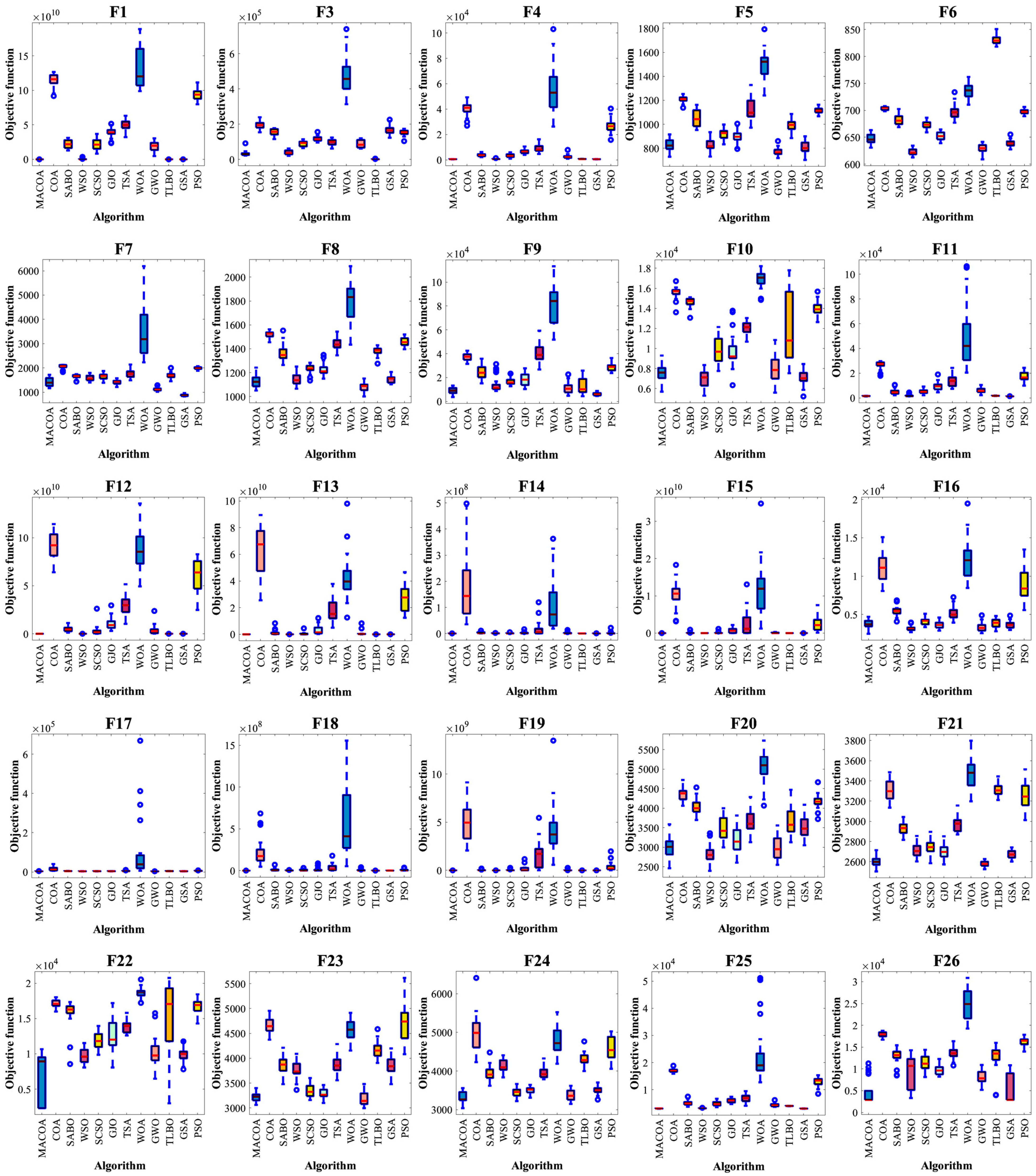
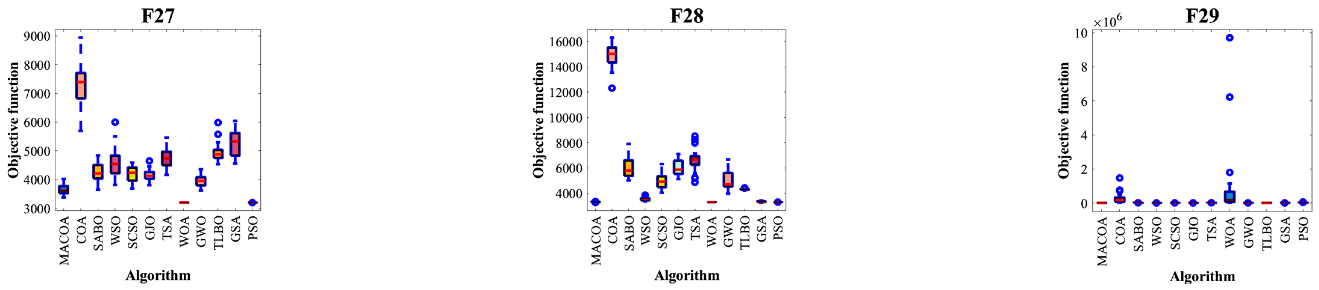
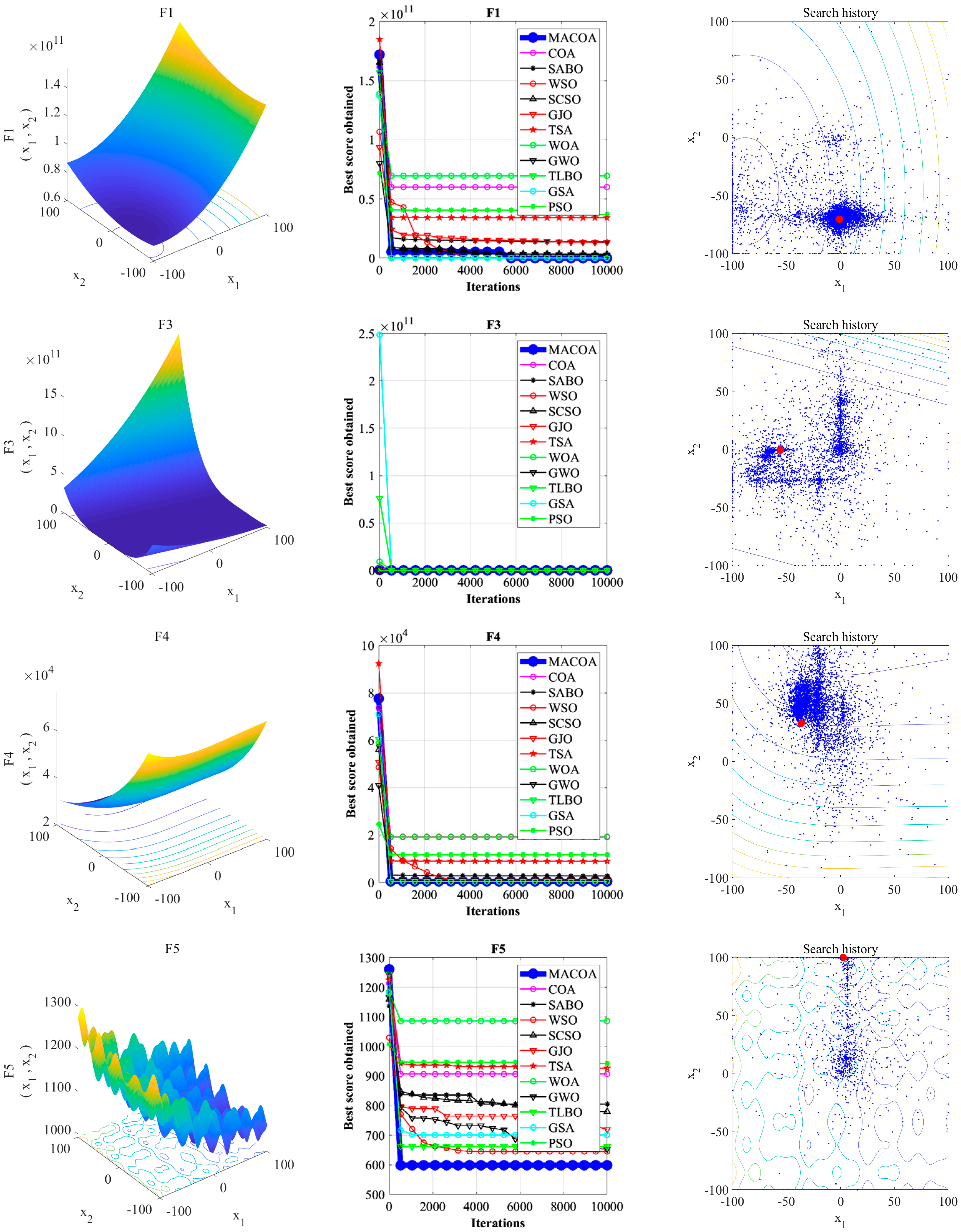
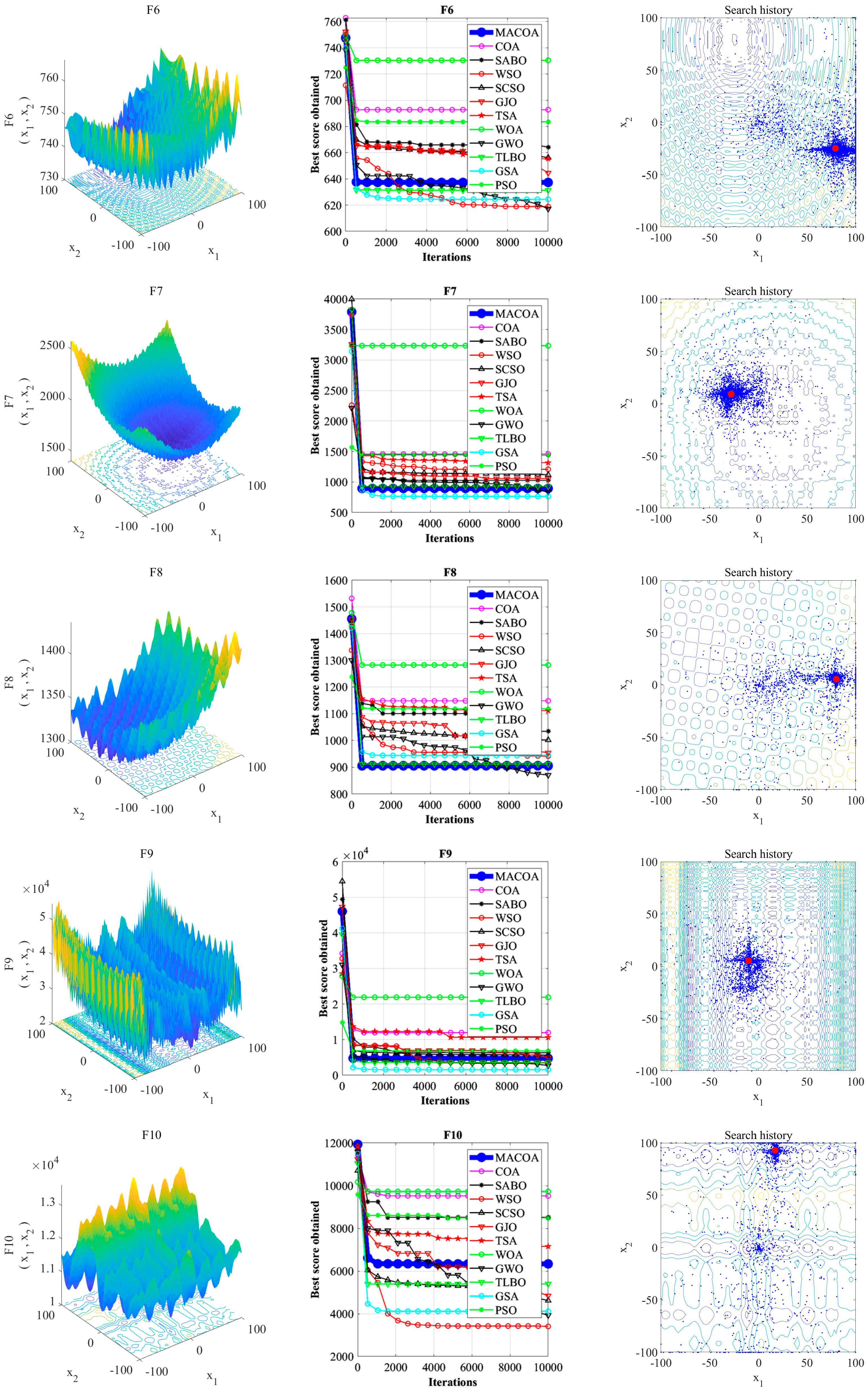
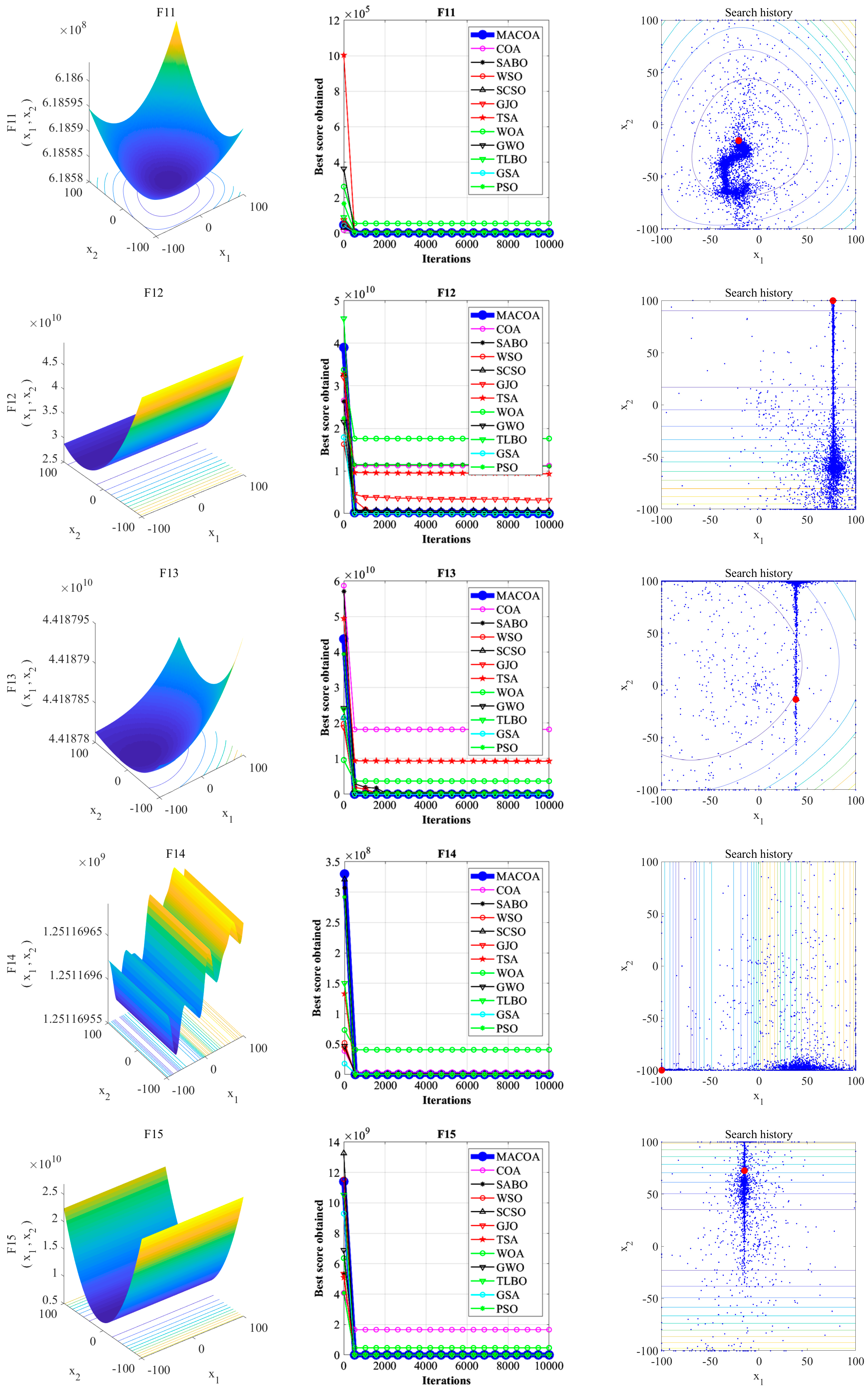
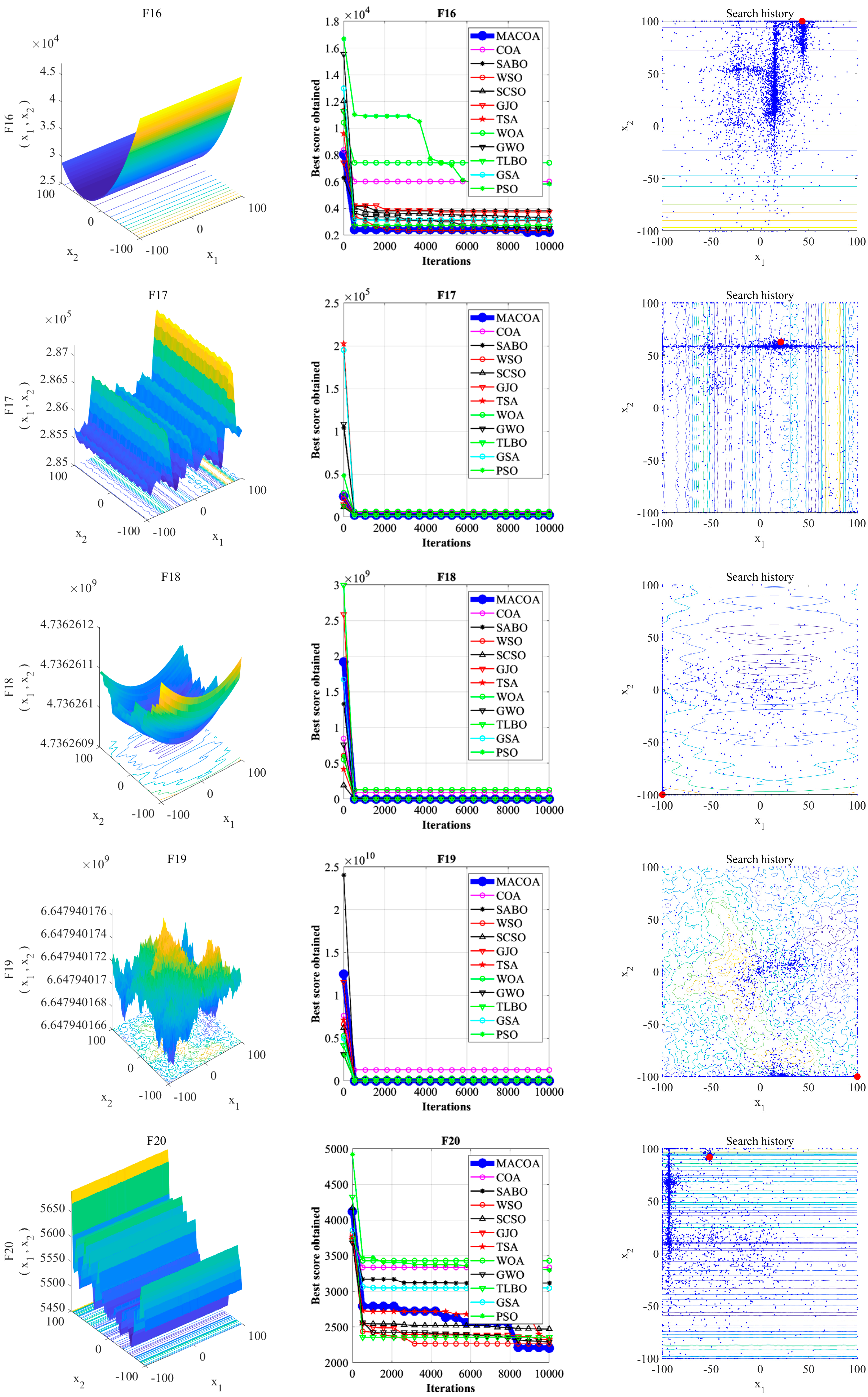
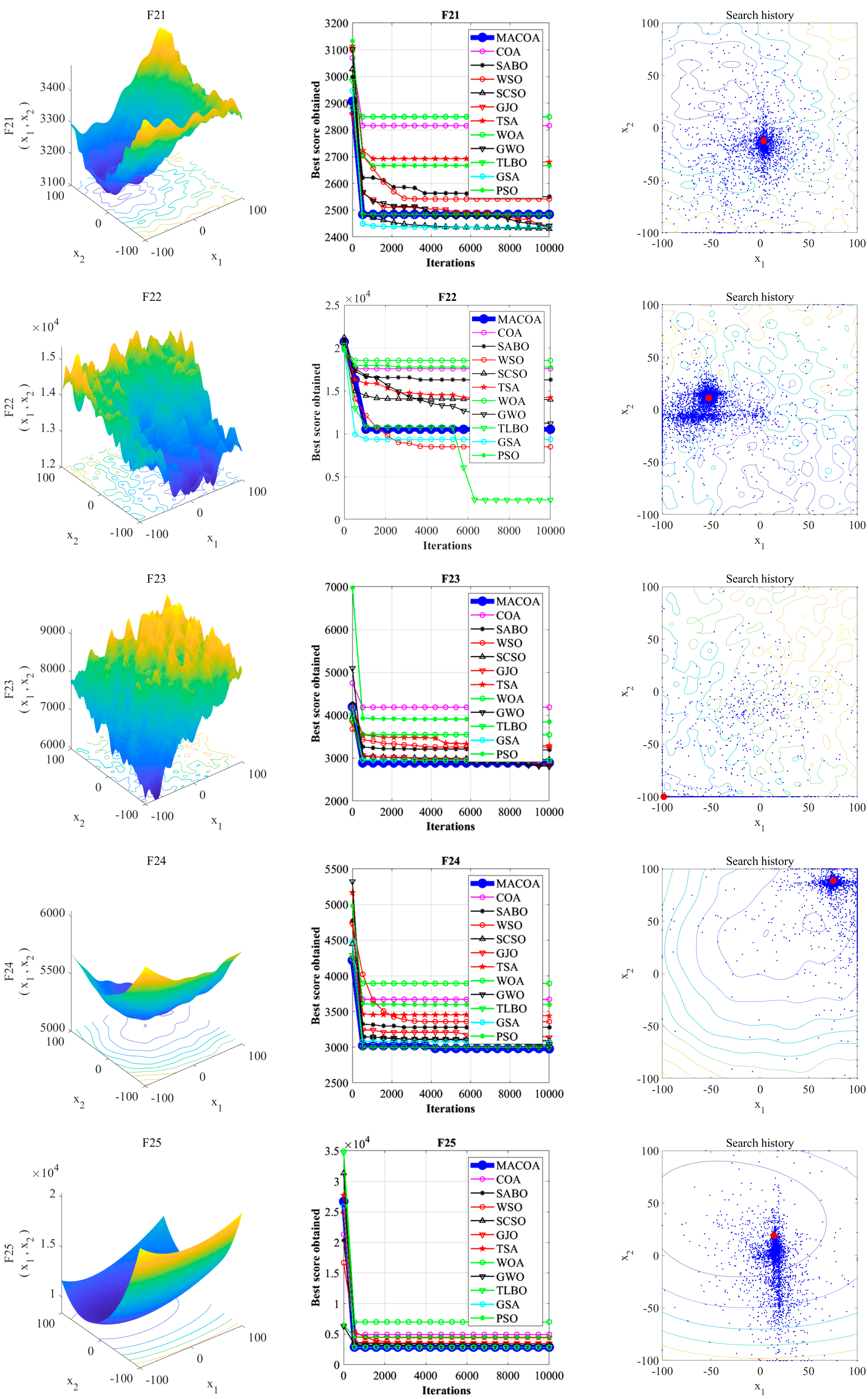
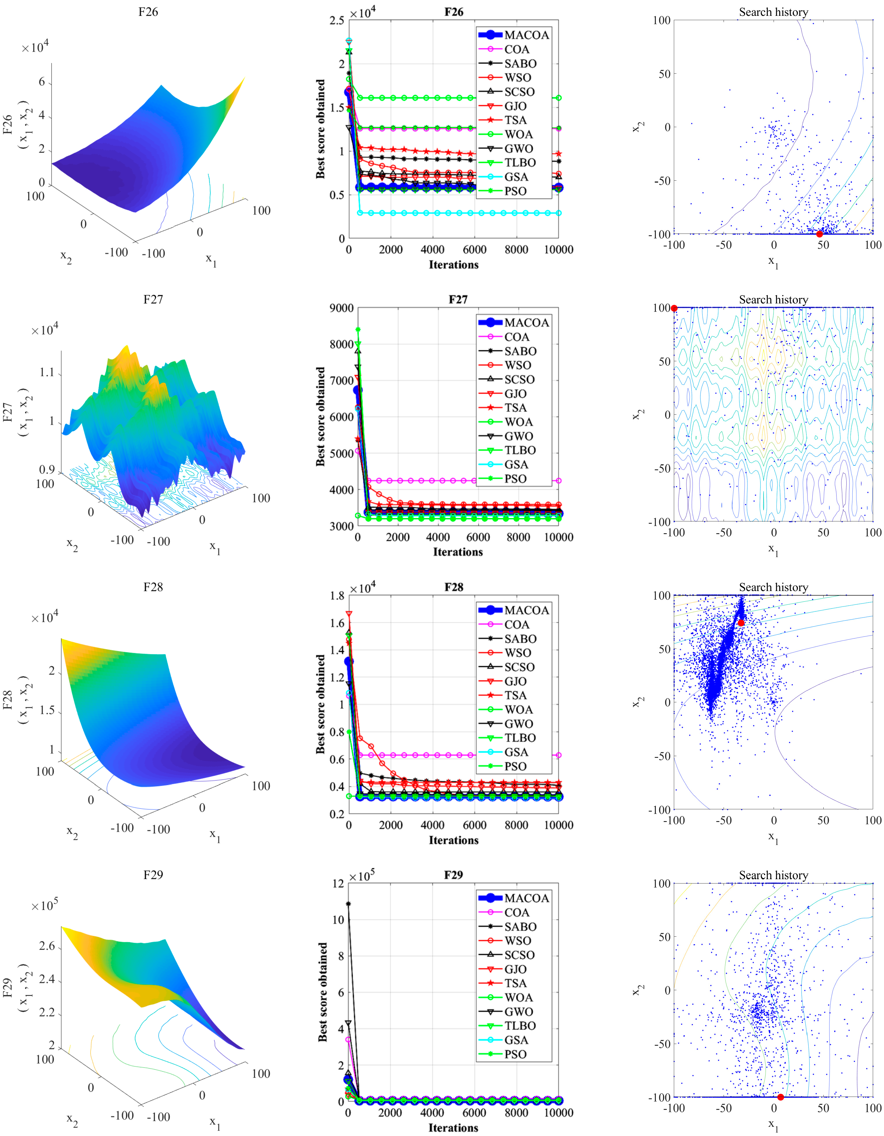
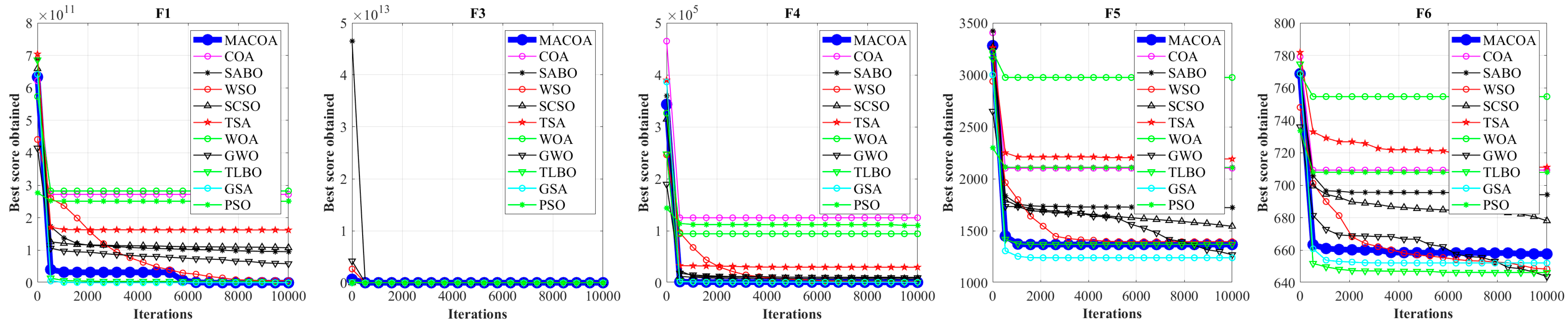
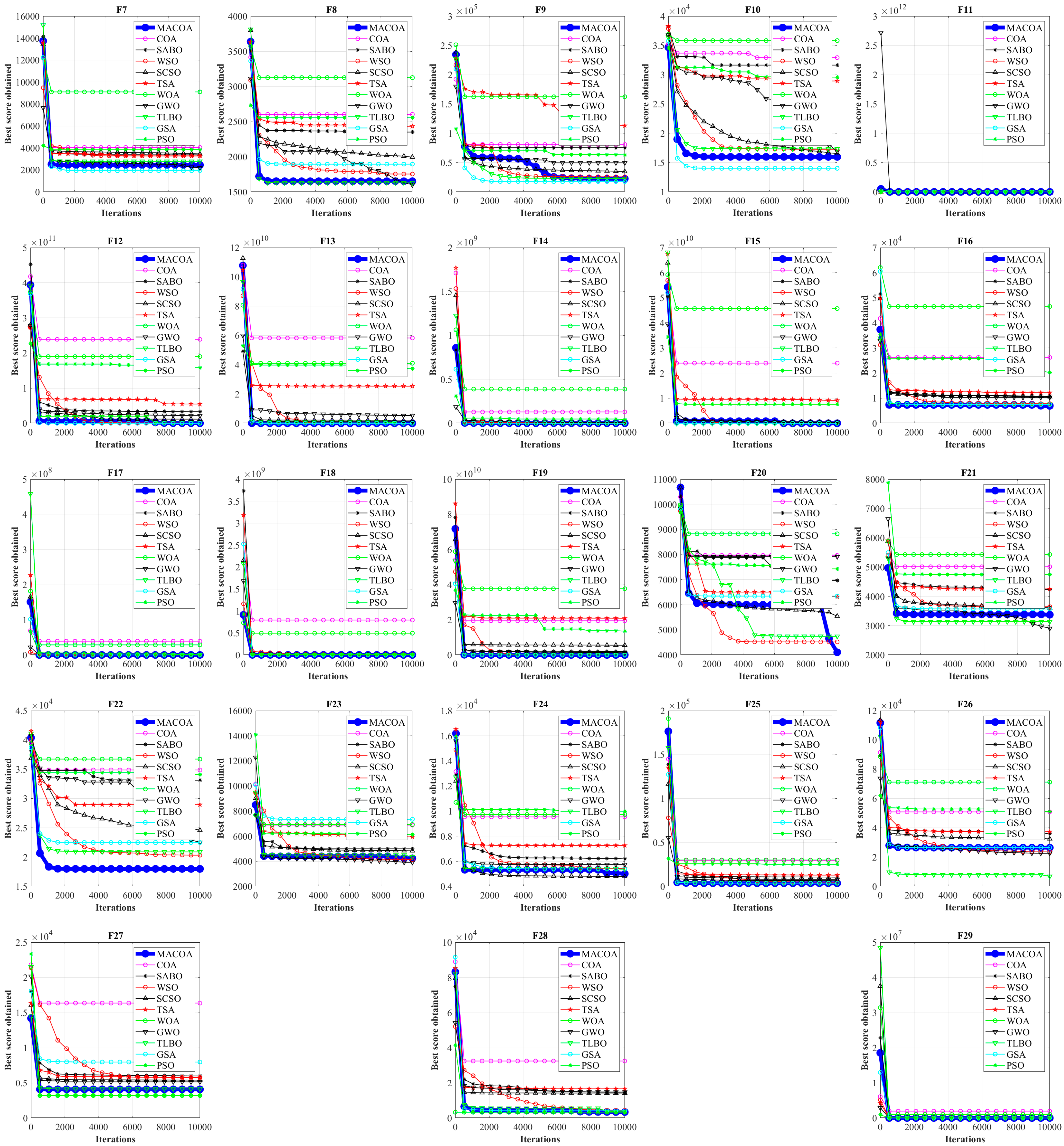
The MACOA searching capability is validated through experimental studies that employ the IEEE CEC2017 benchmark functions. The MACOA is compared with 10 popular algorithms across various dimensions (30, 50, and 100), respectively. A comparative analysis of the convergence curves for all 12 algorithms across these dimensions, along with an examination of boxplots representing the outcomes from multiple runs and search history graphs, reveals that the MACOA demonstrates better optimization results over the other algorithms. To further study the engineering applicability of the MACOA, seven engineering challenges, including the design of a gear train, a reducer, etc., are used to test the ability of MACOA’s optimization. The analysis of the experiment results for these engineering design problems confirms the practical efficacy of the MACOA in optimizing practical engineering problems.

2. Basic Theory

The COA is inspired by the behavior of long-nosed coatis [5]. Each individual coati is a candidate solution. They have two natural behaviors in the hunting period: (1) behaviors when hunting for iguanas, and (2) behaviors when escaping from predators. It can be interpreted as two phases: exploration and exploitation.

2.1. Hunting for Iguanas (Exploration)

During the exploration phase, the coatis initiate a hunt and attack on the iguana, with some coatis climbing a tree in order to get close to the iguana. Other coatis wait beneath the tree to hunt the iguana once it falls to the ground. This strategy enables individual coatis to relocate to various locations within the search space, which showcases the global search capability of the COA within the problem space, i.e., exploration.
During the exploration phase, x b e s t t represents the position of the best individual in the population, corresponding to the iguana location. Half of the coatis will make their way up the tree, and the other half will stay in their original location. They will be waiting for the iguana to come down. The position of the first half is shown in (1):
x i t + 1 ( j ) = x i t ( j ) + r ( x b e s t t ( j ) R I x i t ( j ) ) ,   i = 1 , 2 , , N 2 , j = 1 , 2 , , M
where x i t ( j ) expresses the position of an individual, t is defined as the number of the current iteration, and r is in [0, 1]. RI picks 1 or 2 randomly. N is considered the size of the population. M expresses the size of the dimension.
After the iguana’s fall, it is placed randomly. Then, the coatis, which stay on the ground, move through the space, searching for the iguana. The position is updated by (2) and (3) below:
I g u a n a g r o u n d t ( j ) = l b j + r ( u b j l b j )
x i t + 1 ( j ) = x i t ( j ) + r ( I g u a n a g r o u n d t ( j ) I x i t ( j ) ) , i f   f i t n e s s ( I g u a n a g r o u n d t ) < f i t n e s s ( x i t ) x i t ( j ) + r ( x i t ( j ) I g u a n a g r o u n d t ( j ) ) , e l s e   i = N 2 + 1 , N 2 + 2 , , N
where lbj and ubj express the lower and upper limits of the j-th dimensional variable. fitness(·) is the formula for calculating fitness. I g u a n a g r o u n d t expresses the new position of the iguana after falling. x i t ( j ) is the value of the i-th dimensional variable for the i-th individual under the current iteration.
If the updated location improves the value of the fitness, it is the optional location. Otherwise, the coati remains in its previous position, i.e., a greedy selection is performed in (4).
x i t + 1 = x i t + 1 , i f   f i t n e s s ( x i t + 1 ) < f i t n e s s ( x i t ) x i t , e l s e

2.2. Escaping from Predators (Exploitation)

During the exploitation phase, the updating of the coati’s location was modelled on the natural behavior of a coati escaping from a predator. A coati escapes when a predator comes. The action of the coati in one strategy brings it close to another safe position around its current position, which reflects the local search capability of the COA, i.e., exploitation.
During the exploitation phase, random positions are generated near every coati’s location, as shown in (5) and (6).
l b j l o c a l = l b j t , u b j l o c a l = u b j t , t = 1 , 2 , , T
x i t + 1 ( j ) = x i t ( j ) ( 1 2 r ) ( l b j l o c a l + r ( u b j l o c a l l b j l o c a l ) ) , i = 1 , 2 , , N
where T represents the maximum iteration count. t denotes the current number of iterations. u b j l o c a l and l b j l o c a l express the upper and lower bounds of the j-th dimensional variable, which are updated with each iteration. r is a random value between 0 and 1.
Finally, one more greedy choice is made, i.e., (4).

3. Proposed Algorithm

Although the COA is highly optimized, its initial population is generated randomly. Furthermore, COA employs a random strategy during the hunting phase, and its behavior in avoiding natural enemies is also contingent upon this random approach. These factors contribute to an imbalance between the global search capabilities and local optimization abilities of COA, making it susceptible to converging on local optima, exhibiting limited global exploration capacity, and demonstrating poor convergence accuracy. To address these issues, we propose the following heuristic strategies.

3.1. Chaos Mapping for Lévy Flight

Conventional random strategies generate populations with certain drawbacks, such as a lack of population diversity, and their randomness may lead to the possibility that certain areas are over-explored. Therefore, a mapping process for randomly generated populations is necessary.
The chaotic mapping mechanism is highly uncertain and sensitive. It can generate complicated and unpredictable dynamic behaviors to achieve a broader range of exploration in the search space [26].
Lévy flight is a special random walk model that describes movement patterns with long-tailed distributions [27]. The mapping is used in optimization algorithms to improve the randomness, which can assist the algorithm in more effectively exploring the solution space. Therefore, the global optimization capability is increased [28]. Lévy flights are introduced in the initialization process of the MACOA, as shown in (7)–(9).
α L e v i ( β ) ~ 0.01 u v β X ( t ) X α ( t )
σ u = Γ ( 1 + β ) sin ( π β 2 ) Γ ( 1 + β 2 ) β × 2 β 1 2 1 β , σ v = 1
X ( t + 1 ) = X ( t ) + α L e v i ( β )
where X(t) denotes the location of the i-th coati, and α is the weight of the control step. u ~ N ( 0 , σ u 2 ) . v ~ N ( 0 , σ v 2 ) . β is a constant, which is 1.5.

3.2. Nonlinear Inertia Step Size Factor

In the global optimization phase, premature convergence can hinder the algorithm’s ability to identify the global optimal solution. The incorporation of a nonlinear inertia step factor can mitigate the risk of premature convergence to local optima by dynamically adjusting the step size, thereby preserving the diversity of the population.
The introduction of a nonlinear inertia step size factor can greatly improve search efficiency and convergence performance, and the COA can dynamically adjust individuals’ search behavior. This dynamic adjustment mechanism effectively enhances the balance between exploration and exploitation. It also enhances adaptability and robustness.
Considering that updating a coati’s position is related to a coati’s current position, a nonlinear inertia step size factor is introduced. The factor adjusts the relationship between the coati’s position update and the current position information, depending on the individual coati’s position. Then, the factor is calculated by (10):
ω = ( t T ) C n ( t T ) C n + ( 1 t T ) C n
where Cn is a constant greater than 1 to control the degree of nonlinearities, which is taken as 2 in this method.
Initially, the value of ω is small, resulting in the position updates being less influenced by the current position. This facilitates a broader search range for the algorithm and enhances its global exploration capability. As the search process progresses, the value of ω is increasing over time. The effect brought by the current coati position becomes larger, which assists in obtaining the optimal solution. Furthermore, it enhances the convergence speed as well as its local exploration ability.
The improved formula for modelling coati positions in the first stage is shown in (11):
x i t + 1 ( j ) = ω x i t ( j ) + r ( x b e s t t ( j ) I x i t ( j ) ) ,   i = 1 , 2 , , N 2

3.3. Coati Vigilante Mechanism

In the local optimal search phase, the algorithm usually focuses on a certain region for detailed search. The vigilante mechanism can assist the algorithm in escaping local optima by introducing random perturbations or altering the direction of the search to enhance the algorithm’s exploration.
In the sparrow search algorithm, when part of the sparrows search for food, some of them act as vigilantes, responsible for monitoring the security of their surroundings and sounding an alarm when a potential threat is detected.
This mechanism not only improves the survival rate of the group but also facilitates the rapid dissemination of information. The introduction of the vigilante mechanism enables the algorithm to cope with complex optimization problems more effectively. In this way, the COA can maintain a higher degree of flexibility and dynamism in exploring the solution space [29].
Introducing the sparrow vigilante mechanism in the exploitation phase enhances the vigilance ability of the COA to search within an optional range. The coatis on the outskirts of the population will swiftly relocate to seek a safe area when they realize there is danger. The coati located in the center will walk around randomly in order to get close to others in the population. The sparrow vigilant mechanism formula is shown in (12).
X i , j t + 1 = X b e s t t + β X i , j t X b e s t t , i f   f i > f g X i , j t + K ( X i , j t X w o r s t t ( f i f W ) + ε ) , i f   f i = f g
where X b e s t t represents the global optimal position in the current iteration, and β represents the step control parameter. β ~ N ( 0 , 1 ) . K is randomly selected in [−1, 1]. f i is the fitness value. f g is the greatest global greatest fitness value, and f w is the worst one. ε is a very small constant.
Equation (12) can be optimized to address the problem of the global search capability. A dynamically adjusted step factor [30] is introduced, as shown in (13).
X i , j t + 1 = X b e s t t + β ( t ) X i , j t X b e s t t ,   i f   f i > f g X i , j t + K ( t ) ( X i , j t X w o r s t t ( f i f W ) + ε ) ,   i f   f i = f g
β ( t ) = f g ( f g f w ) ( T t T ) 1.5
K ( t ) = ( f g f w ) e 20 tan ( t T ) 2 ( 2 r a n d 1 )
where β ( t ) is a dynamically adjusted step factor, as shown in (14). K ( t ) is a dynamically adjusted step factor, as shown in (15). r a n d [ 0 , 1 ] .
The introduction of dynamic step factors β ( t ) and K ( t ) enables the algorithm to adjust the search behavior dynamically. At the beginning of the algorithm, it focuses on exploration, and the later phase focuses on exploitation. These optimizations improve the adaptability and robustness of the COA.

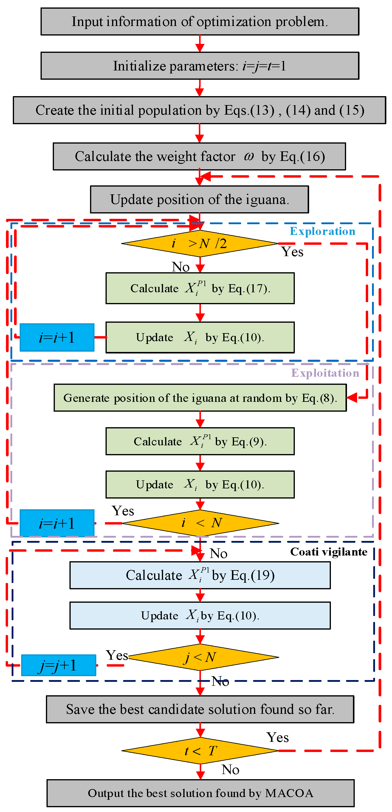
3.4. Multi-Strategy Adaptive Coati Optimization Algorithm

The detailed flowchart of the MACOA is presented in Figure 1. The pseudo-code for MACOA is given in Table 1.

4. Experiments

Simulation studies and evaluations of the optimization efficiency for MACOA are presented. All experiments are conducted on an AMD 64-bit R7 processor operating at 3.20 GHz with 16 GB of RAM, utilizing MATLAB R2018a. This section uses tables that rank the optimal values produced by the algorithms, iteration curves from 10,000 iterations, and box plots from 50 experiments for statistical analysis.

4.1. Benchmark Functions and Compared Algorithms

Twenty-nine standard benchmark functions from the IEEE CEC-2017 [31] are utilized to test MACOA’s capability in addressing various objective functions. A comparison of MACOA’s performance with eleven well-known algorithms is performed in order to assess its quality in providing optimal solutions, namely COA, SABO [32], WSO [33], SCSO [34], GJO [35], TSA [36], WOA [37], GWO [38], TLBO [39], GSA [40], and PSO [41].
The results are presented through four metrics: mean, standard deviation (std), rank, and execution time (ET). The control parameter values for all compared algorithms are specified in Table 2.

4.2. Complexity Analysis

The complexity analysis of the algorithms was carried out using the problem definition and evaluation criteria of the CEC2017 Special Session and Competition on the Complexity of Single-Objective Constrained Numerical Optimisation Algorithms [42]. The steps are as follows:
(1)
Calculate the system running time T0 by running the following test procedure:
x = 0.05
for i = 1:10,000
x = x; x = x/2; x = x×x; x = sqrt(x);
x = log(x); x = exp(x); x = x/(x + 2)
end
(2)
Calculate the complete computing time with 100,000 evaluations of the same D-dimensional function, i.e., T1.
(3)
Calculate the complete computing time for the algorithm with 100,000 evaluations of the same D-dimensional function, i.e., T2.
(4)
The complexity of the algorithm is reflected by (T2T1)/T0.
In this section, the algorithmic complexity analysis of MACOA, along with the other 11 algorithms in running the CEC2017 test function, is performed. In step (2), the maximum number of iterations is set to 10,000, and the number of dimensions is chosen to be 10. In step (3), the number of dimensions is set to 30. Table 3 lists the algorithmic complexity of each algorithm for running the CEC2017 functions. As can be seen from Table 3, the MACOA algorithm computes the function with increased time complexity compared to the COA algorithm, but the optimization performance is significantly improved over the COA algorithm. At the same time, from the point of view of the time complexity values of different algorithms for calculating the functions in CEC2017, the MACOA algorithm ranks in the middle in terms of the time complexity.
In the space complexity analysis, pop is the population size, dim is the dimension of the problem, and Max is the maximum number of iterations. From Table 4, it can be seen that MACOA does not improve the space complexity but improves the accuracy compared to COA.

4.3. Experimental Results and Analysis

CEC-2017 includes thirty standard benchmark functions of various types, as shown in Table 5. The test function F2 from the CEC-2017 is not used in this paper because of its unstable performance (as noted by other authors in their paper [19]). Complete information and details for these test functions can be found in Reference [31].
The proposed MACOA is subjected to 29 independent experiments at CEC-2017, each containing 200,000 FEs. Three dimensions of test functions are used in the experiments: 30, 50, and 100.
The box plots in Figure 2 illustrate the distribution of results from 50 experiments. Based on the box-and-line plot, it can be seen that MACOA produces few outliers compared to other algorithms and achieves the optimal value for all algorithms in most of the tested functions. Therefore, MACOA has strong convergence and stability.
The 3D Surface Plots of CEC2017, iterative curves of the comparison algorithms, and search history plots are shown in Figure 3. According to the search history from Figure 3, the population distribution of MACOA is mostly located near the global optimal solution, and the overall convergence performance of the population is good.
Figure 3 and Figure 4 illustrate the convergence curves of MACOA and the compared algorithms after 10,000 iterations across the 29 benchmark functions from IEEE CEC2017. It is evident that MACOA exhibits a quicker convergence speed and superior convergence performance in comparison to other algorithms.
Additionally, the results are presented in Table 6, Table 7 and Table 8. The results for dimension 30 (m = 30) show that the MACOA is the best algorithm for solving F4, F10, F11, F22, F24~F26, F28, and F29 functions. The results of dimension 50 (m = 50) describe that MACOA is the best optimization algorithm for solving the F1, F4, F10, F11, F16, F18, F22~F26, and F29 functions. From the results for dimension 100 (m = 100), it can be obtained that MACOA is the best optimization algorithm for solving F1, F4, F10, F12, F14, F16, F17, F22~F26, F29, and F30 functions. Therefore, MACOA outperforms the comparison algorithms for most of the tested functions. Overall, MACOA works best in different dimensions (30, 50, and 100) of the CEC-2017 tested functions.
In comparison to the other 11 algorithms, the MACOA proposed has strong exploration, exploitation, and search capability. It shows improved performance compared to other optimization algorithms.

4.4. Ablation Experiment

In order to analyze the impact of different strategies on the performance of the algorithm, this section compares three strategies of MACOA through experimental analysis. In this section, the experiments are conducted using the test function of CEC2017, with all other parameters kept the same as before, and only the optimal value is used as the evaluation index. The results of the optimization study are shown in Table 9. L refers to Lévy flight, N refers to the nonlinear inertial step factor, and V refers to the coati vigilante mechanism.
From Table 9, it can be seen that the MACOA optimization with the introduction of the three strategies is the best. The second is COA + L + V with Levi flight and coati vigilante mechanism improvement. The third is nonlinear inertial step factor and vigilante mechanism improvement. All algorithms outperform the original COA. However, the results of COA + V and COA + L + N show that the coati vigilante mechanism works better than the other two strategies. In conclusion, all three improved strategies positively affect the original algorithm, proving the effectiveness of the heuristic strategy.

5. Engineering Problems

A benchmark suite of real-world non-convex constrained optimization problems and various established baseline results are utilized to analyze the engineering problems. In these constrained engineering problem designs, we use penalty terms as constraints. The optimization algorithm will find the global optimal solution under the constraints to achieve the constrained design. Problem difficulty within the benchmark is assessed using various evaluation criteria [43]. The algorithms COA, SABO, WSO, SCSO, GJO, TSA, SRS [44], MPA [45], and TLBO are included for comparative analysis, with each algorithm executed independently for 50 runs on all problems within the benchmark suite. Performance is evaluated based on feasibility rate (FR) and success rate (SR). FR represents the proportion of runs achieving at least one feasible solution within the maximum function evaluations. Meanwhile, SR denotes the proportion of runs where a feasible solution x satisfies f(x) − f(x*) ≤ 10−8 within function evaluations. This section uses tables of optimal, standard deviation, mean, median, worst, FR, and SR values generated by the algorithms, iteration curves generated by 10,000 iterations, box plots generated by 50 experiments, and search history for statistical analysis.

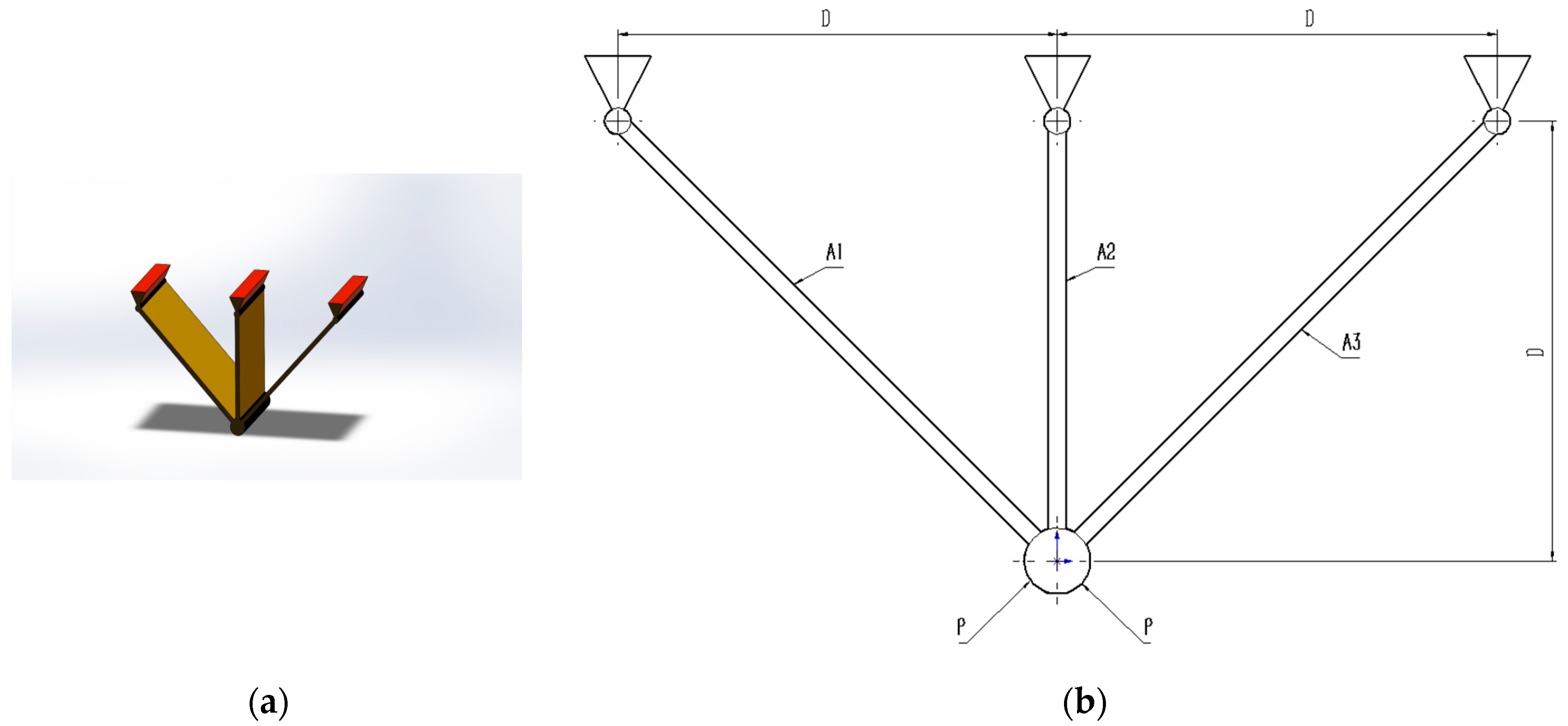
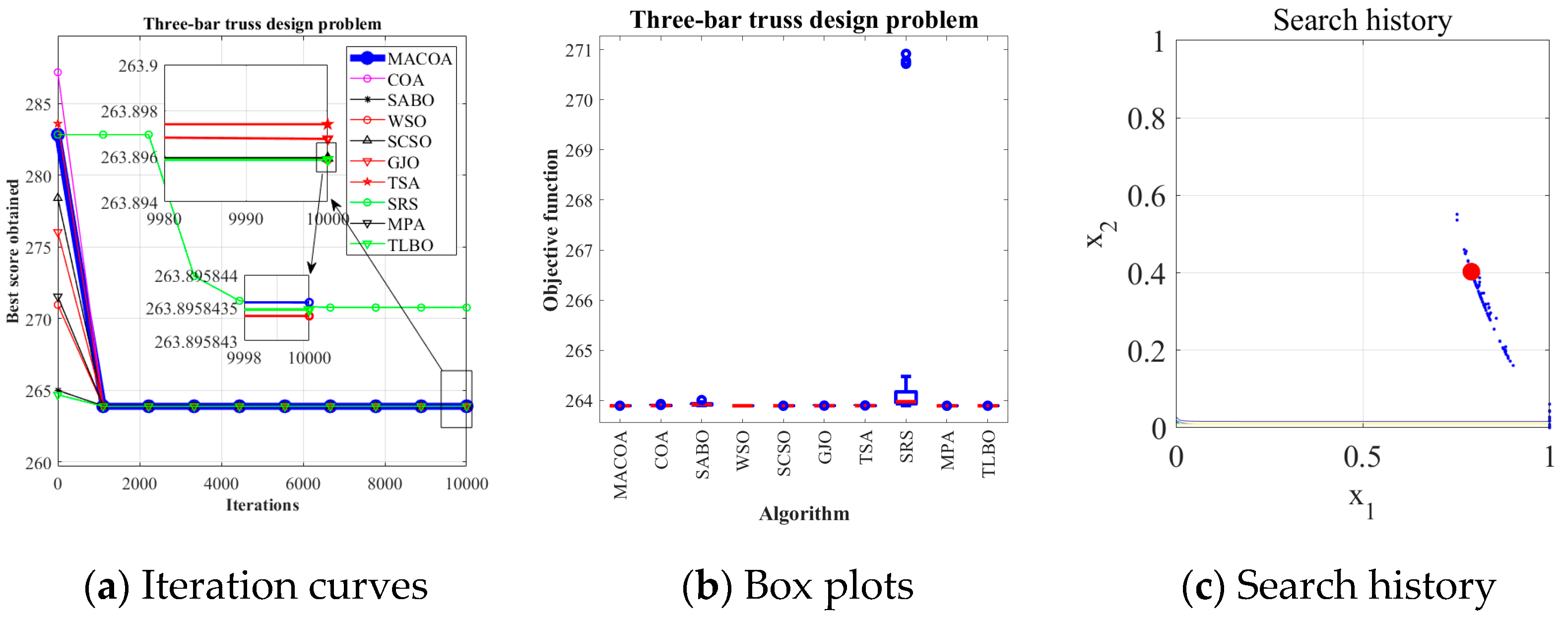
5.1. Three-Bar Truss Design Problem

The three-bar truss design problem is to minimize the volume while satisfying the stress constraints on each side of the truss member. Figure 5 provides the geometry explanation. Within the benchmark suite, the problem features D = 2 decision variables, g = 3 inequality constraints, and h = 0 equality constraints. The optimal value of the objective function is known to be f(x*) = 2.6389584338 × 10² [43].
The design problem for the three-bar truss can be outlined as follows:
Consider
x = [ x 1   x 2 ] = [ A 1   A 2 ]
Objective function:
f ( x ) = ( 2 2 x 1 + x 2 ) l
Subject to
g 1 ( x ) = 2 x 1 + x 2 2 x 1 2 + 2 x 1 x 2 P σ 0
g 2 ( x ) = x 2 2 x 1 2 + 2 x 1 x 2 P σ 0
g 3 ( x ) = 1 2 x 2 + x 1 P σ 0
where
l = 100   cm , P = 2   kN / cm 3 , σ = 2   kN / cm 3
Boundaries:
0 x 1 1
0 x 2 1
From the experimental results in Table 10, it can be seen that MACOA has FR = 2 and SR = 10. These results show that MACOA’s FR score is second only to MPA, while its SR value is second only to MPA and TLBO. Moreover, the results of MACOA are significantly better than COA. Figure 6a illustrates the iteration process of the optimal solutions of the ten algorithms. The box-and-line plot is displayed in Figure 6b, and it can be seen that MACOA has strong stability. Figure 6c shows the search history, from which it can be seen that the search history of MACOA is concentrated around this neighborhood of the global optimal solution. Overall, these results show that MACOA outperforms COA.

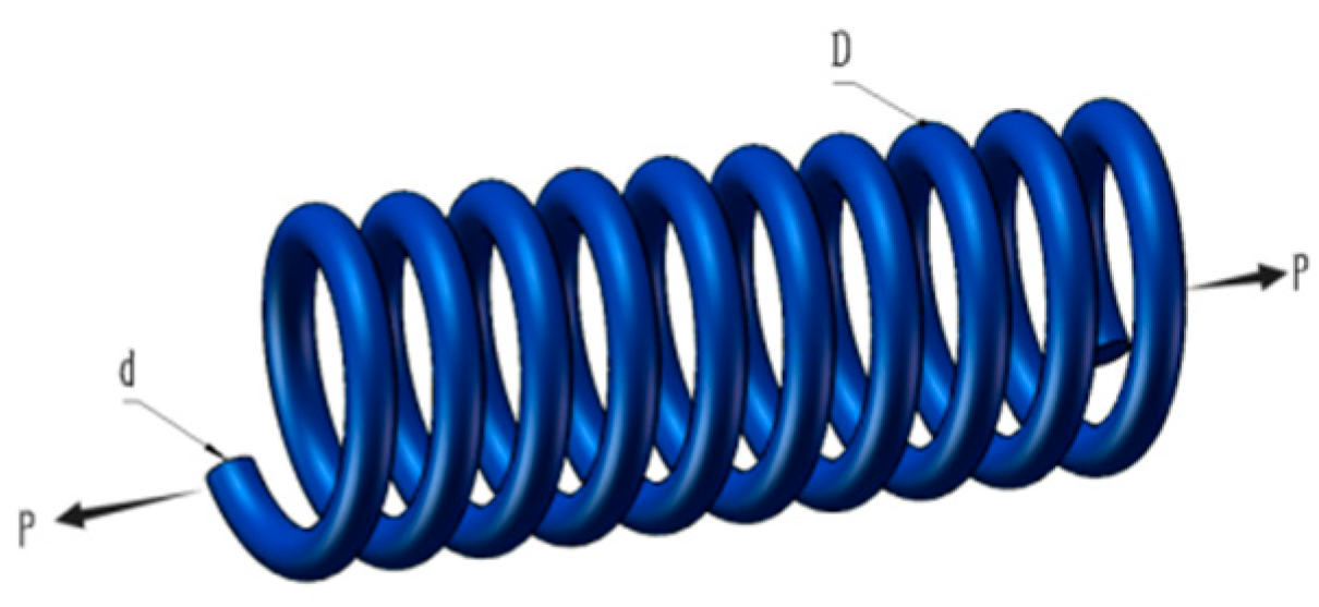
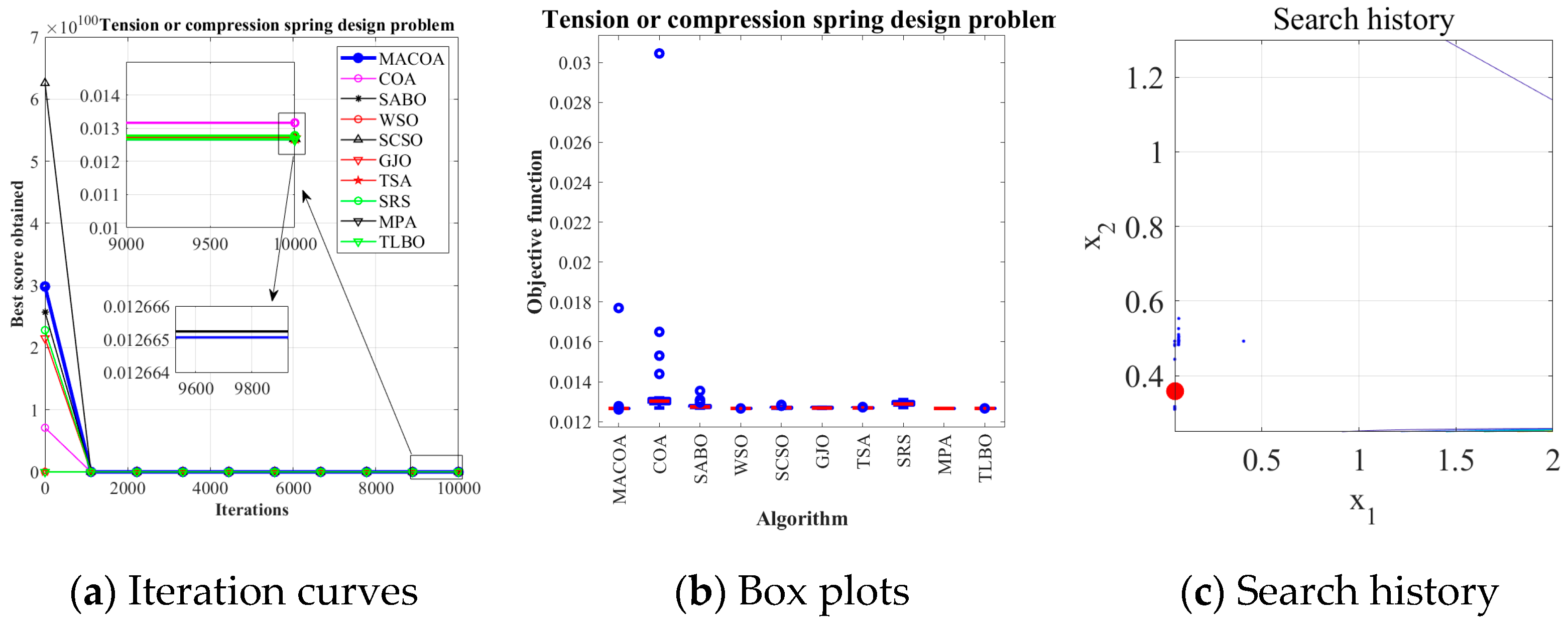
5.2. Tension or Compression Spring Design Problem

The design of tension or compression springs represents a common optimization problem in mechanical engineering and structural design. The function of this device is to store and discharge energy.
Therefore, a spring requires consideration of parameters during the design process. Within the benchmark suite, the problem features D = 3 decision variables, g = 4 inequality constraints, and h = 0 equality constraints. The optimal value of the objective function is known to be f(x*) = 1.2665232788 × 10⁻² within the benchmark [43]. Figure 7 illustrates the pressure vessel configuration.
The design problem for tension or compression springs can be outlined as follows:
Consider
x = [ x 1   x 2   x 3 ] = [ d D N ]
Objective function:
f ( x ) = ( x 3 + 2 ) × x 2 × x 1 2
Subject to
g 1 ( x ) = 1 x 3 × x 2 3 71785 × x 1 4 0
g 2 ( x ) = 4 × x 2 2 x 1 × x 2 12566 × ( x 2 × x 1 3 x 1 4 ) + 1 5108 × x 1 2 1 0
g 3 ( x ) = 1 140.45 × x 1 x 2 2 × x 3 0
g 4 ( x ) = x 1 + x 2 1.5 1 0
Boundaries:
0.05 x 1 2.0
0.25 x 2 1.3
2.0 x 3 15.0
The experimental results in Table 11 show that MACOA has an FR of 98 and an SR of 98. These results indicate that MACOA has the highest FR among all the compared algorithms, and its SR is second only to WSO and MPA. Figure 8a illustrates the iteration process of the optimal solutions of the ten algorithms. The box-and-line plot is displayed in Figure 8b. It can be seen that MACOA has very few outliers. Figure 8c shows the search history. Although most of the search range lies on the boundary, it can be seen that most of the search history lies around the global optimum. Overall, these results show that MACOA outperforms COA.

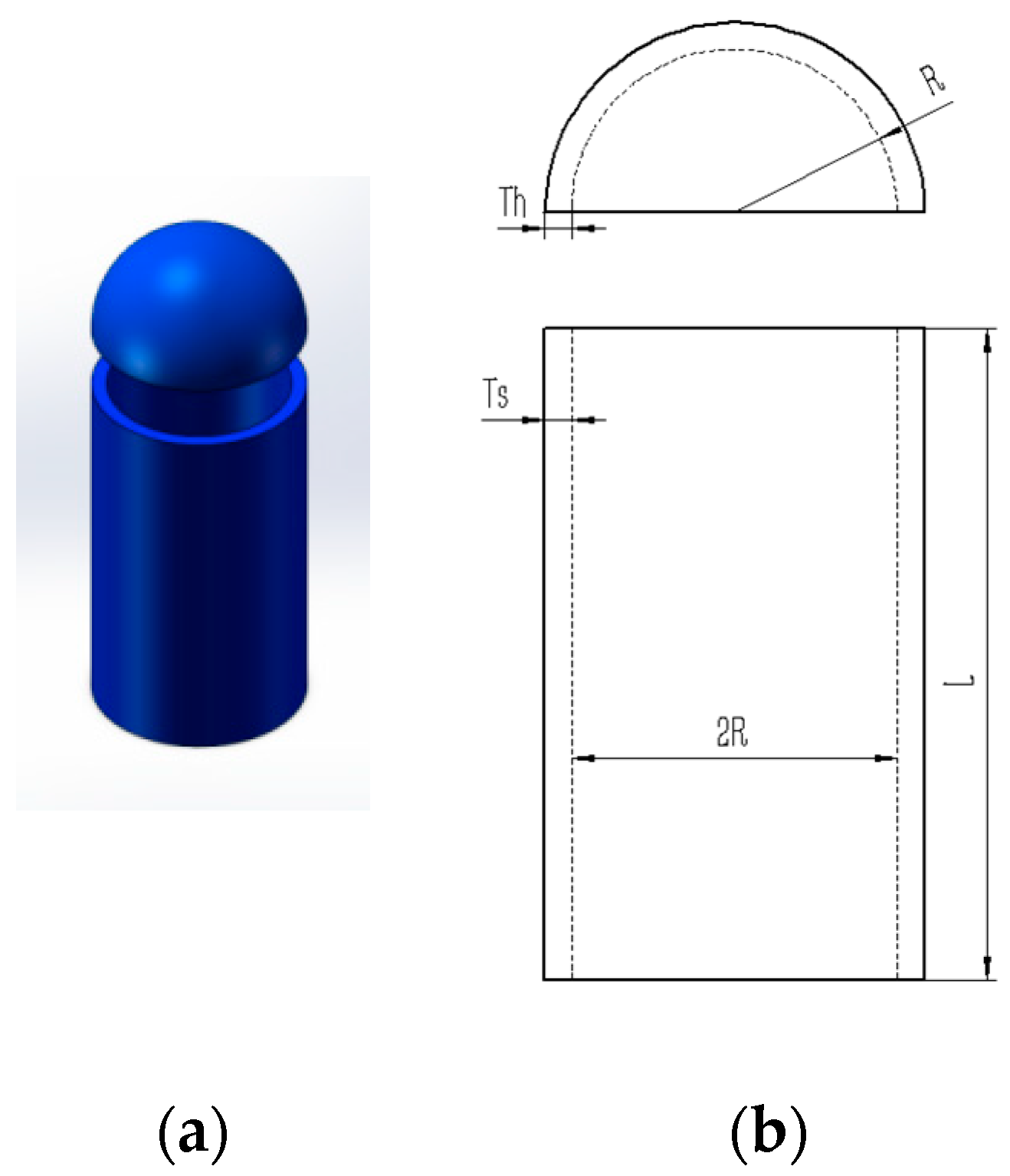
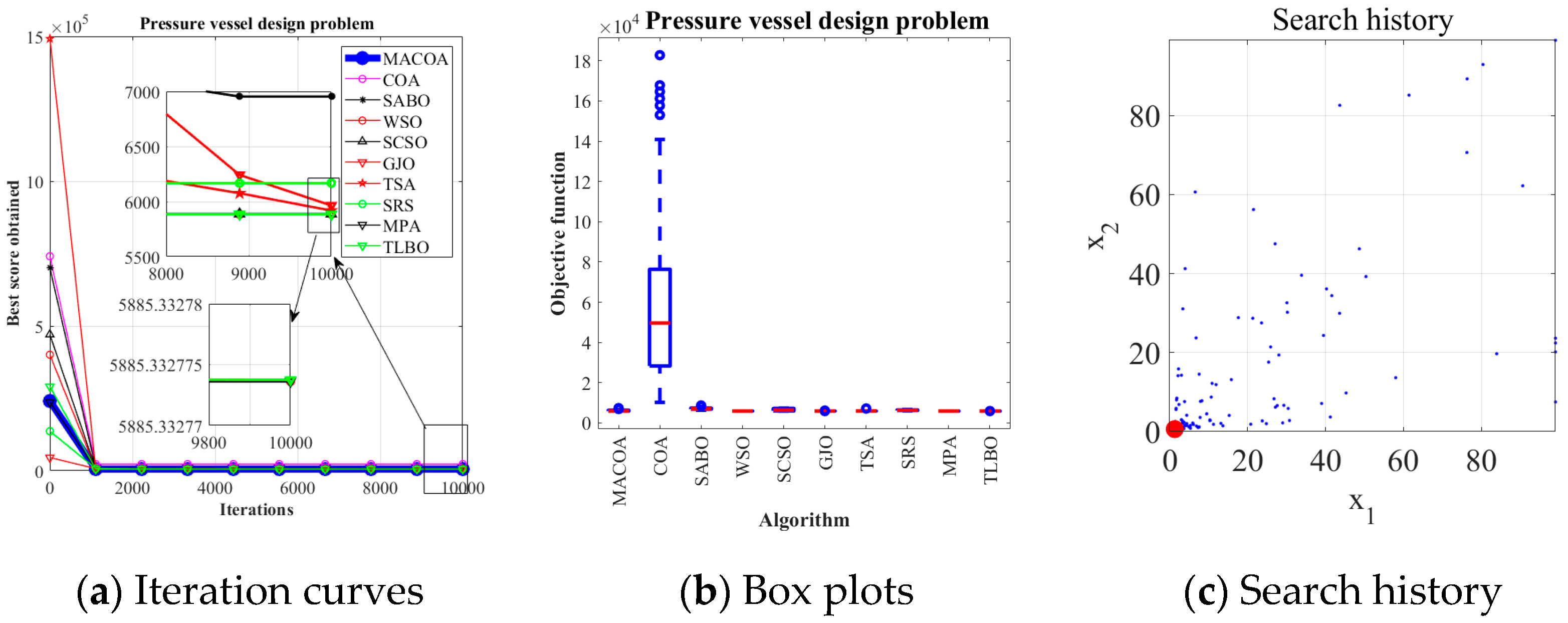
5.3. Pressure Vessel Design Problem

The pressure vessel design problem focuses on minimizing weight while maintaining structural integrity under high-pressure operating conditions. This involves optimizing design parameters, including material selection and wall thickness, within specified constraints to minimize the overall manufacturing costs. Within the benchmark suite, the problem features D = 4 decision variables, g = 4 inequality constraints, and h = 0 equality constraints. The optimal value of the objective function is known to be f(x*) = 5.8853327736 × 10³ [43]. Figure 9 illustrates the pressure vessel configuration. The design problem for the pressure vessel can be outlined as follows:
Consider
x = [ x 1   x 2   x 3   x 4 ] = [ T S   T h   R   L ]
Objective function:
f ( x ) = 0.6224 x 1 x 2 x 3 + 1.7781 x 2 x 3 2 + 3.1661 x 1 2 x 4 + 19.84 x 1 2 x 3
Subject to
g 1 ( x ) = x 1 + 0.0193 x 3 0
g 2 ( x ) = x 3 + 0.00954 x 3 0
g 3 ( x ) = π x 3 2 x 4 + 4 3 π x 3 3 + 1296000 0
g 4 ( x ) = x 4 240 0
Boundaries:
0 x 1 99
0 x 2 99
10 x 3 200
10 x 4 200
The results in Table 12 show that MACOA has the highest FR value among all the algorithms, with both FR and SR values of 98. Meanwhile, the SR value of MACOA is second only to TLBO and MPA. Figure 10a shows the iterative process for the optimal solution of the ten algorithms. Figure 10b, on the other hand, shows the box plots, from which it can be seen that the anomalies and quartiles of MACOA are concentrated with a certain degree of stability. Figure 10c shows the search history of MACOA, from which it can be seen that most of the search history of MACOA is concentrated near the global optimal solution region. These results show that MACOA can obtain the best performances.

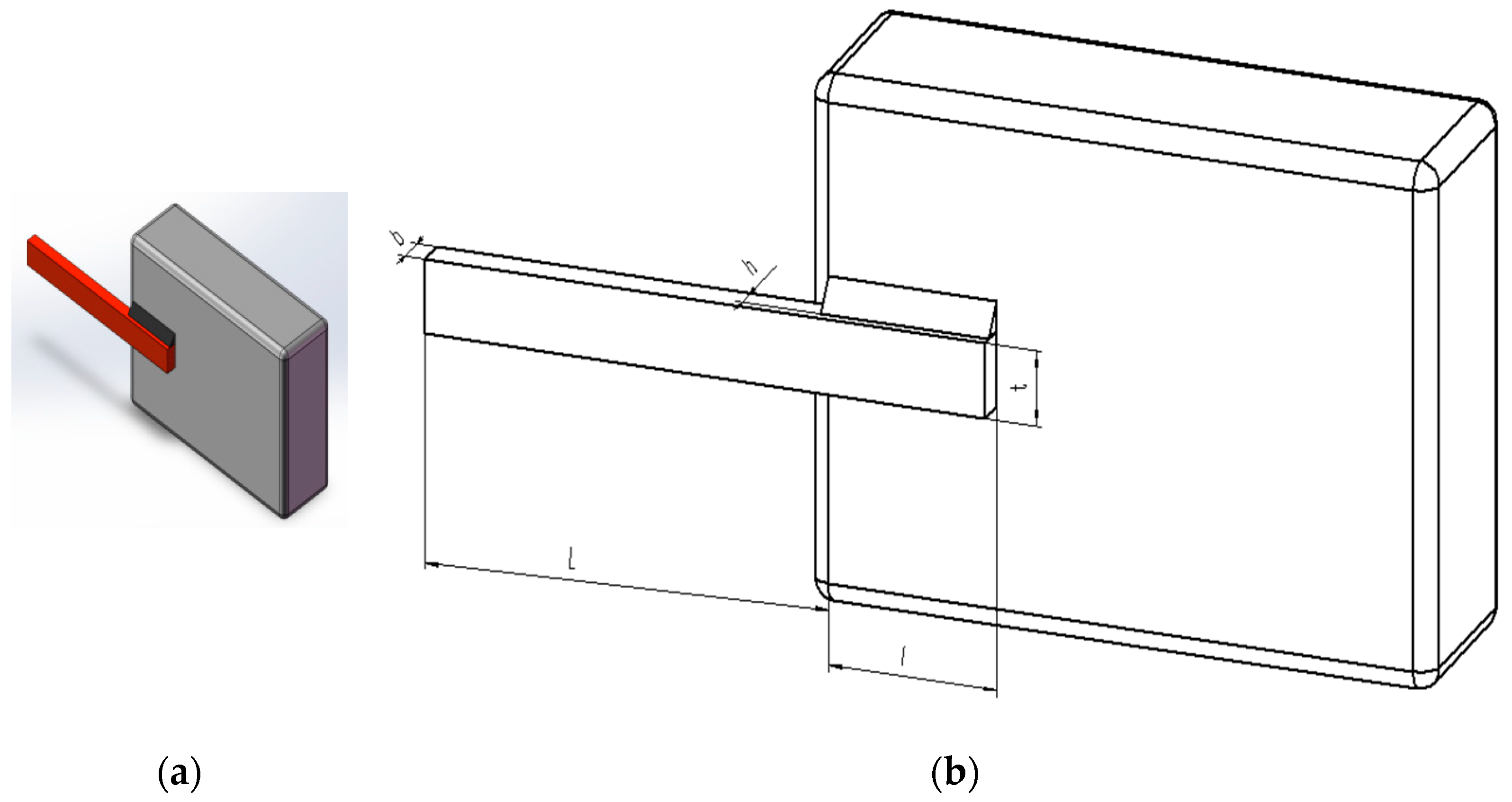
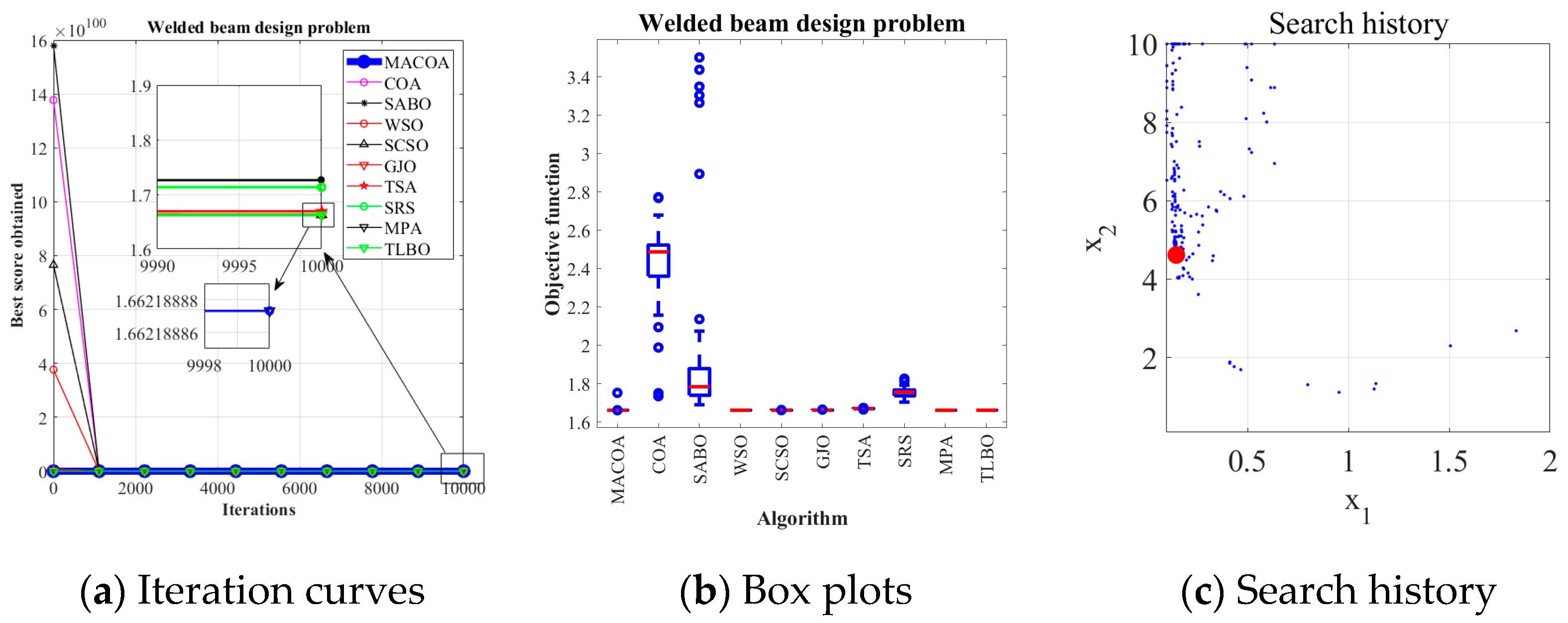
5.4. Welded Beam Design Problem

The welded beam design problem is to maximize structural performance while minimizing the beam’s weight by optimizing parameters such as weld dimensions, geometry, and placement, subject to specific constraints. Within the benchmark suite, the problem features D = 4 decision variables, g = 7 inequality constraints, and h = 0 equality constraints. The optimal value of the objective function is known to be f(x*) = 1.6702177263 [43]. Figure 11 describes the welded beam structure.
The design problem for the welded beam can be outlined as follows:
Consider
x = [ x 1   x 2   x 3   x 4 ] = [ h   l   t   b ]
Objective function:
f ( x ) = 1.10471 x 1 2 x 2 + 0.04811 x 3 x 4 ( 14.0 + x 2 )
Subject to
g 1 ( x ) = τ ( x ) τ max 0
g 2 ( x ) = σ ( x ) σ max 0
g 3 ( x ) = δ ( x ) δ max 0
g 4 ( x ) = x 1 x 4 0
g 5 ( x ) = P P C ( x ) 0
g 6 ( x ) = 0.125 x 1 0
g 7 ( x ) = 1.10471 x 1 2 + 0.04811 x 3 x 4 ( 14.0 + x 2 ) 0.5 0
where
τ ( x ) = ( τ ) 2 + 2 τ τ x 2 2 R + ( τ ) , τ = P 2 x 1 x 2 , τ = M R J
M = P ( L + x 2 2 ) , R = x 2 2 4 + x 1 + x 3 2 2 , σ ( x ) = 6 P L x 4 x 3 2
J = 2 2 x 1 x 2 x 2 2 4 + x 1 + x 3 2 2 , δ ( x ) = 6 P L 3 E x 3 2 x 4
P c ( x ) = 4.013 E x 3 2 x 4 6 / 36 L 2 1 x 3 2 L E 4 G ,
P = 6000 l b , L = 14 i n , δ max = 0.25 i n , E = 30 × 10 6 p s i
τ max = 13600 p s i   a n d   σ max = 30000 p s i
Boundaries:
0.1 x 1 2
0.1 x 2 10
0.1 x 3 10
0.1 x 4 2
The MACOA results in Table 13 show that both FR and SR are 84, which are significantly better than those of COA in both metrics. Figure 12a shows the iterative process of the optimal solutions found by the ten algorithms. Figure 12b shows the boxplots generated from 50 experiments, where MACOA is far superior to COA in terms of the number of anomalies and the median number of anomalies. Figure 12c shows the search history of MACOA, where most of the search histories are clustered around the lower bound. These results clearly show the superior performance of MACOA compared to COA.

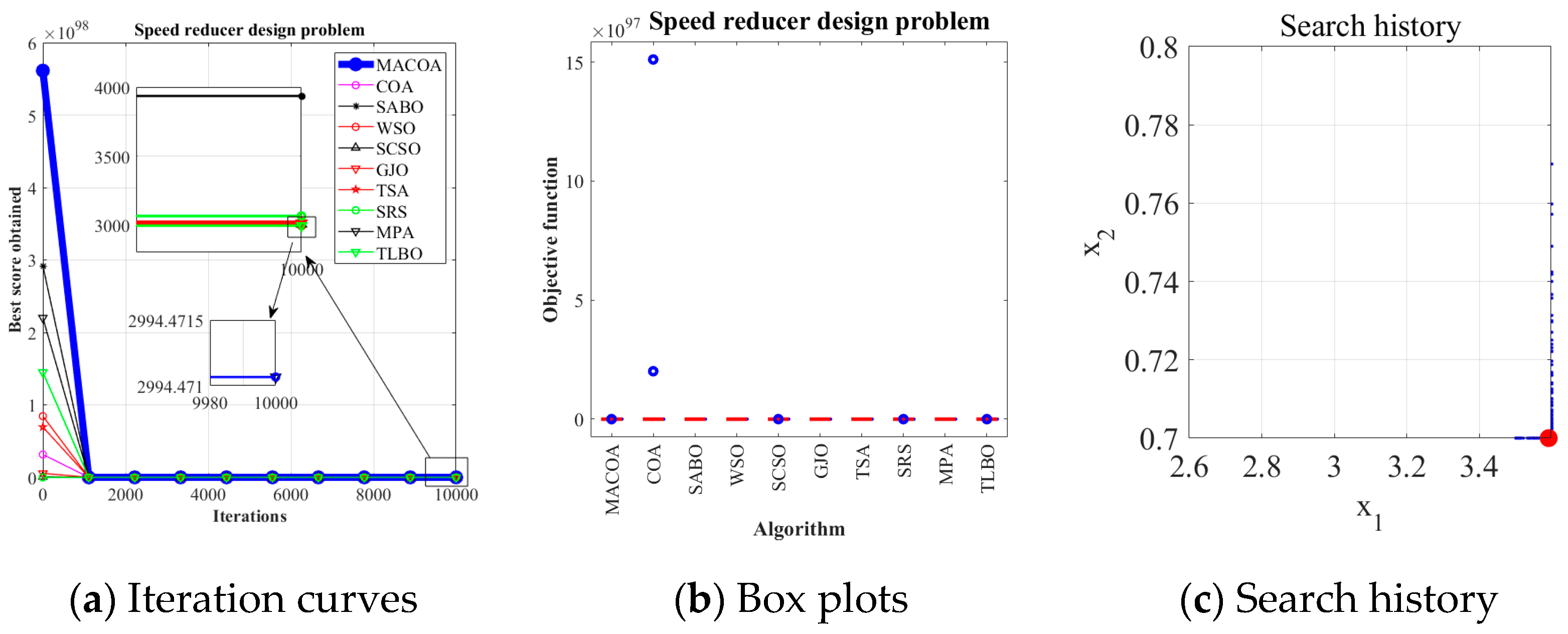
5.5. Speed Reducer Design Problem

The speed reducer design problem is a well-known optimization challenge in engineering design. Within the benchmark suite, the problem features D = 7 decision variables, g = 11 inequality constraints, and h = 0 equality constraints. The optimal value of the objective function is known to be f (x*) = 2.9944 × 10³ [43]. Figure 13 illustrates the speed reducer configuration.
The design problem for the speed reducer can be outlined as follows:
Consider
x = [ x 1   x 2   x 3   x 4   x 5   x 6   x 7 ] = [ b   m   z 2   l 1   l 2   d 1   d 2 ]
Objective function:
f ( X ) = 0.7854 x 1 x 2 2 ( 3.3333 x 3 2 + 14.9334 x 3 43.0934 ) 1.508 x 1 ( x 6 2 + x 7 2 ) + 7.4777 ( x 6 3 + x 7 3 ) + 0.7854 ( x 4 x 6 2 + x 5 x 7 2 )
Subject to
g 1 ( x ) = 27 x 1 x 2 2 x 3 1 0
g 2 ( x ) = 397.5 x 1 x 2 2 x 3 2 1 0
g 3 ( x ) = 1.93 x 4 3 x 2 x 6 4 x 3 1 0
g 4 ( x ) = 1.93 x 5 3 x 2 x 7 4 x 3 1 0
g 5 ( x ) = ( 745 x 4 / ( x 2 x 3 ) ) 2 + 16.9 × 10 6 110 x 6 3 1 0
g 6 ( x ) = ( 745 x 5 / ( x 2 x 3 ) ) 2 + 157.5 × 10 6 85 x 7 3 1 0
g 7 ( x ) = x 2 x 3 40 1 0
g 8 ( x ) = 5 x 2 x 1 1 0
g 9 ( x ) = x 1 12 x 2 1 0
g 10 ( x ) = 1.5 x 6 + 1.9 x 4 1 0
g 11 ( x ) = 1.1 x 7 + 1.9 x 5 1 0
Boundaries:
2.6 x 1 3.6
0.7 x 2 0.8
17 x 3 28
7.3 x 4 8.3
7.8 x 5 8.3
2.9 x 6 3.9
5 x 7 5.5
Table 14 shows that MACOA achieves FR = 46 and SR = 46, which are much higher than those of COA, and although WSO, MPA, and TLBO have slightly better FR and SR values, MACOA still outperforms other algorithms, including COA. Figure 14a shows the iterative process graphs for the optimal solutions of all algorithms. Figure 14b shows the boxplots of 50 experiments, demonstrating that MACOA has far fewer anomalies than COA. Figure 14c shows the search history of MACOA, with most of the search points clustered around the boundary and global optimal solutions. The above analysis can conclude that MACOA is significantly better than COA.

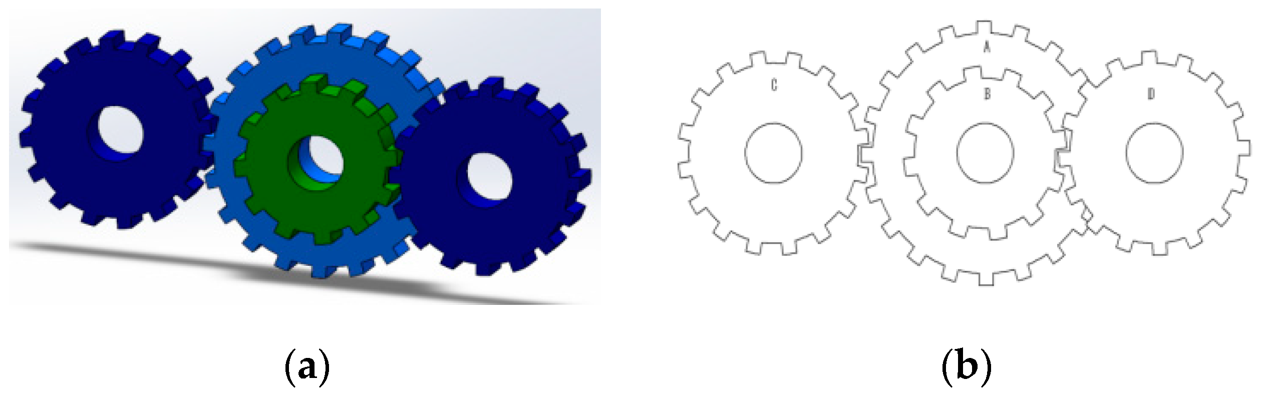
5.6. Gear Train Design Problem

The problem of gear train design is a classic engineering design problem. The gear train design problem is proposed to minimize the gear ratio. Within the benchmark suite, the problem features D = 4 decision variables, g = 2 inequality constraints, and h = 0 equality constraints. The optimal value of the objective function is known to be f (x*) = 0 [43]. Figure 15 illustrates the gear train configuration.
The design problem for the gear train can be outlined as follows:
Consider
x = [ x 1   x 2   x 3   x 4 ] = [ n A   n B   n C   n D ]
Objective function:
f ( x ) = 1 6.931 x 3 x 2 x 1 x 4 2
Subject to
g 1 ( x ) = 27 x 1 x 2 2 x 3 1 0
g 2 ( x ) = 397.5 x 1 x 2 2 x 3 2 1 0
Boundaries:
12 x 1 60
12 x 2 60
12 x 3 60
12 x 4 60
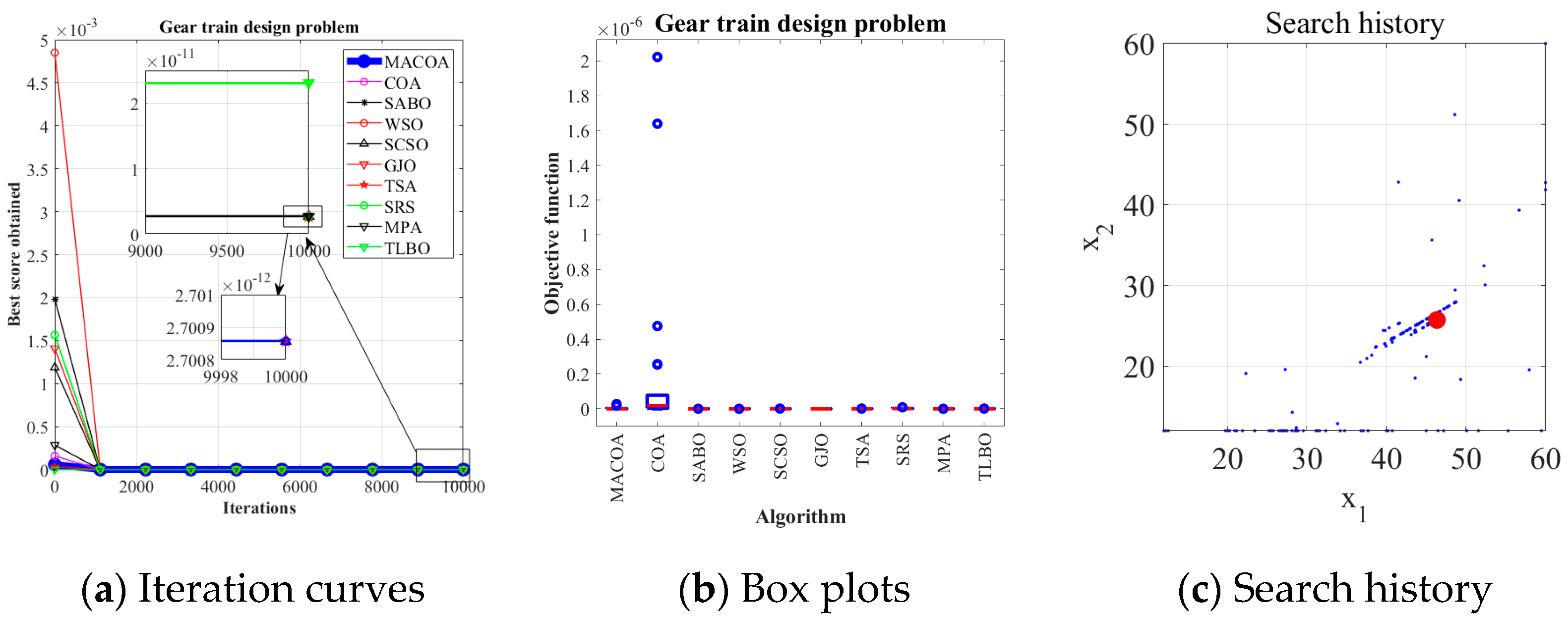
Table 15 shows that the SR of MACOA is 92%, which greatly exceeds that of COA. Figure 16a and Figure 16b show the iterative process and the box plot distribution of the optimal solutions for all the algorithms, respectively. Figure 16c shows the search history of MACOA over 10,000 iterations, with most of the search regions located in the region where the global optimum is located. These results further highlight the improved performance of MACOA compared to COA.

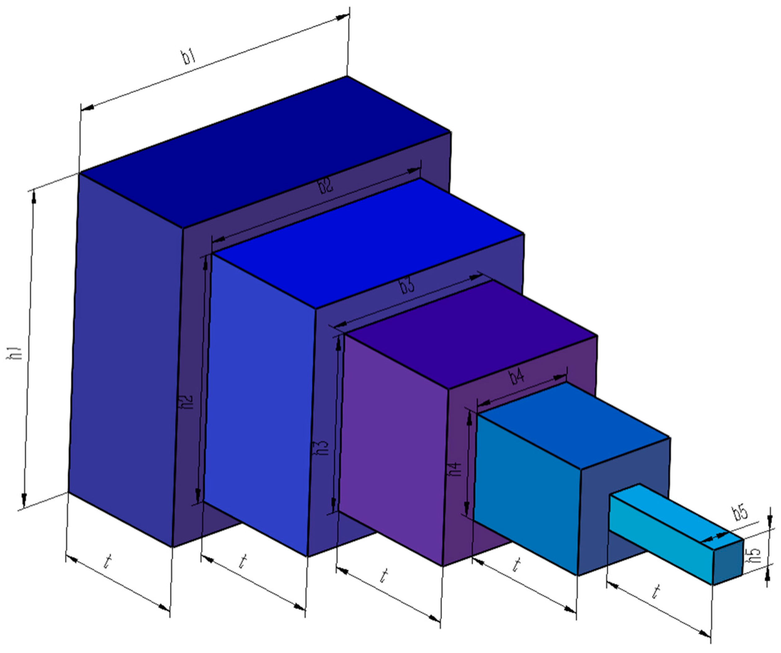
5.7. Cantilever Beam Design Problem

The design of a cantilever beam is a classic engineering design problem. Within the benchmark suite, the problem features D = 5 decision variables, g = 1 inequality constraints, and h = 0 equality constraints. The established optimal objective function f (x*) is 1.34 [43]. Figure 17 illustrates the cantilever beam configuration.
The design problem for the cantilever beam can be outlined as follows:
Consider
X = [ x 1   x 2   x 3   x 4   x 5 ]
Objective function:
f ( X ) = 0.0624   x 1 + x 2 + x 3 + x 4 + x 5
Subject to
g 1 ( X ) = 61 x 1 3 + 37 x 2 3 + 19 x 3 3 + 7 x 4 3 + 1 x 5 3 1 0
Boundaries:
0.01 x 1 100
0.01 x 2 100
0.01 x 3 100
0.01 x 4 100
0.01 x 5 100
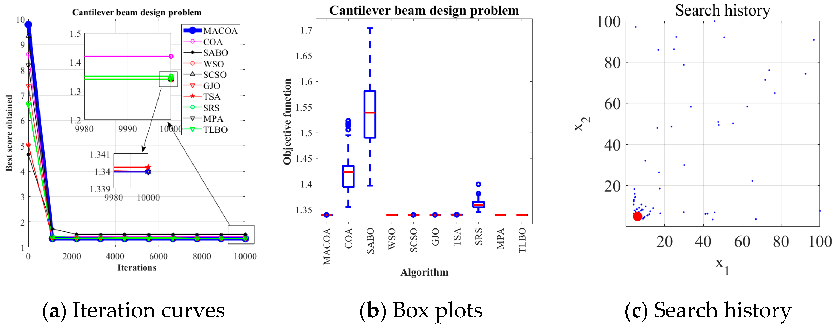
Table 16 shows that MACOA has both FR and SR of 100. These metrics far exceed COA and are comparable to the performance of WSO, SCSO, MPA, and TLBO. Figure 18a shows the iterative convergence process of all the algorithms. Figure 18b shows the boxplot distribution, from which it can be seen that MACOA has better stability and convergence than COA. Figure 18c shows the search history of MACOA, where most of the searches are clustered around the global optimum. MACOA also demonstrates better population convergence. These results show that MACOA’s performance is very competitive, not only outperforming COA, but also being on par with other good optimization algorithms.

5.8. Summary of Engineering Problems

Examining the data gathered from tackling the seven engineering problems discussed above, it is clear that the MACOA algorithm excels compared to other algorithms regarding feasibility and success rate in most engineering problems. This demonstrates MACOA’s exceptional capability to solve constrained engineering problems.

6. Conclusions and Future Prospects

The challenge of slow convergence and the tendency of COA to converge to local optima are addressed in this paper. To mitigate these issues, MACOA is introduced, which integrates Lévy flight, nonlinear inertia weight factors, and the coati vigilante mechanism. The Lévy flight mechanism is introduced into the population initialization phase to improve the quality of initial solutions. Then, the nonlinear inertia weight factors are introduced in the exploration phase to improve COA’s global search capabilities and accelerate convergence. Additionally, the coati vigilante mechanism is implemented in the exploitation phase to enable the algorithm to quickly escape from local optima and address the imbalance between the exploration and exploitation capabilities of COA.
Experiments are conducted based on the IEEE CEC2017 test functions, comparing MACOA with 11 other popular algorithms across three dimensions. The analysis of convergence curves, boxplots, and search history results indicates that MACOA achieves the best performance on 9 test functions with an average ranking of 2.17 in the 30-dimensional experiment, 12 test functions with an average ranking of 1.90 in the 50-dimensional experiment, and 14 test functions with an average ranking of 1.76 in the 100-dimensional experiment. Overall, MACOA outperforms all compared algorithms in the CEC2017 test function experiments.
In application experiments, MACOA is tested on seven engineering problems. By analyzing the experimental results, it is clear that MACOA exhibits the best performance in four of these problems and outperforms COA in all application scenarios. Therefore, the proposed MACOA significantly improves the performance of COA and holds strong application value in constrained engineering optimization problems.
Although MACOA is overall effective at present, there are still some areas that need further improvement. In the standard test function experiments, MACOA did not perform well on some functions compared to other algorithms. In future work, we will continue our research on several optimization strategies, particularly the nonlinear strategy in this study, where the adaptive parameters change with iterations. In addition, we are working on the challenges of its integration with other complex disciplinary issues. These efforts will further validate the adaptability and effectiveness of MACOA in different domains.

Author Contributions

Conceptualization, X.W. and Y.D.; methodology, X.W. and H.Z.; software, X.W.; validation, Y.D. and L.W.; formal analysis, X.W. and Y.D.; investigation, Y.D. and H.Z.; data curation, X.W.; writing—original draft preparation, X.W.; writing—review and editing, Y.D.; visualization, X.W.; supervision, Y.D.; project administration, Y.D.; funding acquisition, L.W. All authors have read and agreed to the published version of the manuscript.

Funding

This research was funded by the Shanghai Science and Technology Innovation Action Plan, grant number 23J21900100.

Institutional Review Board Statement

Not applicable.

Informed Consent Statement

Not applicable.

Data Availability Statement

The data generated from the analysis in this study can be found in this article. Any additional information required to reanalyze the data reported in this paper is available from the lead contact upon request.

Conflicts of Interest

Author Lin Wang was employed by the company Amerson Biomedical (Shanghai) Co., Ltd. The remaining authors declare that the research was conducted in the absence of any commercial or financial relationships that could be construed as a potential conflict of interest.

References

  1. Tan, J.; Melkoumian, N.; Harvey, D.; Akmeliawati, R. Nature-Inspired Solutions for Sustainable Mining: Applications of NIAs, Swarm Robotics, and Other Biomimicry-Based Technologies. Biomimetics 2025, 10, 181. [Google Scholar] [CrossRef] [PubMed]
  2. Xu, M.; Cao, L.; Lu, D.; Hu, Z.; Yue, Y. Application of swarm intelligence optimization algorithms in image processing: A comprehensive review of analysis, synthesis, and optimization. Biomimetics 2023, 8, 235. [Google Scholar] [CrossRef] [PubMed]
  3. Wu, W.; Li, B.; Chen, L.; Gao, J.; Zhang, C. A review for weighted minhash algorithms. IEEE Trans. Knowl. Data Eng. 2020, 34, 2553–2573. [Google Scholar] [CrossRef]
  4. Varshney, M.; Kumar, P.; Ali, M.; Gulzar, Y. Using the Grey Wolf Aquila Synergistic Algorithm for Design Problems in Structural Engineering. Biomimetics 2024, 9, 54. [Google Scholar] [CrossRef]
  5. Dehghani, M.; Montazeri, Z.; Trojovská, E.; Trojovský, P. Coati Optimization Algorithm: A new bio-inspired metaheuristic algorithm for solving optimization problems. Knowl. Based Syst. 2023, 259, 110011. [Google Scholar] [CrossRef]
  6. Wu, D.; Xie, Y.; Qiang, Z. An efficient EM algorithm for two-layer mixture model of gaussian process functional regressions. Pattern Recognit. 2023, 143, 109783. [Google Scholar] [CrossRef]
  7. Wolpert, D.H.; Macready, W.G. No free lunch theorems for optimization. IEEE Trans. Evol. Comput. 1997, 1, 67–82. [Google Scholar] [CrossRef]
  8. Kuyu, Y.Ç.; Vatansever, F. Advanced metaheuristic algorithms on solving multimodal functions: Experimental analyses and performance evaluations. Arch. Comput. Methods Eng. 2021, 28, 4861–4873. [Google Scholar] [CrossRef]
  9. Yan, Y.; Zhu, Y.; Liu, R.; Zhang, Y.; Zhang, Y.; Zhang, L. Spatial distribution-based imbalanced undersampling. IEEE Trans. Knowl. Data Eng. 2022, 35, 6376–6391. [Google Scholar] [CrossRef]
  10. Shang, S.; Zhu, J.; Liu, Q.; Shi, Y.; Qiao, T. Low-altitude small target detection in sea clutter background based on improved CEEMDAN-IZOA-ELM. Heliyon 2024, 10, e26500. [Google Scholar] [CrossRef]
  11. Wang, C.; Yang, G.; Li, J.; Huang, Q. Fuzzy adaptive PSO-ELM algorithm applied to vehicle sound quality prediction. Appl. Sci. 2023, 13, 9561. [Google Scholar] [CrossRef]
  12. Zhang, Y.; Mo, Y. Chaotic adaptive sailfish optimizer with genetic characteristics for global optimization. J. Supercomput. 2022, 78, 10950–10996. [Google Scholar] [CrossRef]
  13. Hassan, M.H.; Kamel, S.; Mohamed, A.W. Enhanced gorilla troops optimizer powered by marine predator algorithm: Global optimization and engineering design. Sci. Rep. 2024, 14, 7650. [Google Scholar] [CrossRef] [PubMed]
  14. Zhu, M.; Zhu, R.; Li, F.; Qiu, J. An improved slime mould algorithm using multiple strategies. Int. J. Parallel Emergent Distrib. Syst. 2024, 39, 461–485. [Google Scholar] [CrossRef]
  15. Yan, Y.; Qian, Y.; Ma, H.; Hu, C. Research on imbalanced data fault diagnosis of on-load tap changers based on IGWO-WELM. Math. Biosci. Eng 2023, 20, 4877–4895. [Google Scholar] [CrossRef]
  16. Gürses, D.; Bureerat, S.; Sait, S.M.; Yıldız, A.R. Comparison of the arithmetic optimization algorithm, the slime mold optimization algorithm, the marine predators algorithm, the salp swarm algorithm for real-world engineering applications. Mater. Test. 2021, 63, 448–452. [Google Scholar] [CrossRef]
  17. Dehghani, M.; Montazeri, Z.; Dhiman, G.; Malik, O.P.; Morales-Menendez, R.; Ramirez-Mendoza, R.A.; Dehghani, A.; Guerrero, J.M.; Parra-Arroyo, L. A spring search algorithm applied to engineering optimization problems. Appl. Sci. 2020, 10, 6173. [Google Scholar] [CrossRef]
  18. Jia, H.; Shi, S.; Wu, D.; Rao, H.; Zhang, J.; Abualigah, L. Improve coati optimization algorithm for solving constrained engineering optimization problems. J. Comput. Des. Eng. 2023, 10, 2223–2250. [Google Scholar] [CrossRef]
  19. Qi, Z.; Yingjie, D.; Shan, Y.; Xu, L.; Dongcheng, H.; Guoqi, X. An improved Coati Optimization Algorithm with multiple strategies for engineering design optimization problems. Sci. Rep. 2024, 14, 20435. [Google Scholar] [CrossRef]
  20. Başak, H. Hybrid coati–grey wolf optimization with application to tuning linear quadratic regulator controller of active suspension systems. Eng. Sci. Technol. Int. J. 2024, 56, 101765. [Google Scholar] [CrossRef]
  21. Baş, E.; Yildizdan, G. Enhanced coati optimization algorithm for big data optimization problem. Neural Process. Lett. 2023, 55, 10131–10199. [Google Scholar] [CrossRef]
  22. Wang, C.; Lin, H.; Yang, M.; Fu, X.; Yuan, Y.; Wang, Z. A novel chaotic time series wind power point and interval prediction method based on data denoising strategy and improved coati optimization algorithm. Chaos Solitons Fractals 2024, 187, 115442. [Google Scholar] [CrossRef]
  23. Mu, G.; Li, J.; Liu, Z.; Dai, J.; Qu, J.; Li, X. MSBKA: A Multi-Strategy Improved Black-Winged Kite Algorithm for Feature Selection of Natural Disaster Tweets Classification. Biomimetics 2025, 10, 41. [Google Scholar] [CrossRef]
  24. Zhou, Y.; Hao, Z. Multi-Strategy Improved Whale Optimization Algorithm and Its Engineering Applications. Biomimetics 2025, 10, 47. [Google Scholar] [CrossRef] [PubMed]
  25. Meng, W.; He, Y.; Zhou, Y. Q-Learning-Driven Butterfly Optimization Algorithm for Green Vehicle Routing Problem Considering Customer Preference. Biomimetics 2025, 10, 57. [Google Scholar] [CrossRef]
  26. Oueslati, R.; Manita, G.; Chhabra, A.; Korbaa, O. Chaos game optimization: A comprehensive study of its variants, applications, and future directions. Comput. Sci. Rev. 2024, 53, 100647. [Google Scholar] [CrossRef]
  27. Akgul, A.; Karaca, Y.; Pala, M.A.; Çimen, M.E.; Boz, A.F.; Yildiz, M.Z. Chaos theory, advanced metaheuristic algorithms and their newfangled deep learning architecture optimization applications: A review. Fractals 2024, 32, 2430001. [Google Scholar] [CrossRef]
  28. Chawla, M.; Duhan, M. Levy flights in metaheuristics optimization algorithms—A review. Appl. Artif. Intell. 2018, 32, 802–821. [Google Scholar] [CrossRef]
  29. Xue, J.; Shen, B. A novel swarm intelligence optimization approach: Sparrow search algorithm. Syst. Sci. Control Eng. 2020, 8, 22–34. [Google Scholar] [CrossRef]
  30. Das, S.; Suganthan, P.N. Differential evolution: A survey of the state-of-the-art. IEEE Trans. Evol. Comput. 2010, 15, 4–31. [Google Scholar] [CrossRef]
  31. Wu, G.; Mallipeddi, R.; Suganthan, P.N. Problem Definitions and Evaluation Criteria for the CEC 2017 Competition on Constrained Real-Parameter Optimization; Technical Report; National University of Defense Technology: Changsha, China; Kyungpook National University: Daegu, Republic of Korea; Nanyang Technological University: Singapore, 2017. [Google Scholar]
  32. Trojovský, P.; Dehghani, M. Subtraction-average-based optimizer: A new swarm-inspired metaheuristic algorithm for solving optimization problems. Biomimetics 2023, 8, 149. [Google Scholar] [CrossRef] [PubMed]
  33. Braik, M.; Hammouri, A.; Atwan, J.; Al-Betar, M.A.; Awadallah, M.A. White Shark Optimizer: A novel bio-inspired meta-heuristic algorithm for global optimization problems. Knowl. Based Syst. 2022, 243, 108457. [Google Scholar] [CrossRef]
  34. Seyyedabbasi, A.; Kiani, F. Sand Cat swarm optimization: A nature-inspired algorithm to solve global optimization problems. Eng. Comput. 2023, 39, 2627–2651. [Google Scholar] [CrossRef]
  35. Chopra, N.; Ansari, M.M. Golden jackal optimization: A novel nature-inspired optimizer for engineering applications. Expert Syst. Appl. 2022, 198, 116924. [Google Scholar] [CrossRef]
  36. Kaur, S.; Awasthi, L.K.; Sangal, A.; Dhiman, G. Tunicate Swarm Algorithm: A new bio-inspired based metaheuristic paradigm for global optimization. Eng. Appl. Artif. Intell. 2020, 90, 103541. [Google Scholar] [CrossRef]
  37. Mirjalili, S.; Lewis, A. The whale optimization algorithm. Adv. Eng. Softw. 2016, 95, 51–67. [Google Scholar] [CrossRef]
  38. Mirjalili, S.; Mirjalili, S.M.; Lewis, A. Grey wolf optimizer. Adv. Eng. Softw. 2014, 69, 46–61. [Google Scholar] [CrossRef]
  39. Rao, R.; Savsani, V.; Vakharia, D. Teaching–learning-based optimization: An optimization method for continuous non-linear large scale problems. Inf. Sci. 2012, 183, 1–15. [Google Scholar] [CrossRef]
  40. Rashedi, E.; Nezamabadi-Pour, H.; Saryazdi, S. GSA: A gravitational search algorithm. Inf. Sci. 2009, 179, 2232–2248. [Google Scholar] [CrossRef]
  41. Kennedy, J.; Eberhart, R. Particle swarm optimization. In Proceedings of the ICNN’95-International Conference on Neural Networks, Perth, WA, Australia, 27 November–1 December 1995; IEEE: Piscataway, NJ, USA, 1995; Volume 4. [Google Scholar]
  42. Price, K.V.; Kumar, A.; Suganthan, P.N. Trial-based dominance enables non-parametric tests to compare both the speed and accuracy of stochastic optimizers. arXiv 2022, arXiv:2212.09423. [Google Scholar]
  43. Kumar, A.; Wu, G.; Ali, M.Z.; Mallipeddi, R.; Suganthan, P.N.; Das, S. A test-suite of non-convex constrained optimization problems from the real-world and some baseline results. Swarm Evol. Comput. 2020, 56, 100693. [Google Scholar] [CrossRef]
  44. Goodarzimehr, V.; Shojaee, S.; Hamzehei-Javaran, S.; Talatahari, S. Special relativity search: A novel metaheuristic method based on special relativity physics. Knowl. Based Syst. 2022, 257, 109484. [Google Scholar] [CrossRef]
  45. Faramarzi, A.; Heidarinejad, M.; Mirjalili, S.; Gandomi, A.H. Marine Predators Algorithm: A nature-inspired metaheuristic. Expert Syst. Appl. 2020, 152, 113377. [Google Scholar] [CrossRef]
Figure 1. Flowchart of the MACOA.
Biomimetics 10 00323 g001
Figure 2. Box plots comparing MACOA and the other 11 algorithms based on the CEC-2017 (dimension m = 50).
Biomimetics 10 00323 g002aBiomimetics 10 00323 g002b
Figure 3. Iteration curves and search history of the proposed MACOA and the other 11 algorithms based on CEC2017 (dimension m = 30).
Biomimetics 10 00323 g003aBiomimetics 10 00323 g003bBiomimetics 10 00323 g003cBiomimetics 10 00323 g003dBiomimetics 10 00323 g003eBiomimetics 10 00323 g003f
Figure 4. Iteration curves of MACOA and the compared algorithms based on the CEC-2017 (dimension m = 100).
Biomimetics 10 00323 g004aBiomimetics 10 00323 g004b
Figure 5. (a) Model diagram of the three-bar truss design problem. (b) Schematic of the three-bar truss design problem.
Biomimetics 10 00323 g005
Figure 6. Iteration curves and box plots of the ten algorithms applied to the three-bar truss design problem.
Biomimetics 10 00323 g006
Figure 7. Schematic of the tension or compression spring design problem.
Biomimetics 10 00323 g007
Figure 8. Iteration curves and box plots of the algorithms applied to the tension or compression spring design problem.
Biomimetics 10 00323 g008
Figure 9. (a) Model diagram of the pressure vessel design problem. (b) Schematic of the pressure vessel design problem.
Biomimetics 10 00323 g009
Figure 10. Iteration curves and boxplots of the ten algorithms applied to the pressure vessel design problem.
Biomimetics 10 00323 g010
Figure 11. (a) Model diagram of the welded beam design problem. (b) Schematic of the welded beam design problem.
Biomimetics 10 00323 g011
Figure 12. Convergence curves and box plots of the ten algorithms applied to the welded beam design problem.
Biomimetics 10 00323 g012
Figure 13. (a) Model diagram of the speed reducer design problem. (b) Schematic of the speed reducer design problem.
Biomimetics 10 00323 g013
Figure 14. Iteration curves and box plots of the ten algorithms applied to the speed reducer design problem.
Biomimetics 10 00323 g014
Figure 15. (a) Model diagram of the gear train design problem. (b) Schematic of the gear train design problem.
Biomimetics 10 00323 g015
Figure 16. Iteration curves and boxplots of MACOA and the other algorithms for the gear train design problem.
Biomimetics 10 00323 g016
Figure 17. Schematic of the cantilever beam design problem.
Biomimetics 10 00323 g017
Figure 18. Iteration curves and box plots of the ten algorithms applied to the cantilever beam design problem.
Biomimetics 10 00323 g018
Table 1. Pseudo-code of MACOA.
Start MACOA.
Input the optimization problem information.
   Set the number of iterations T and the number of coatis N.
  Initialization of coatis and evaluation of the objective function for the population using (7)–(9).
For t = 1:T
   Update location of the iguana based on the location of the best member of the population.
   Phase 1: Exploration Phase
   Calculate the weighted factor ω using (10)
   For i = 1:[N/2]
    Calculate new position for the i-th coati by (11).
    Update position of the i-th coati using (4).
   End for
   for i = N/2 +1:N
Calculate random position for the iguana using (2).
Calculate new position for the i-th coati using (3).
Update position of the i-th coati using (4).
   End for
   Phase 2: Exploitation Phase
   For i = 1:N
      Calculate the new position for the i-th coati using (13).
      Update the position of the i-th coati using (4).
   End for
   Save the best candidate solution found so far
End for
Output of the best obtained solution by MACOA for given problem.
End MACOA.
Table 2. Control parameter values for the algorithms being compared.
Alg.ParameterValueAlg.ParameterValue
COAr: random number[0, 1]WOAa: Convergence parameterLinear reduction from 2 to 0.
I: random number{0, 1}r: random vector[0, 1]
SABOv: random vector[1, 2]l: random number[−1, 1]
ri: random numberri obeys a normal distributionGWOConvergence parameter (a)Linear reduction from 2 to 0.
WSOfmin0.07TLBOTF: teaching factorTF = round [(1 + rand)]
fmax0.75Random number[0, 1]
τ4.11GSAAlpha20
a06.25Rpower1
a1100Rnorm2
a20.0005G0100
SCSOrGLinear reduction from 2 to 0.PSOTopologyFully connected.
SM2Cognitive constantC1 = 2
GJOc11.5Social constantC2 = 2
E0: random number[−1, 1]Inertia weightLinear reduction from 0.9 to 0.1.
β1.5Velocity limit10% of the dimensions range of the variables.
TSAPmin1WOAa: Convergence parametera: Linear reduction from 2 to 0.
Pmax4r: random vector[0, 1]
c1, c2, c3Random in [0, 1]l: random number[−1, 1]
Table 3. Time complexity comparison between MACOA and the other 11 algorithms based on the CEC-2017.
MACOACOASABOWSOSCSOGJOTSAWOAGWOTLBOGSAPSO
F1852.5946879.1897509.3283444.06387430.23721488.9901981.1678440.2204951.00891595.08241734.3884894.0729
F31020.66221022.7472727.0783551.57467199.44531278.7816863.0205350.4119845.62341071.40261526.6804770.3774
F4932.7085920.0671658.0728608.89707041.94311156.2279829.5889388.62701055.04481044.78611512.6196772.6830
F51310.38271349.9389977.0681635.24197280.42221490.59981017.1022578.96481114.76161584.56911668.74741205.1916
F63206.21873257.66661656.91261440.94068821.85102411.97271890.82041322.99371811.54453770.28102663.45952713.9477
F71372.05391288.7758782.7713663.46406866.76191437.78431011.0877609.09901131.49851736.48511683.86581105.1710
F81705.47951618.2586989.0674758.64538018.23171703.77621208.4044707.09911179.30741791.31021850.40341349.2233
F91648.60601651.05341003.9989787.21437871.86311683.26071213.8018706.45271227.06541776.20221956.89151337.1876
F102006.97591924.22301087.8128844.96147858.71541727.07461286.4960774.88431269.48782099.03462061.40721556.3573
F111429.52881345.2243886.8715648.10527671.36741591.87281076.9965568.02701047.31301996.22381802.46071151.6052
F121707.72021715.73951056.6301746.11668187.43041783.05181249.7590738.47981189.73212169.57812011.43511447.6008
F131374.97311392.5722916.9523604.33277316.27021569.6265964.5263527.21791048.76101713.44241966.85511244.0637
F141495.80661510.9372813.7888630.37736341.59621057.0906998.5398584.80961055.08321223.21361551.76611311.9379
F15920.7320829.8522539.6170473.16576433.94941043.8119831.0791400.1807886.7541997.80841593.65381014.5658
F161377.20761422.0340777.4971601.31607099.01531383.3329847.1459500.7935969.47621119.95811501.59041134.0044
F172240.51262367.80511179.4587933.64987030.90061617.45421273.5408856.29201363.39211960.52061786.77911711.5786
F181312.71821286.5012762.6733508.72106978.99891253.0395923.6291499.25801065.15391305.96131549.29261123.3055
F199161.54009250.56304060.23243705.024411,388.70784957.64484174.81653806.55684324.00798694.88135438.81937863.7214
F202315.37042213.69331065.6800943.95586971.19511875.79162086.32671038.46591537.55002631.34542006.69122248.4016
F213899.95813845.71281697.27271524.91398402.96942783.35092117.37661609.15122042.75493562.70312991.91783465.8951
F224347.65174271.32481957.74701801.43338400.88352624.56532143.90291751.95752144.35263972.41133071.84353872.0125
F235243.38805095.28692343.78991945.22208023.09862870.12152572.97832019.18462638.23514842.50773447.06254812.5093
F245859.59715815.14032703.22622198.25379893.71073412.48702958.02992381.33812782.02505347.27453702.84565184.9546
F255234.08715325.21222328.71952169.16958902.07963287.35852627.79422089.52912537.60934462.62483028.22974218.4649
F266053.03986210.60522721.72912488.04998755.16733203.41362870.92272351.24272835.72355087.63323515.92235614.6762
F277363.31177377.85853176.24892678.65989494.82373698.53703358.67152957.47883373.35466099.72694054.02895826.5099
F286043.97956153.32062753.79412444.20128661.43583284.10572925.96652448.15542955.49365578.78063508.56144854.3631
F294402.08494255.11722049.28571816.38317972.26702373.50162140.26421814.00772068.33723796.20732672.30203387.8230
F3011,255.952111,151.53824794.73833477.028711,783.63975529.23515132.70994466.06944932.968710,230.82986440.095210,042.3783
Table 4. Space complexity comparison between MACOA and the other 11 algorithms.
Space Complexity Space Complexity
MACOAO(pop × dim)TSAO(pop × dim)
COAO(pop × dim)WOAO(pop × dim)
SABOO(pop × dim)GWOO(pop × dim)
WSOO(pop × dim + Max × dim)TLBOO(pop × dim)
SCSOO(pop × dim + Max)GSAO(Max × pop × dim)
GJOO(pop × dim)PSOO(pop × dim + Max)
Table 5. Summary of the CEC-2017 test functions.
NameNo.FunctionsFi (x*)No.FunctionsFi (x*)
Unimodal
Functions
1Shifted and Rotated Bent Cigar Function1003Shifted and Rotated Zakharov Function200
Simple
Multimodal Functions
4Shifted and Rotated Rosenbrock’s Function3008Shifted and Rotated Non-Continuous Rastrigin’s Function700
5Shifted and Rotated Rastrigin’s Function400
6Shifted and Rotated Expanded Scaffer’s F6 Function5009Shifted and Rotated Levy Function800
7Shifted and Rotated Lunacek Bi_Rastrigin Function60010Shifted and Rotated Schwefel’s Function900
Hybrid
Functions
11Hybrid Functions 1 (N = 3)100016Hybrid Functions 6 (N = 4)1500
12Hybrid Functions 2 (N = 3)110017Hybrid Functions 6 (N = 5)1600
13Hybrid Functions 3 (N = 3)120018Hybrid Functions 6 (N = 5)1700
14Hybrid Functions 4 (N = 4)130019Hybrid Functions 6 (N = 5)1800
15Hybrid Functions 5 (N = 4)140020Hybrid Functions 6 (N = 6)1900
Composition
Functions
21Composition Functions 1 (N = 3)200026Composition Functions 6 (N = 5)2500
22Composition Functions 2 (N = 3)210027Composition Functions 7 (N = 6)2600
23Composition Functions 3 (N = 4)220028Composition Functions 8 (N = 6)2700
24Composition Functions 4 (N = 4)230029Composition Functions 9 (N = 3)2800
25Composition Functions 5 (N = 5)240030Composition Functions 10 (N = 3)2900
Search Range: [−100, 100] dim
Table 6. Rank results comparing MACOA and the other 11 algorithms based on the CEC-2017 (the dimension m = 30).
MACOACOASABOWSOSCSOGJOTSAWOAGWOTLBOGSAPSO
F1211756891241310
F3210475861231119
F4111875691243210
F5211736491218510
F6210746381111259
F7211765491218310
F8310726591211148
F9410796511121238
F10110945671131228
F11111835791242610
F12211675891241310
F13312657810114129
F14311945710126281
F15411718910126235
F16311915481226710
F17512914281136710
F18211938610127451
F19311728910125146
F20310815461229711
F21296453811112710
F22111475691223810
F23286543710191112
F24111584379212610
F25111754681239210
F26111865391224710
F27311786592410121
F28112976811351042
F29111935461228710
F30211736810125149
Sum rank6331120913116016225131989170158239
Mean rank2.17210.7247.2074.5175.5175.5868.655113.0695.8625.4488.241
Total rank111835610122749
Table 7. Rank results comparing MACOA and the other 11 algorithms based on the CEC-2017 (the dimension m = 50).
MACOACOASABOWSOSCSOGJOTSAWOAGWOTLBOGSAPSO
F1111685791242310
F3611941321258107
F4111785691242310
F5211846510121739
F6297463101111258
F7211675391218410
F8211846510121739
F9310894611122517
F10110945671131228
F11111536781242910
F12212685791141310
F13212685791141310
F14212875610114193
F15211576810124139
F16112847691125310
F17211836491217510
F18111946810125237
F19312745810116129
F20310915471221168
F21210745381211169
F22198356711212410
F23110654379281112
F24112583461129710
F25111865791242310
F26111754391228610
F27311786591410122
F28312118791025461
F29111936481225710
F30211856791241310
Sum rank5531721515615016025031586165145248
Mean rank1.89710.9317.4145.3795.1725.5178.62110.8622.9665.69058.552
Total rank112854610112739
Table 8. Rank results comparing MACOA and the other 11 algorithms based on the CEC-2017 (the dimension m = 100).
MACOACOASABOWSOSCSOGJOTSAWOAGWOTLBOGSAPSO
F1111684951232710
F3564317101291182
F4111784561232910
F5210846511121739
F6298465101111237
F7211685391217410
F8211846510121739
F9297835111241016
F10110945671131228
F11411962731251810
F12111574691232810
F13211684791231510
F14111963871242510
F15211586791231410
F16111946581223710
F17111674591232810
F18211965781241310
F19211674891231510
F20210914671231158
F21210954361117812
F22110935671141228
F23111754389261210
F24112863471025119
F25111794861232510
F26111954361228710
F27312810569247111
F28312911687254101
F29111754681232910
F30111574691232810
Sum rank5130821417712516923031988150181250
Mean rank1.75910.6217.3796.1034.3105.8287.931113.0345.1726.2418.621
Total rank111863591224710
Table 9. Rank results of the ablation experiment for MACOA with CEC-2017 (dimension = 10).
COACOA + LCOA + NCOA + VCOA + L + NCOA + L + VCOA + N + VMACOA
F187536142
F378516111
F487615423
F578562341
F687635241
F787546213
F878231564
F987564321
F1087645132
F1187465213
F1287645321
F1378625413
F1475846132
F1578536412
F1687364152
F1778516342
F1858637412
F1986735412
F2078635214
F2176485111
F2287136524
F2387412635
F2458174622
F2587453216
F2678415631
F2778562341
F2878364215
F2987345261
F3078635412
Sum rank213212136110135877169
Mean rank7.3457.3104.6903.7934.65532.4482.379
Total rank87645321
Table 10. Comparative analysis of the three-bar truss design problem.
Alg.BestStdMeanMedianWorstFRSR
MACOA263.895840.00001263.89585263.89584263.89588210
COA263.896040.00742263.90185263.89927263.9299500
SABO263.899350.02207263.92659263.92195264.0087700
WSO263.895870.00000263.89587263.89587263.8958700
SCSO263.895850.00012263.89592263.89588263.8966200
GJO263.895900.00052263.89647263.89634263.8984200
TSA263.895930.00111263.89761263.89757263.9012500
SRS263.898862.04942264.70462263.97716270.9139400
MPA263.895840.00001263.89585263.89584263.89587818
TLBO263.895840.00000263.89584263.89584263.89584070
Table 11. Comparative analysis of the tension or compression spring design problem.
Alg.BestStdMeanMedianWorstFRSR
MACOA0.0126120.0009970.0128630.0126650.0176989898
COA0.0126870.0025290.0134880.0130320.03045500
SABO0.0126800.0001560.0128010.0127400.01354200
WSO0.0126650.0000000.0126650.0126650.0126650100
SCSO0.0126650.0000420.0127080.0127030.01284302
GJO0.0126670.0000200.0126920.0126870.01272200
TSA0.0126700.0000150.0126950.0126920.01273800
SRS0.0127100.0001100.0129090.0128850.01310800
MPA0.0126650.0000000.0126650.0126650.0126650100
TLBO0.0126650.0000010.0126660.0126660.012670016
Table 12. Results of the pressure vessel design problem experiments.
Alg.BestStdMeanMedianWorstFRSR
MACOA5.885 × 1036.122 × 1026.335 × 1035.934 × 1037.319 × 1031616
COA7.141 × 1034.428 × 1046.047 × 1045.226 × 1042.036 × 10500
SABO6.379 × 1034.770 × 1027.134 × 1037.036 × 1038.499 × 10300
WSO5.885 × 1039.187 × 10−135.885 × 1035.885 × 1035.885 × 10300
SCSO5.885 × 1035.175 × 1026.327 × 1036.023 × 1037.319 × 10300
GJO5.886 × 1034.3525.889 × 1035.889 × 1035.915 × 10300
TSA5.889 × 1031.169 × 1025.931 × 1035.910 × 1036.716 × 10300
SRS5.989 × 1031.741 × 1026.312 × 1036.335 × 1036.804 × 10300
MPA5.885 × 1039.187 × 10−135.885 × 1035.885 × 1035.885 × 1030100
TLBO5.885 × 1032.282 × 10−85.885 × 1035.885 × 1035.885 × 103098
Table 13. Experimental results of the welded beam design problem.
Alg.BestStdMeanMedianWorstFRSR
MACOA1.6623.351 × 10−21.6771.6621.7538484
COA1.7352.118 × 10−12.4272.4882.77300
SABO1.6915.034 × 10−11.9811.7853.50200
WSO1.6620.0001.6621.6621.662100100
SCSO1.6622.402 × 10−41.6621.6621.663100100
GJO1.6624.905 × 10−41.6631.6631.665100100
TSA1.6661.737 × 10−31.6701.6701.6744848
SRS1.7042.433 × 10−21.7541.7561.82700
MPA1.6622.243 × 10−161.6621.6621.662100100
TLBO1.6622.243 × 10−161.6621.6621.662100100
Table 14. Experimental results of the speed reducer design problem.
Alg.BestStdMeanMedianWorstFRSR
MACOA2.994 × 1032.679 × 1013.010 × 1033.006 × 1033.164 × 1034646
COA3.029 × 1034.527 × 10971.058 × 10973.281 × 1032.282 × 109800
SABO3.220 × 1034.607 × 1024.360 × 1034.343 × 1035.277 × 10300
WSO2.994 × 1030.0002.994 × 1032.994 × 1032.994 × 103100100
SCSO2.995 × 1034.0753.000 × 1033.001 × 1033.010 × 10300
GJO2.995 × 1034.4213.002 × 1033.001 × 1033.013 × 10300
TSA3.006 × 1035.3363.018 × 1033.019 × 1033.032 × 10300
SRS3.041 × 1032.395 × 1013.081 × 1033.076 × 1033.149 × 10300
MPA2.994 × 1030.0002.994 × 1032.994 × 1032.994 × 103100100
TLBO2.994 × 1036.496 × 10−142.994 × 1032.994 × 1032.994 × 103100100
Table 15. Experimental results of the gear train design problem.
Alg.BestStdMeanMedianWorstFRSR
MACOA2.7009 × 10−126.8154 × 10−92.4924 × 10−98.8876 × 10−102.7265 × 10−8092
COA2.7009 × 10−124.5433 × 10−71.6367 × 10−71.8274 × 10−82.0226 × 10−6082
SABO2.7009 × 10−121.7358 × 10−118.2394 × 10−122.7009 × 10−121.1661 × 10−100100
WSO2.7009 × 10−126.1753 × 10−124.7386 × 10−122.7009 × 10−122.3078 × 10−110100
SCSO2.7009 × 10−124.2280 × 10−102.4751 × 10−102.3078 × 10−119.9216 × 10−100100
GJO2.7009 × 10−129.4329 × 10−128.8140 × 10−122.7009 × 10−122.3078 × 10−110100
TSA2.7009 × 10−123.2309 × 10−101.2633 × 10−102.7009 × 10−129.9216 × 10−100100
SRS2.7009 × 10−122.3366 × 10−92.1648 × 10−91.3616 × 10−98.7008 × 10−90100
MPA2.7009 × 10−122.8818 × 10−123.1084 × 10−122.7009 × 10−122.3078 × 10−110100
TLBO2.7009 × 10−121.3927 × 10−102.9418 × 10−112.7009 × 10−129.9216 × 10−100100
Table 16. Results of the cantilever beam design problem experiments.
Alg.BestStdMeanMedianWorstFRSR
MACOA1.339960.000001.339961.339961.33996100100
COA1.355350.044471.425511.423571.5235100
SABO1.397120.066721.541731.539021.7034000
WSO1.339960.000001.339961.339961.33996100100
SCSO1.339960.000001.339961.339961.33997100100
GJO1.339960.000011.339971.339971.340019898
TSA1.340030.000121.340341.340341.3407200
SRS1.345370.010401.360891.359301.3995700
MPA1.339960.000001.339961.339961.33996100100
TLBO1.339960.000001.339961.339961.33996100100
Disclaimer/Publisher’s Note: The statements, opinions and data contained in all publications are solely those of the individual author(s) and contributor(s) and not of MDPI and/or the editor(s). MDPI and/or the editor(s) disclaim responsibility for any injury to people or property resulting from any ideas, methods, instructions or products referred to in the content.

