


Application of Metaheuristics for Optimizing Predictive Models in iHealth: A Case Study on Hypotension Prediction in Dialysis Patients

 , , ,
, , ,  ,
,  , , , and
Abstract
1. Introduction
- Use a metaheuristic approach to solve the feature selection problem in the context of hemodialysis and apply two objective functions for this problem.
- Use four metaheuristic algorithms: Particle Swarm Optimization, Grey Wolf Optimizer, Pendulum Search Algorithm, and Whale Optimization Algorithm. In addition, use three classification algorithms, K-Nearest Neighbors, Random Forest, and XGBoost, to evaluate the efficiency of the metaheuristic algorithms.
- Perform in-depth analysis using various performance metrics such as recall, F-score, precision, and number of selected features, graphs, and statistical tests.
2. Background and Related Works
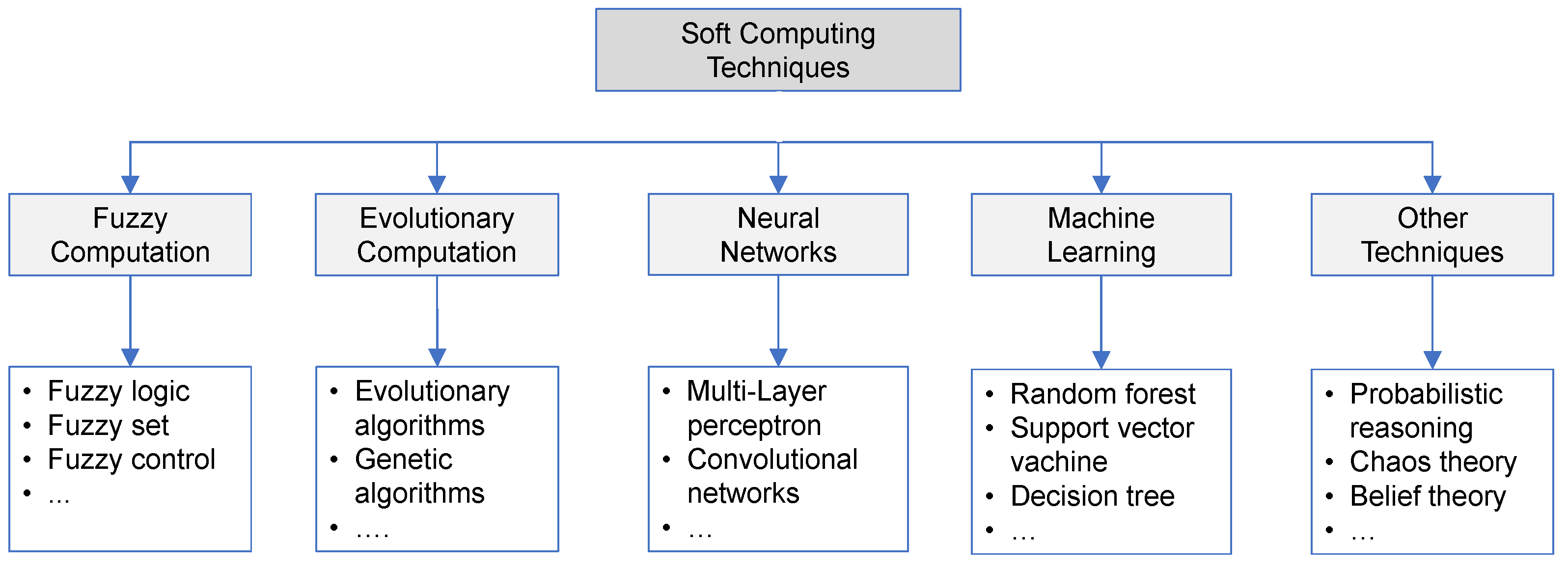
2.1. Soft Computing Techniques in Healthcare
2.2. Optimization Techniques for IDH Prediction
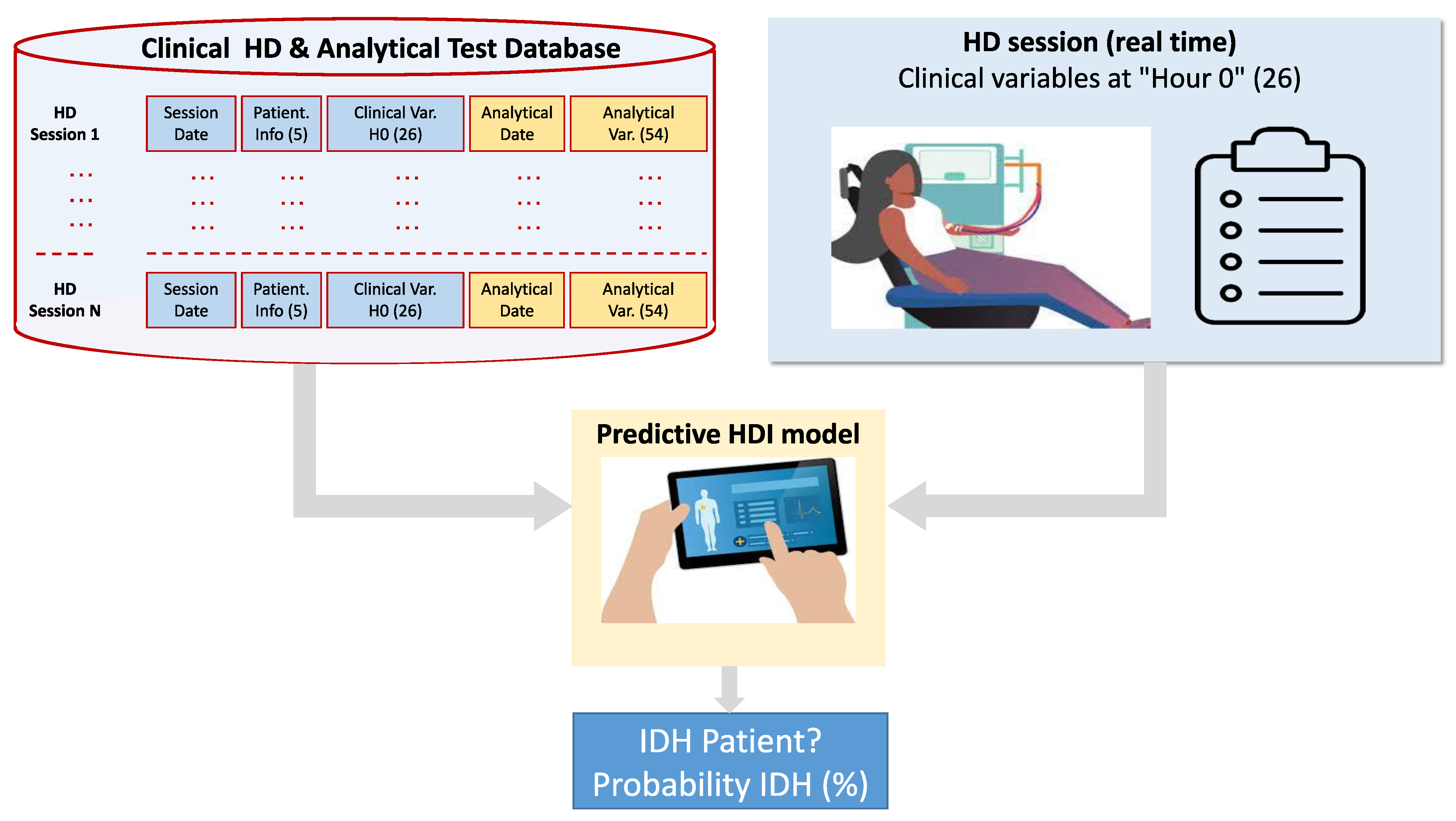
3. Hypotension Dataset
3.1. Digitized Clinical Database of Hemodialysis Patients
3.2. Determination of IDH in the HD Session
3.3. Data Processing and Variables Considered in the Clinical Study
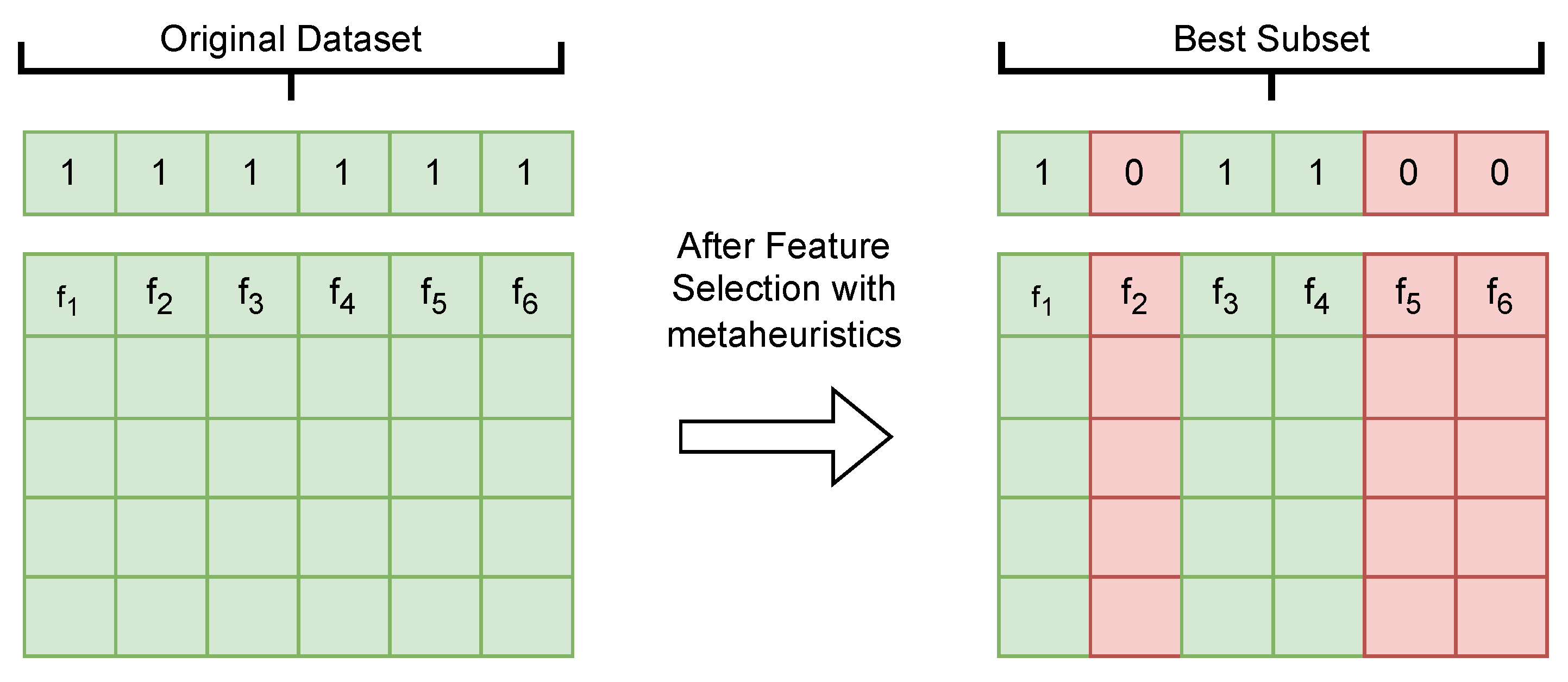
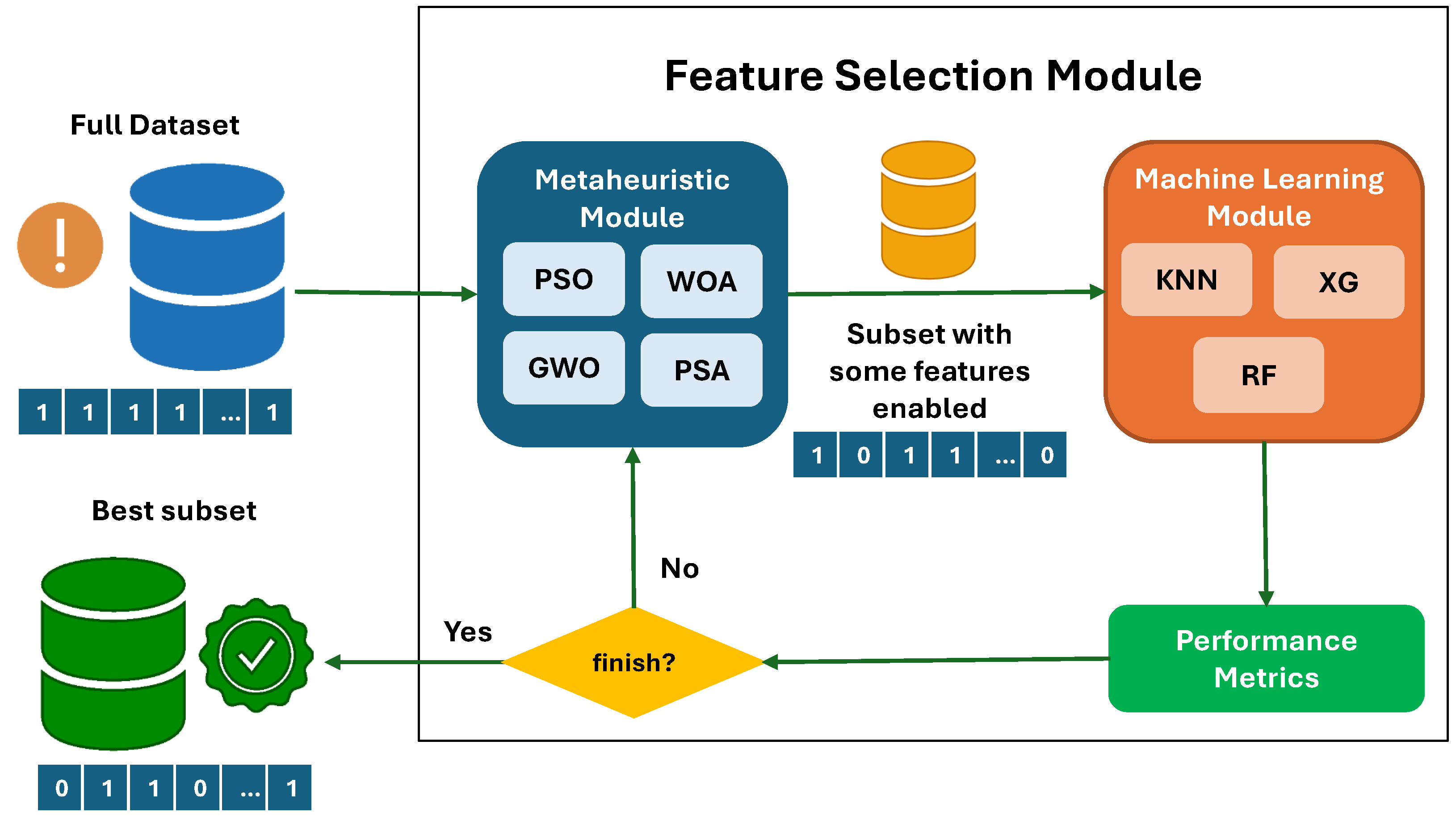
4. Optimization of Relevant Feature Selection for the Predictive Model
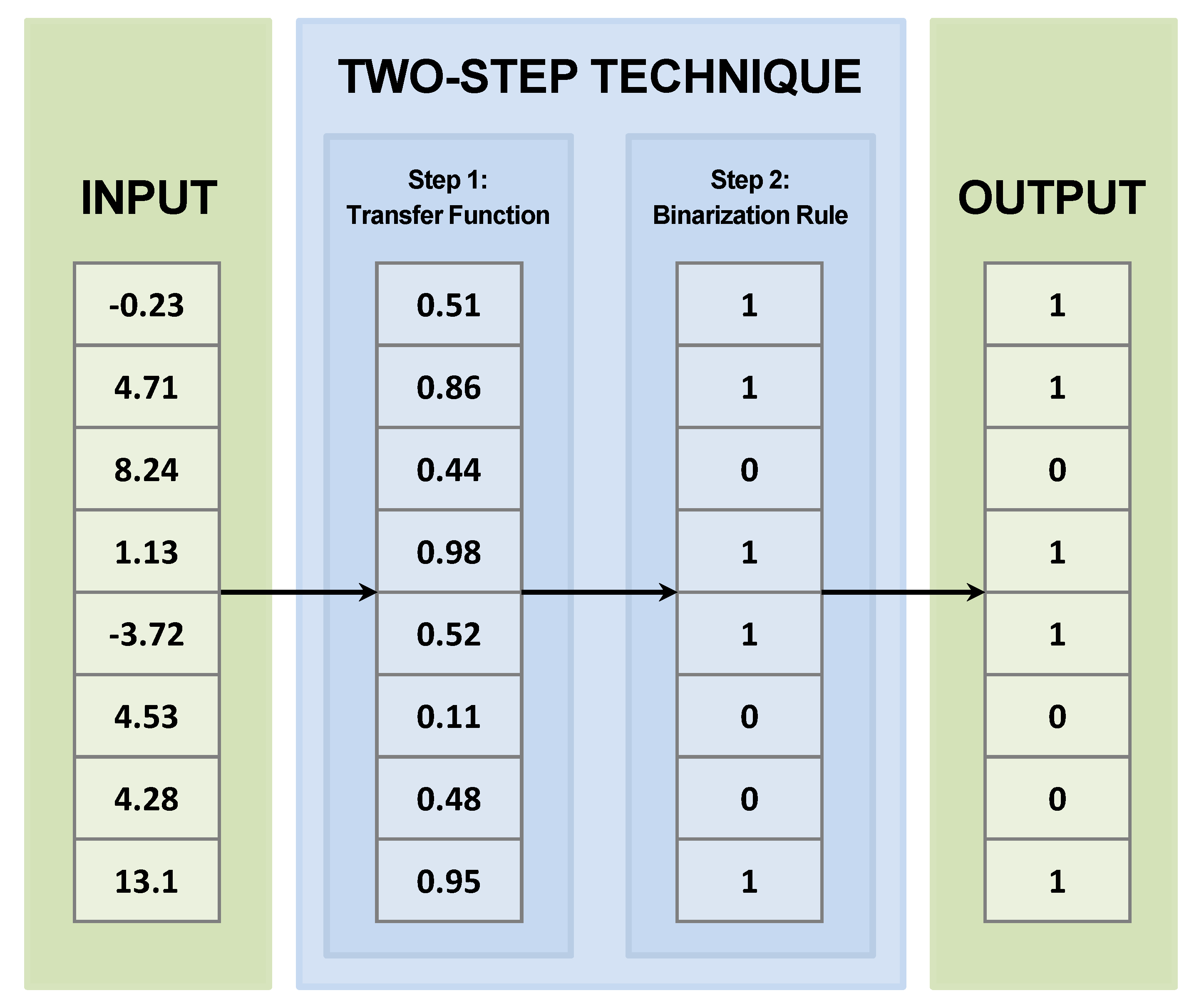
4.1. Two−Step Techniques
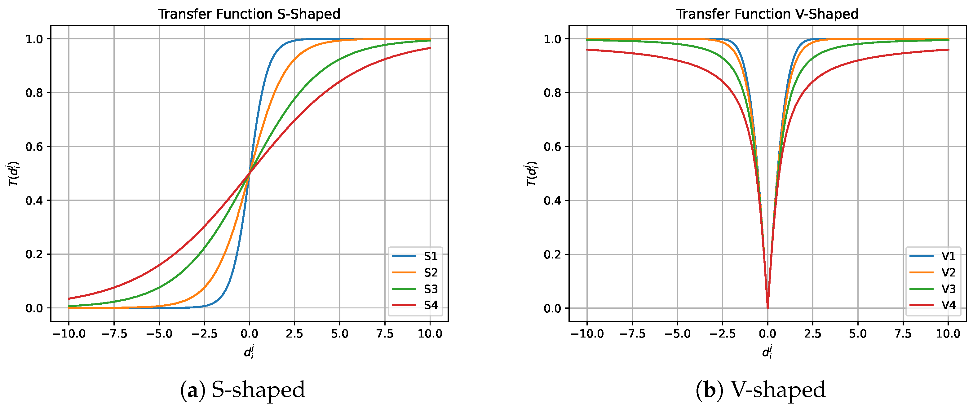
4.1.1. Transfer Function
4.1.2. Binarization Rule
| Algorithm 1 Two-step technique. |
Input: Continuous population Output: Binary population
|
4.2. Binary Particle Swarm Optimization
| Algorithm 2 Binary Particle Swarm Optimization. |
Input: The population Output: The updated population and
|
4.3. Binary Grey Wolf Optimizer
| Algorithm 3 Binary Grey Wolf Optimizer. |
Input: The population Output: The updated population and
|
4.4. Binary Pendulum Search Algorithm
| Algorithm 4 Binary Pendulum Search Algorithm. |
Input: The population Output: The updated population and
|
4.5. Binary Whale Optimization Algorithm
4.5.1. Searching for Prey
4.5.2. Encircling the Prey
4.5.3. Spiral Movement
| Algorithm 5 Binary Whale Optimization Algorithm. |
Input: The population Output: The updated population and
|
5. Enhanced Prediction of IDH Through ML and Biomarker Analysis
5.1. Addressing the Imbalance in the Dataset
5.2. Construction of Objective Function
| Algorithm 6 Objective function. |
Input: Selected features and dataset Output: Objective function and performance metrics
|
5.3. Selection of Classifiers
5.4. Metaheuristics for Feature Selection
6. Results
6.1. Experiment Configuration
6.1.1. Sampling Parameters
6.1.2. Classifiers Parameters
6.1.3. Metaheuristic Configuration
6.1.4. Objective Function
- is a weight parameter set to 0.99 in this experiment.
- represents the classification error metric.
- represents the proportion of selected features.
- Objective Function 1 (OF1)Recall macro is the simple recall average for both classes, representing the ratio of false negatives overall, NSF is the number of selected features, and TNF is the total number of features.
- Objective Function 2 (OF2)where recall minority represents the ratio of false negatives in the minority class, and as in Objective Function 1, NSF is the number of selected features, and TNF is the total number of features.
6.1.5. Experimentation Environment
6.2. Evaluation Criteria
6.2.1. Macro Metrics
- F-score (f1_m): The F-score is the harmonic mean of precision and recall, providing a single metric that balances both. It is calculated as
- Recall Macro (r_m): Recall macro is the average recall score over all classes, considering class imbalance by treating all classes equally. It is defined aswhere and represent the true positives and false negatives for each class i, and n is the number of classes.
- Precision Macro (p_m): Precision macro is the average precision score over all classes. It is defined aswhere and are the true positives and false positives for each class i, and n is the number of classes.
6.2.2. Class-Specific Metrics
Minority Class Metrics
- F-score minority (f_min): The F-score for the minority class, calculated similarly to the macro F-score, focuses specifically on the performance of the minority class:
- Recall minority (r_min): Recall for the minority class measures how well the minority class is identified:
- Precision Minority (p_min): Precision for the minority class measures the accuracy of positive predictions for the minority class:
Majority Class Metrics
- F-score majority (f1_may): The F-score for the majority class, calculated similarly to the macro F-score, focuses on the majority class:
- Recall majority (r_may): Recall for the majority class measures how well the majority class is identified:
- Precision majority (p_may): Precision for the majority class measures the accuracy of positive predictions for the majority class:
6.2.3. Total Features Selected (TFS)
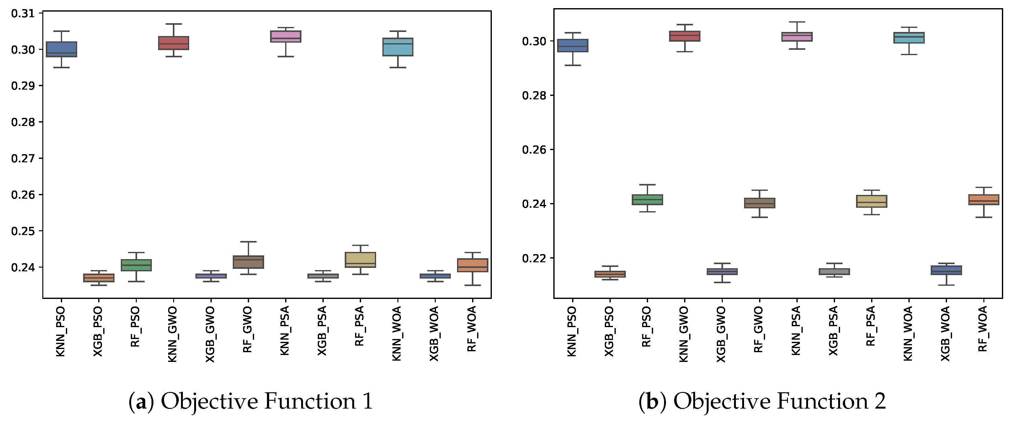
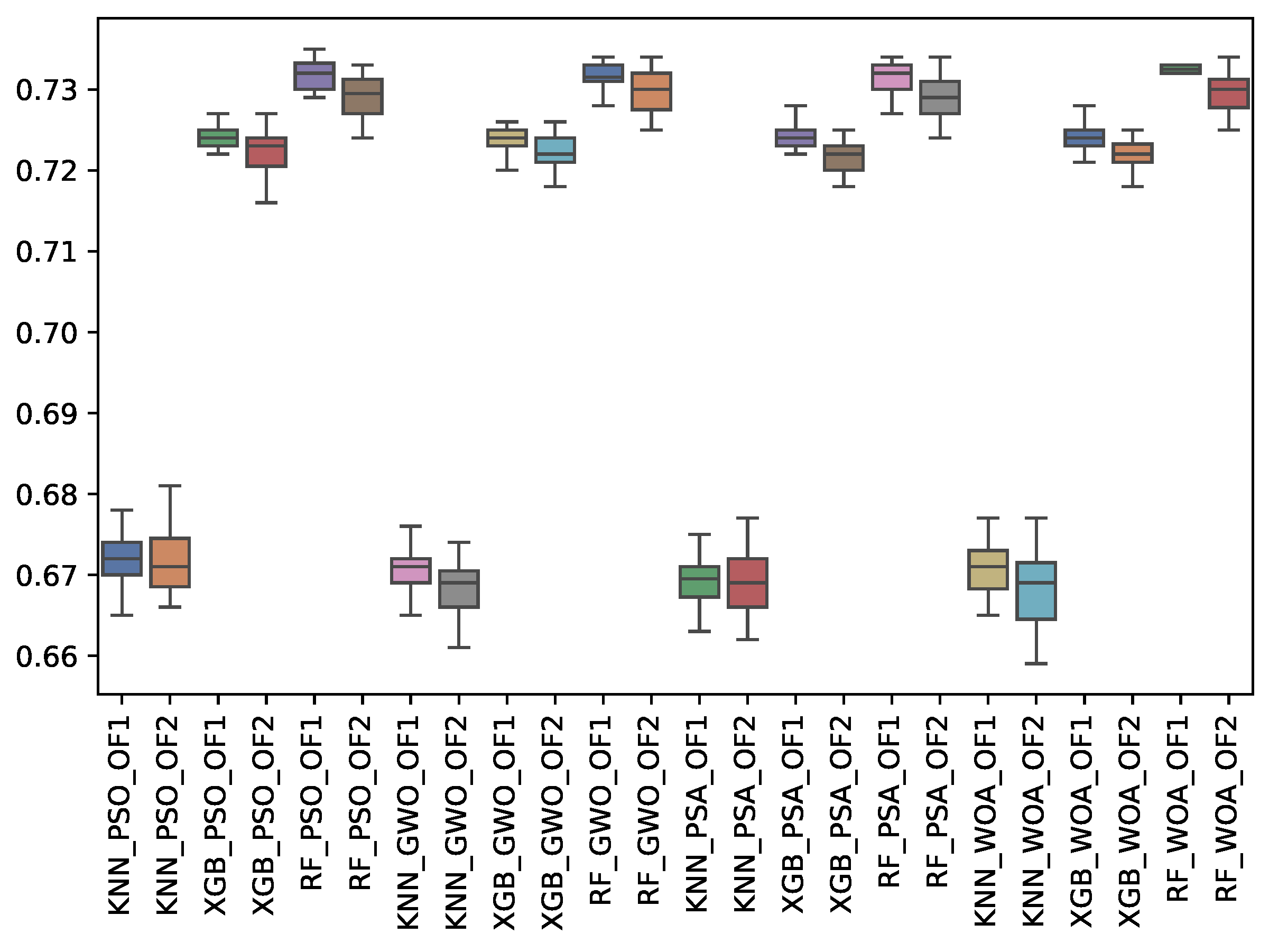
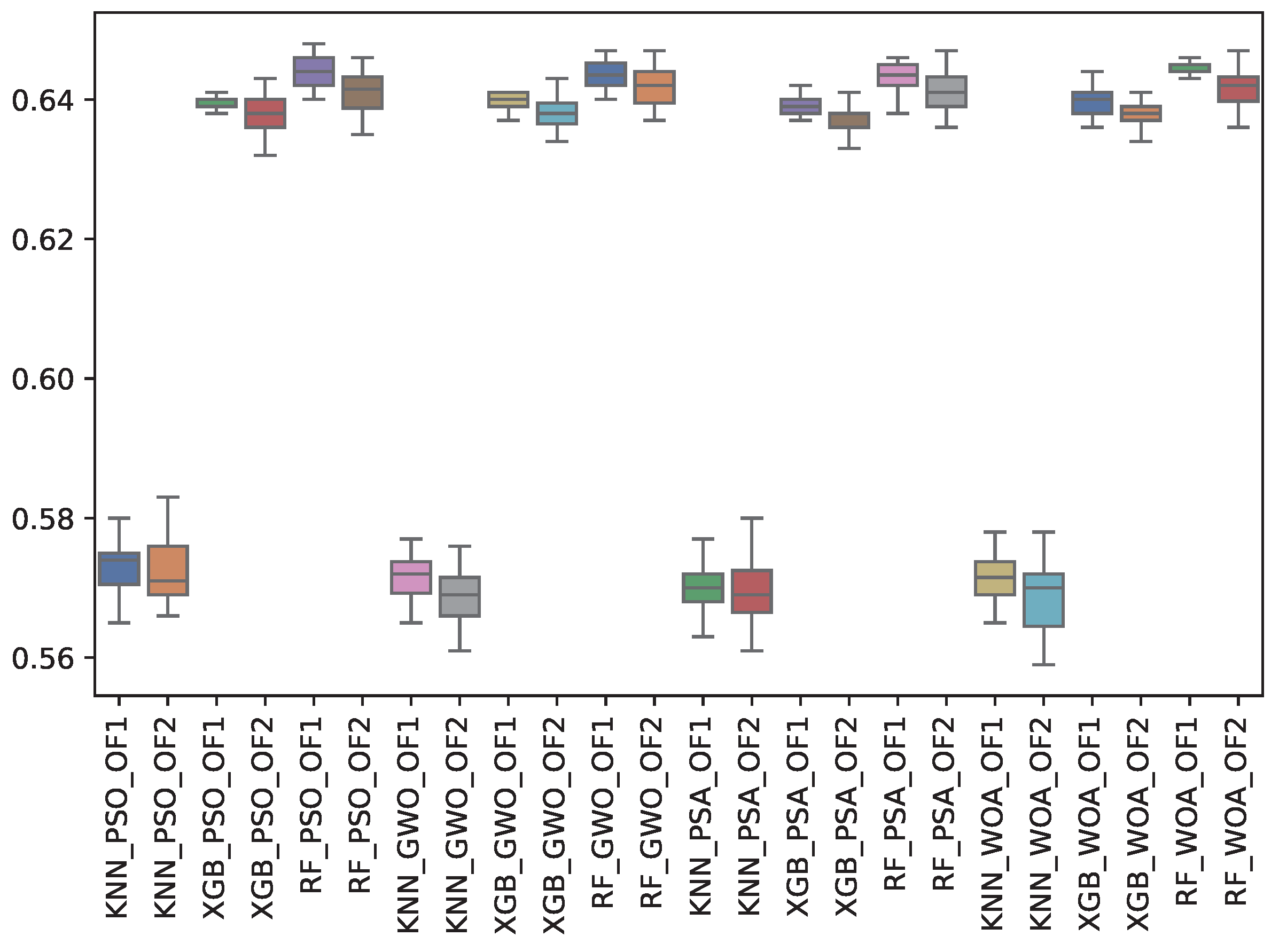
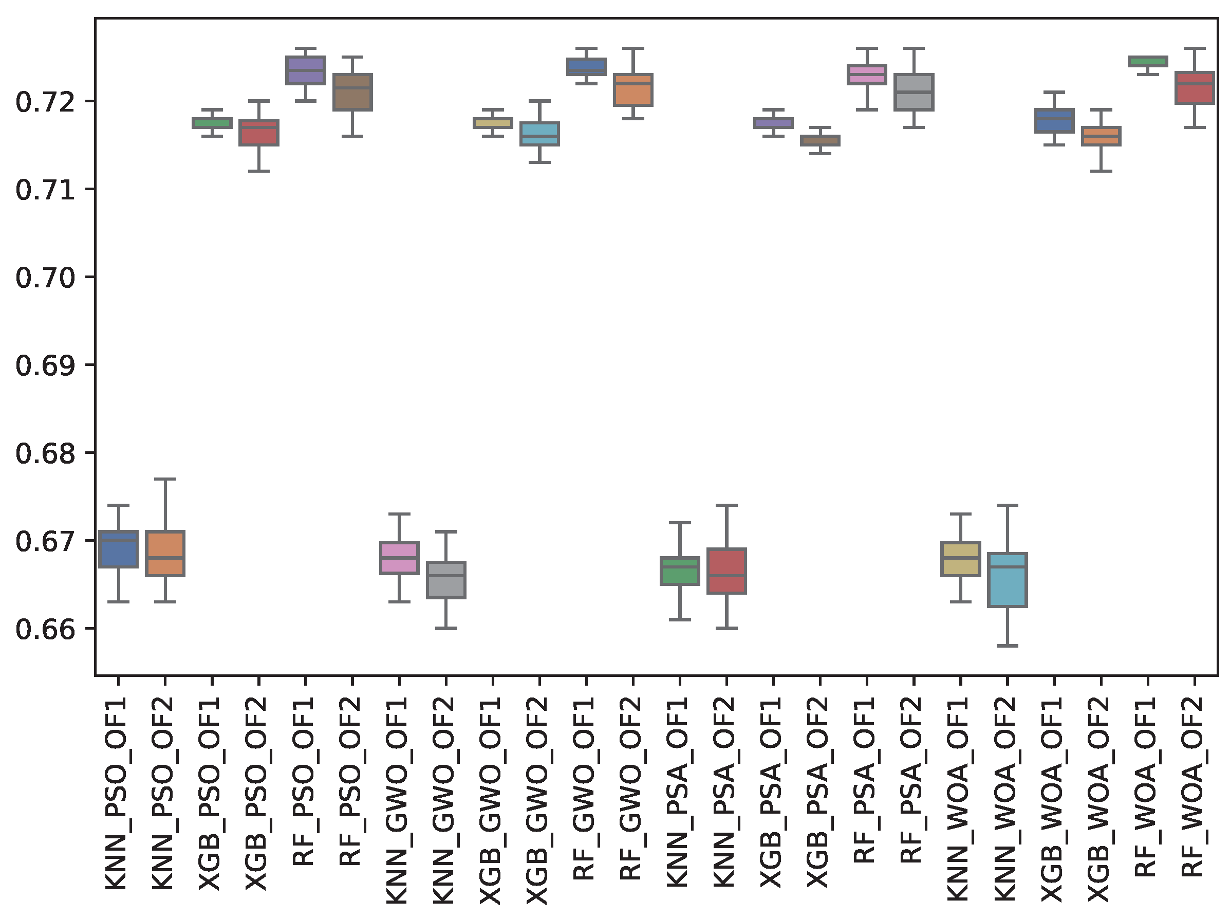
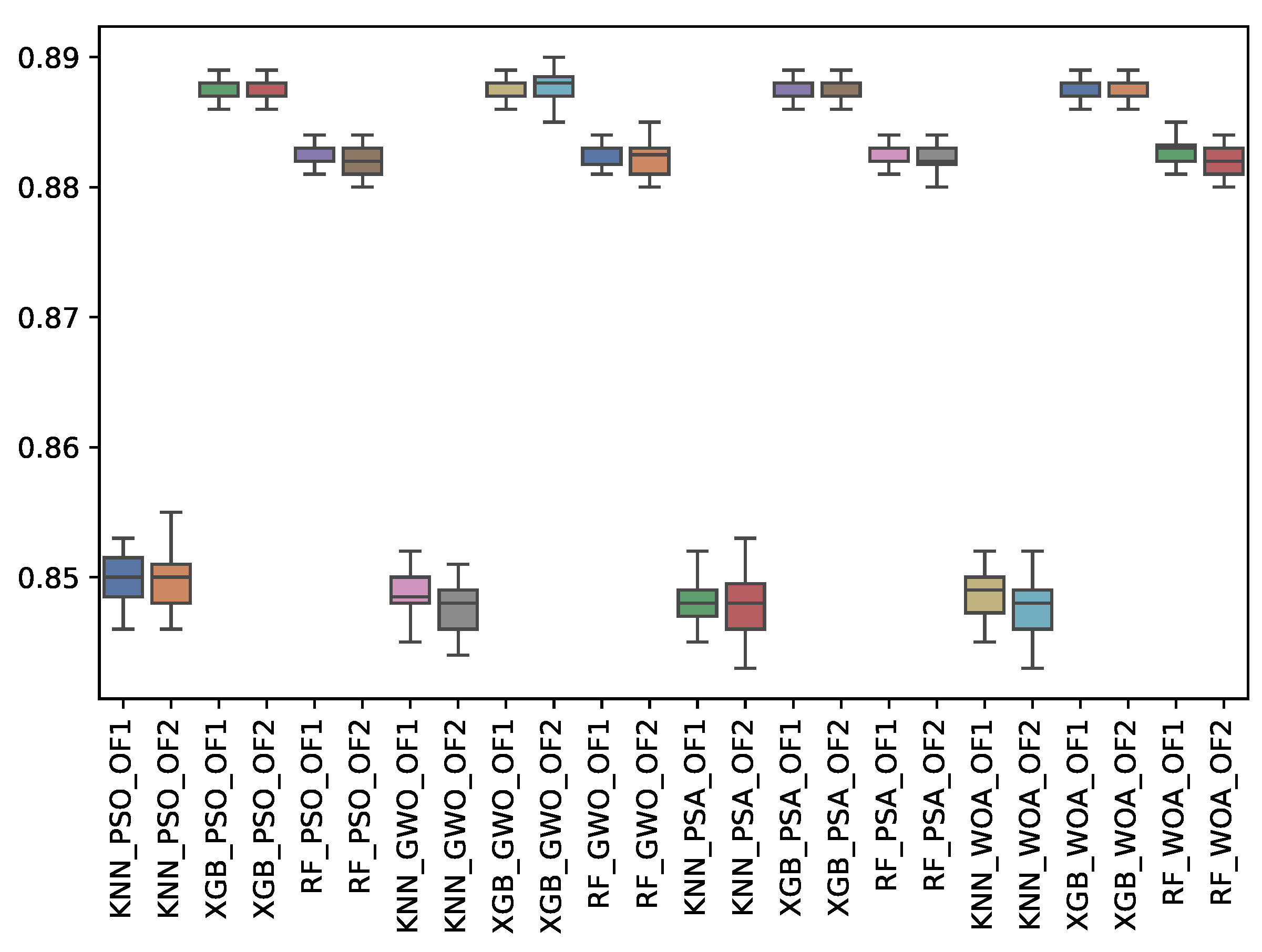
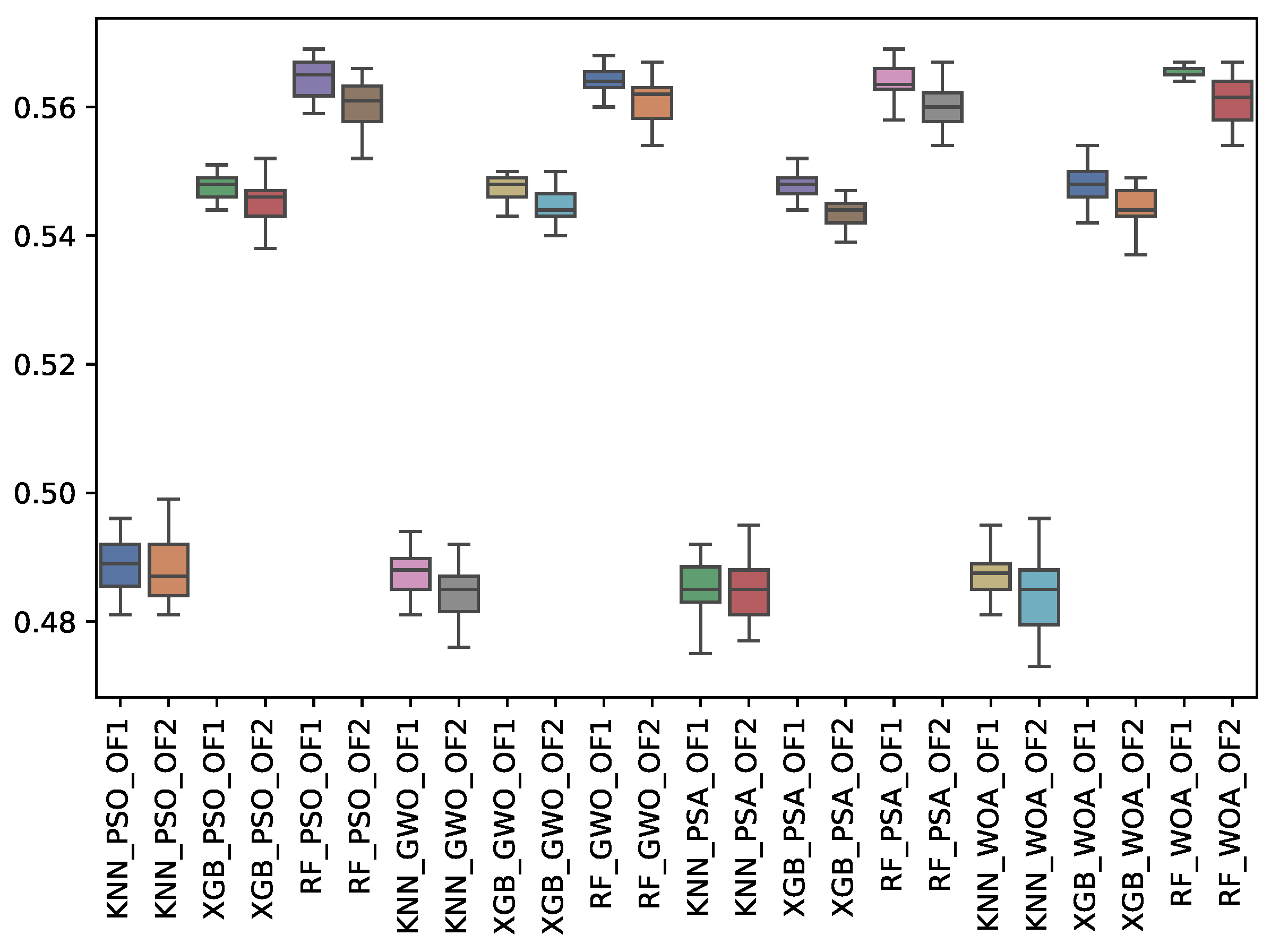
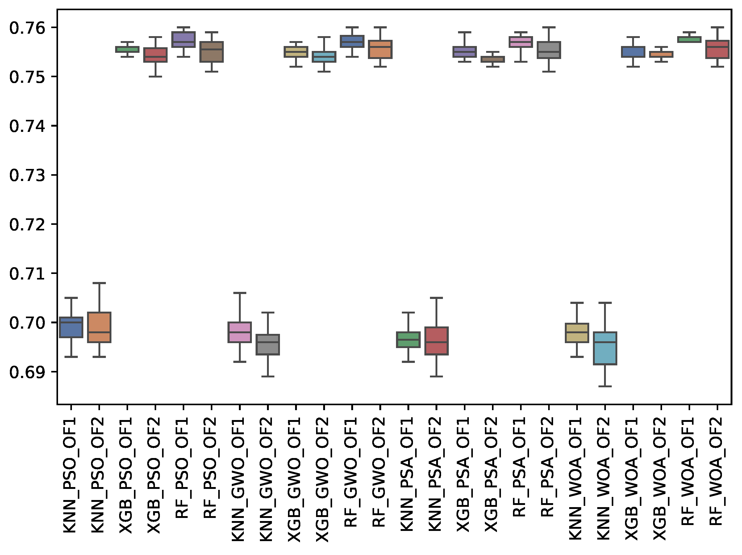
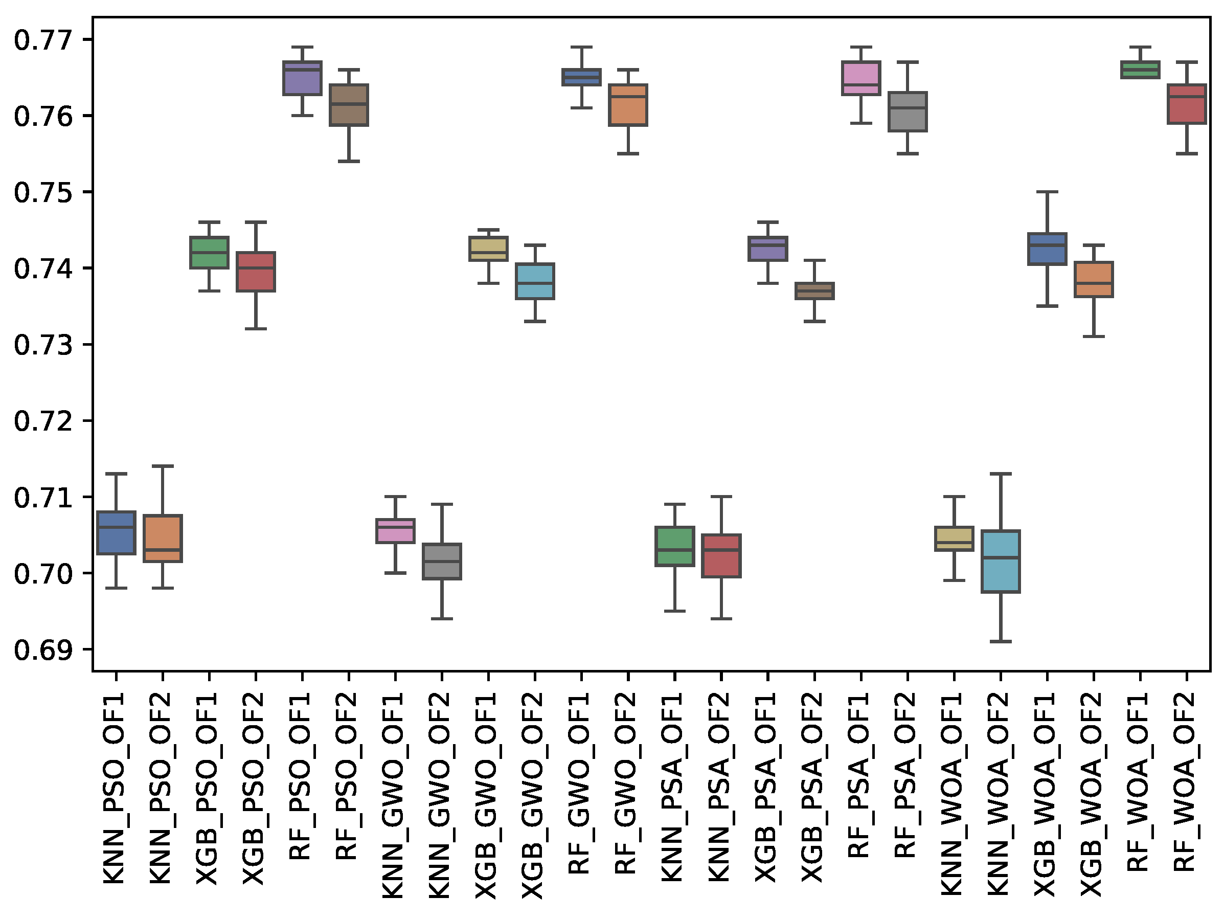
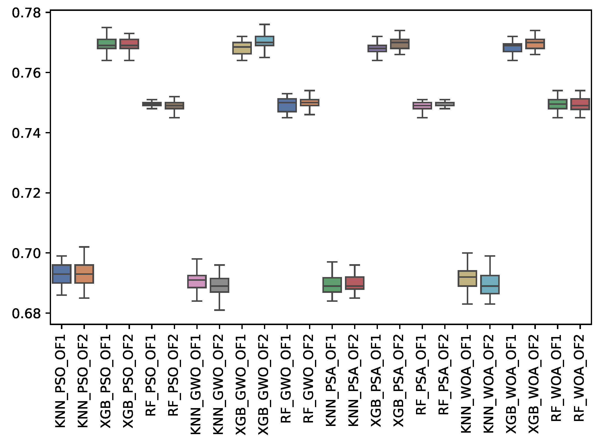
6.3. Experiment Results
6.4. Statistical Test
- Apply the Friedman test to determine if there is an overall statistical difference between all the algorithms.
- If the Friedman test is positive (p-value < 0.05), the Neminyi post hoc test is applied to identify the pairs of algorithms with statistical differences.
- Once the pairs have a statistical difference, the Wilcoxon signed-rank test will be applied to determine the directionality of the statistical difference, that is, to determine which algorithm is better than the other.
7. Conclusions
- Algorithm optimization beyond feature selection: In addition to feature selection, future studies could explore the optimization of hyperparameters of machine learning models.
- Application of deep learning models: Investigating the application of deep learning models, such as recurrent neural networks (RNNs) or long short-term memory networks (LSTMs), may provide further insight into complex relationships in the data and improve predictive accuracy.
- Personalized prediction models: Future research could focus on creating personalized prediction models based on individual patient profiles and climatic or geographic characteristics.
- Clinical validation and implementation: Validation through real-world clinical trials is necessary to bring the predictive model into clinical practice. This would involve integrating the model into dialysis machines or clinical decision support systems to assess its efficacy in a live healthcare setting. This gives rise to another future research oriented towards Explainable Artificial Intelligence. With this, models seek to be interpretable by professionals outside the field, such as medical professionals.
Author Contributions
Funding
Data Availability Statement
Acknowledgments
Conflicts of Interest
References
- Sociedad Española de Nefrología. La Enfermedad Renal Crónica en España 2023. 2023. Available online: https://www.xn--diamundialdelrion-txb.com/wp-content/uploads/2023/03/SEN_dossier_DMR2023.pdf (accessed on 12 July 2024).
- Arrieta, J.; Rodriguez-Carmona, A.; Remon, C.; Pérez-Fontán, M.; Ortega, F.; Sanchez-Tomero, J.A.; Selgas, R. Cost comparison between haemodialysis and peritoneal dialysis outsourcing agreements. Nefrol. Publ. Of. Soc. Esp. Nefrol. 2012, 32, 247–248. [Google Scholar]
- Kuipers, J.; Verboom, L.M.; Ipema, K.J.; Paans, W.; Krijnen, W.P.; Gaillard, C.A.; Westerhuis, R.; Franssen, C.F. The prevalence of intradialytic hypotension in patients on conventional hemodialysis: A systematic review with meta-analysis. Am. J. Nephrol. 2019, 49, 497–506. [Google Scholar] [CrossRef] [PubMed]
- Flythe, J.E.; Chang, T.I.; Gallagher, M.P.; Lindley, E.; Madero, M.; Sarafidis, P.A.; Unruh, M.L.; Wang, A.Y.M.; Weiner, D.E.; Cheung, M.; et al. Blood pressure and volume management in dialysis: Conclusions from a Kidney Disease: Improving Global Outcomes (KDIGO) Controversies Conference. Kidney Int. 2020, 97, 861–876. [Google Scholar] [CrossRef]
- Furaz Czerpak, K.R.; Puente García, A.; Corchete Prats, E.; Moreno de la Higuera, M.; Gruss Vergara, E.; Martín-Hernández, R. Estrategias para el control de la hipotensión en hemodiálisis. Nefrología 2014, 6, 1–14. [Google Scholar]
- Agarwal, R. How can we prevent intradialytic hypotension? Curr. Opin. Nephrol. Hypertens. 2012, 21, 593–599. [Google Scholar] [CrossRef]
- Aceto, G.; Persico, V.; Pescapé, A. Industry 4.0 and health: Internet of things, big data, and cloud computing for healthcare 4.0. J. Ind. Inf. Integr. 2020, 18, 100129. [Google Scholar] [CrossRef]
- Gambhir, S.; Malik, S.K.; Kumar, Y. Role of soft computing approaches in healthcare domain: A mini review. J. Med Syst. 2016, 40, 1–20. [Google Scholar] [CrossRef]
- Rayan, Z.; Alfonse, M.; Salem, A.B.M. Machine learning approaches in smart health. Procedia Comput. Sci. 2019, 154, 361–368. [Google Scholar] [CrossRef]
- Slon Roblero, M.F.; Bajo Rubio, M.A.; Gonzalez-Moya, M.; Calvino Varela, J.; Perez Alba, A.; Villaro Gumpert, J.; Cigarran, S.; Vidau, P.; Garcia Marcos, S.; Abaigar Luquin, P.; et al. Experience in Spain with the first patients in home hemodialysis treated with low-flow dialysate monitors. Nefrologia 2022, 42, 460–470. [Google Scholar] [CrossRef]
- Gilissen, J.; Pivodic, L.; Unroe, K.T.; Van den Block, L. International COVID-19 palliative care guidance for nursing homes leaves key themes unaddressed. J. Pain Symptom Manag. 2020, 60, e56–e69. [Google Scholar] [CrossRef]
- Lim, C.; Kim, K.J.; Maglio, P.P. Smart cities with big data: Reference models, challenges, and considerations. Cities 2018, 82, 86–99. [Google Scholar] [CrossRef]
- Zadeh, L.A. Soft computing and fuzzy logic. IEEE Softw. 1994, 11, 48–56. [Google Scholar] [CrossRef]
- Ibrahim, D. An overview of soft computing. Procedia Comput. Sci. 2016, 102, 34–38. [Google Scholar] [CrossRef]
- Tamboli, S.; Bewoor, L. A review of soft computing technique for real-time data forecasting. In Proceedings of the International Conference on Communication and Information Processing (ICCIP), Chongqing, China, 15–17 November 2019. [Google Scholar]
- Binitha, S.; Sathya, S.S. A survey of bio inspired optimization algorithms. Int. J. Soft Comput. Eng. 2012, 2, 137–151. [Google Scholar]
- Sharma, D.; Chandra, P. A comparative analysis of soft computing techniques in software fault prediction model development. Int. J. Inf. Technol. 2019, 11, 37–46. [Google Scholar] [CrossRef]
- Santos, F.A.O.; de Jesus, G.S.; Botelho, G.A.; Macedo, H.T. Smart health: Using fuzzy logic in the monitoring of health-related indicators. In Proceedings of the 2016 8th Euro American Conference on Telematics and Information Systems (EATIS), Cartagena, Colombia, 28–29 April 2016; IEEE: Piscataway, NJ, USA, 2016; pp. 1–4. [Google Scholar]
- Mehta, R. Multivariate Fuzzy Logic Based Smart Healthcare Monitoring for Risk Evaluation of Cardiac Patients. In Medical Informatics and Bioimaging Using Artificial Intelligence: Challenges, Issues, Innovations and Recent Developments; Springer: Cham, Switzerland, 2022; pp. 219–243. [Google Scholar]
- Alkeshuosh, A.H.; Moghadam, M.Z.; Al Mansoori, I.; Abdar, M. Using PSO algorithm for producing best rules in diagnosis of heart disease. In Proceedings of the 2017 International Conference on Computer and Applications (ICCA), Doha, Qatar, 6–7 September 2017; IEEE: Piscataway, NJ, USA, 2017; pp. 306–311. [Google Scholar]
- Mansour, R.F. Evolutionary computing enriched computer-aided diagnosis system for diabetic retinopathy: A survey. IEEE Rev. Biomed. Eng. 2017, 10, 334–349. [Google Scholar] [CrossRef]
- Kumar, S.; Nayyar, A.; Paul, A. Swarm Intelligence and Evolutionary Algorithms in Healthcare and Drug Development; CRC Press: Boca Raton, FL, USA, 2019. [Google Scholar]
- Jasmine Gabriel, J.; Jani Anbarasi, L. Evolutionary computing-based feature selection for cardiovascular disease: A review. In International Virtual Conference on Industry 4.0: Select Proceedings of IVCI4.0 2020; Springer: Singapore, 2021; pp. 47–56. [Google Scholar]
- Kumar, T.A.; Rajmohan, R.; Pavithra, M.; Balamurugan, S. Evolutionary Intelligence for Healthcare Applications; CRC Press: Boca Raton, FL, USA, 2022. [Google Scholar]
- Di Biasi, L.; De Marco, F.; Auriemma Citarella, A.; Barra, P.; Piotto Piotto, S.; Tortora, G. Hybrid Approach for the Design of CNNs Using Genetic Algorithms for Melanoma Classification. In Proceedings of the Pattern Recognition, Computer Vision, and Image Processing. ICPR 2022 International Workshops and Challenges, Montreal, QC, Canada, 21–25 August 2022; Proceedings, Part I. Springer: Berlin/Heidelberg, Germany, 2022; pp. 514–528. [Google Scholar] [CrossRef]
- Gupta, S.; Sedamkar, R. Machine learning for healthcare: Introduction. In Machine Learning with Health Care Perspective: Machine Learning and Healthcare; Springer: Cham, Switzerland, 2020; pp. 1–25. [Google Scholar]
- Nayyar, A.; Gadhavi, L.; Zaman, N. Machine learning in healthcare: Review, opportunities and challenges. In Machine Learning and the Internet of Medical Things in Healthcare; Springer: Cham, Switzerland, 2021; pp. 23–45. [Google Scholar]
- Usmani, U.A.; Jaafar, J. Machine learning in healthcare: Current trends and the future. In Proceedings of the International Conference on Artificial Intelligence for Smart Community: AISC 2020, Universiti Teknologi Petronas, Seri Iskandar, Malaysia, 17–18 December 2020; Springer: Cham, Switzerland, 2022; pp. 659–675. [Google Scholar]
- Kaur, P.; Kumar, R.; Kumar, M. A healthcare monitoring system using random forest and internet of things (IoT). Multimed. Tools Appl. 2019, 78, 19905–19916. [Google Scholar] [CrossRef]
- Haglin, J.M.; Jimenez, G.; Eltorai, A.E. Artificial neural networks in medicine. Health Technol. 2019, 9, 1–6. [Google Scholar] [CrossRef]
- Lisboa, P.J.; Ifeachor, E.C.; Szczepaniak, P.S. Artificial Neural Networks in Biomedicine; Springer Science & Business Media: Berlin, Germany, 2000. [Google Scholar]
- Filist, S.; Al-Kasasbeh, R.T.; Shatalova, O.; Aikeyeva, A.; Korenevskiy, N.; Shaqadan, A.; Trifonov, A.; Ilyash, M. Developing neural network model for predicting cardiac and cardiovascular health using bioelectrical signal processing. Comput. Methods Biomech. Biomed. Eng. 2022, 25, 908–921. [Google Scholar] [CrossRef]
- LeCun, Y.; Bengio, Y.; Hinton, G. Deep learning. Nature 2015, 521, 436–444. [Google Scholar] [CrossRef]
- Sujith, A.; Sajja, G.S.; Mahalakshmi, V.; Nuhmani, S.; Prasanalakshmi, B. Systematic review of smart health monitoring using deep learning and Artificial intelligence. Neurosci. Inform. 2022, 2, 100028. [Google Scholar] [CrossRef]
- Yang, S.; Zhu, F.; Ling, X.; Liu, Q.; Zhao, P. Intelligent health care: Applications of deep learning in computational medicine. Front. Genet. 2021, 12, 607471. [Google Scholar] [CrossRef] [PubMed]
- Iyortsuun, N.K.; Kim, S.H.; Jhon, M.; Yang, H.J.; Pant, S. A review of machine learning and deep learning approaches on mental health diagnosis. Healthcare 2023, 11, 285. [Google Scholar] [CrossRef] [PubMed]
- Singh, K.; Malhotra, J. Deep learning based smart health monitoring for automated prediction of epileptic seizures using spectral analysis of scalp EEG. Phys. Eng. Sci. Med. 2021, 44, 1161–1173. [Google Scholar] [CrossRef]
- Shafi, J.; Obaidat, M.S.; Krishna, P.V.; Sadoun, B.; Pounambal, M.; Gitanjali, J. Prediction of heart abnormalities using deep learning model and wearabledevices in smart health homes. Multimed. Tools Appl. 2022, 81, 543–557. [Google Scholar] [CrossRef]
- Zitzler, E.; Deb, K.; Thiele, L. Comparison of Multiobjective Evolutionary Algorithms: Empirical Results. Evol. Comput. 2000, 8, 173–195. [Google Scholar] [CrossRef]
- Haupt, R.L.; Haupt, S.E. Practical Genetic Algorithms; John Wiley & Sons: Hoboken, NJ, USA, 2004. [Google Scholar]
- Houssein, E.H.; Saber, E.; Ali, A.A.; Wazery, Y.M. Integrating metaheuristics and artificial intelligence for healthcare: Basics, challenging and future directions. Artif. Intell. Rev. 2024, 57, 205. [Google Scholar] [CrossRef]
- Kaur, S.; Kumar, Y.; Koul, A.; Kumar Kamboj, S. A systematic review on metaheuristic optimization techniques for feature selections in disease diagnosis: Open issues and challenges. Arch. Comput. Methods Eng. 2023, 30, 1863–1895. [Google Scholar] [CrossRef]
- Hong, D.; Chang, H.; He, X.; Zhan, Y.; Tong, R.; Wu, X.; Li, G. Construction of an Early Alert System for Intradialytic Hypotension before Initiating Hemodialysis Based on Machine Learning. Kidney Dis. 2023, 9, 433–442. [Google Scholar] [CrossRef]
- Gervasoni, F.; Bellocchio, F.; Rosenberger, J.; Arkossy, O.; Ion Titapiccolo, J.; Kovarova, V.; Larkin, J.; Nikam, M.; Stuard, S.; Tripepi, G.L.; et al. Development and validation of AI-based triage support algorithms for prevention of intradialytic hypotension. J. Nephrol. 2023, 36, 2001–2011. [Google Scholar] [CrossRef]
- Moeinzadeh, F.; Sattari, M. Proposed Method for Predicting COVID-19 Severity in Chronic Kidney Disease Patients Based on Ant Colony Algorithm and CHAID. J. Adv. Med Biomed. Res. 2022, 30, 507–512. [Google Scholar] [CrossRef]
- Yang, X.; Zhao, D.; Yu, F.; Heidari, A.A.; Bano, Y.; Ibrohimov, A.; Liu, Y.; Cai, Z.; Chen, H.; Chen, X. An optimized machine learning framework for predicting intradialytic hypotension using indexes of chronic kidney disease-mineral and bone disorders. Comput. Biol. Med. 2022, 145, 105510. [Google Scholar] [CrossRef] [PubMed]
- Othman, M.; Elbasha, A.M.; Naga, Y.S.; Moussa, N.D. Early prediction of hemodialysis complications employing ensemble techniques. BioMedical Eng. Online 2022, 21, 74. [Google Scholar] [CrossRef] [PubMed]
- Nafisi, V.R.; Shahabi, M. Intradialytic hypotension related episodes identification based on the most effective features of photoplethysmography signal. Comput. Methods Programs Biomed. 2018, 157, 1–9. [Google Scholar] [CrossRef] [PubMed]
- Arienzo, G.; Citarella, A.A.; De Marco, F.; De Roberto, A.M.; Di Biasi, L.; Francese, R.; Tortora, G. Cardioview: A framework for detection premature ventricular contractions with explainable artificial intelligence. In Proceedings of the INI-DH 2024: Workshop on Innovative Interfaces in Digital Healthcare, in Conjunction with International Conference on Advanced Visual Interfaces, Genoa, Italy, 3–7 June 2024; pp. 3–7. [Google Scholar]
- De Marco, F.; Di Biasi, L.; Auriemma Citarella, A.; Tortora, G. Improving pvc detection in ecg signals: A recurrent neural network approach. In Proceedings of the Italian Workshop on Artificial Life and Evolutionary Computation, Venice, Italy, 6–8 September 2023; Springer: Berlin/Heidelberg, Germany, 2023; pp. 256–267. [Google Scholar]
- Mendoza-Pittí, L.; Gómez-Pulido, J.M.; Vargas-Lombardo, M.; Gómez-Pulido, J.A.; Polo-Luque, M.L.; Rodréguez-Puyol, D. Machine-learning model to predict the intradialytic hypotension based on clinical-analytical data. IEEE Access 2022, 10, 72065–72079. [Google Scholar] [CrossRef]
- Cheripurathu, K.G.; Kulkarni, S. Integrating Microservices and Microfrontends: A Comprehensive Literature Review on Architecture, Design Patterns, and Implementation Challenges. J. Sci. Res. Technol. 2024, 2, 1–12. [Google Scholar]
- Chowdhury, M.Z.I.; Turin, T.C. Variable selection strategies and its importance in clinical prediction modelling. Fam. Med. Community Health 2020, 8, e000262. [Google Scholar] [CrossRef]
- Steyerberg, E.W.; Vergouwe, Y. Towards better clinical prediction models: Seven steps for development and an ABCD for validation. Eur. Heart J. 2014, 35, 1925–1931. [Google Scholar] [CrossRef]
- Mehrpoor, G.; Azimzadeh, M.M.; Monfared, A. Data mining: A novel outlook to explore knowledge in health and medical sciences. Int. J. Travel Med. Glob. Health 2014, 2, 87–90. [Google Scholar]
- Barrera-García, J.; Cisternas-Caneo, F.; Crawford, B.; Gómez Sánchez, M.; Soto, R. Feature selection problem and metaheuristics: A systematic literature review about its formulation, evaluation and applications. Biomimetics 2023, 9, 9. [Google Scholar] [CrossRef]
- Rajwar, K.; Deep, K.; Das, S. An exhaustive review of the metaheuristic algorithms for search and optimization: Taxonomy, applications, and open challenges. Artif. Intell. Rev. 2023, 56, 13187–13257. [Google Scholar] [CrossRef]
- Becerra-Rozas, M.; Lemus-Romani, J.; Cisternas-Caneo, F.; Crawford, B.; Soto, R.; Astorga, G.; Castro, C.; García, J. Continuous metaheuristics for binary optimization problems: An updated systematic literature review. Mathematics 2022, 11, 129. [Google Scholar] [CrossRef]
- Kennedy, J.; Eberhart, R.C. A discrete binary version of the particle swarm algorithm. In Proceedings of the 1997 IEEE International Conference on Systems, Man, and Cybernetics. Computational Cybernetics and Simulation, Orlando, FL, USA, 12–15 October 1997; IEEE: Piscataway, NJ, USA, 1997; Volume 5, pp. 4104–4108. [Google Scholar] [CrossRef]
- Mirjalili, S.; Lewis, A. S-shaped versus V-shaped transfer functions for binary particle swarm optimization. Swarm Evol. Comput. 2013, 9, 1–14. [Google Scholar] [CrossRef]
- Crawford, B.; Soto, R.; Astorga, G.; García, J.; Castro, C.; Paredes, F. Putting continuous metaheuristics to work in binary search spaces. Complexity 2017, 2017, 8404231. [Google Scholar] [CrossRef]
- Lanza-Gutierrez, J.M.; Crawford, B.; Soto, R.; Berrios, N.; Gomez-Pulido, J.A.; Paredes, F. Analyzing the effects of binarization techniques when solving the set covering problem through swarm optimization. Expert Syst. Appl. 2017, 70, 67–82. [Google Scholar] [CrossRef]
- Kennedy, J.; Eberhart, R. Particle swarm optimization. In Proceedings of the ICNN’95-International Conference on Neural Networks, Perth, WA, Australia, 27 November–1 December 1995; IEEE: Piscataway, NJ, USA, 1995; Volume 4, pp. 1942–1948. [Google Scholar]
- Mirjalili, S.; Mirjalili, S.M.; Lewis, A. Grey wolf optimizer. Adv. Eng. Softw. 2014, 69, 46–61. [Google Scholar] [CrossRef]
- Lemus-Romani, J.; Becerra-Rozas, M.; Crawford, B.; Soto, R.; Cisternas-Caneo, F.; Vega, E.; Castillo, M.; Tapia, D.; Astorga, G.; Palma, W.; et al. A novel learning-based binarization scheme selector for swarm algorithms solving combinatorial problems. Mathematics 2021, 9, 2887. [Google Scholar] [CrossRef]
- Ab. Aziz, N.A.; Ab. Aziz, K. Pendulum Search Algorithm: An Optimization Algorithm Based on Simple Harmonic Motion and Its Application for a Vaccine Distribution Problem. Algorithms 2022, 15, 214. [Google Scholar] [CrossRef]
- Crawford, B.; Cisternas-Caneo, F.; Sepúlveda, K.; Soto, R.; Paz, Á.; Peña, A.; León de la Barra, C.; Rodriguez-Tello, E.; Astorga, G.; Castro, C.; et al. B-PSA: A Binary Pendulum Search Algorithm for the Feature Selection Problem. Computers 2023, 12, 249. [Google Scholar] [CrossRef]
- Mirjalili, S.; Lewis, A. The whale optimization algorithm. Adv. Eng. Softw. 2016, 95, 51–67. [Google Scholar] [CrossRef]
- Lemaître, G.; Nogueira, F.; Aridas, C.K. Imbalanced-learn: A Python Toolbox to Tackle the Curse of Imbalanced Datasets in Machine Learning. J. Mach. Learn. Res. 2017, 18, 1–5. [Google Scholar]
- Agrawal, P.; Abutarboush, H.F.; Ganesh, T.; Mohamed, A.W. Metaheuristic Algorithms on Feature Selection: A Survey of One Decade of Research (2009–2019). IEEE Access 2021, 9, 26766–26791. [Google Scholar] [CrossRef]
- Igel, C. No Free Lunch Theorems: Limitations and Perspectives of Metaheuristics. In Theory and Principled Methods for the Design of Metaheuristics; Borenstein, Y., Moraglio, A., Eds.; Springer: Berlin/Heidelberg, Germany, 2014; pp. 1–23. [Google Scholar] [CrossRef]
- Ho, Y.C.; Pepyne, D.L. Simple explanation of the no-free-lunch theorem and its implications. J. Optim. Theory Appl. 2002, 115, 549–570. [Google Scholar] [CrossRef]
- Wolpert, D.; Macready, W. No free lunch theorems for optimization. IEEE Trans. Evol. Comput. 1997, 1, 67–82. [Google Scholar] [CrossRef]
- Pedregosa, F.; Varoquaux, G.; Gramfort, A.; Michel, V.; Thirion, B.; Grisel, O.; Blondel, M.; Prettenhofer, P.; Weiss, R.; Dubourg, V.; et al. Scikit-learn: Machine Learning in Python. J. Mach. Learn. Res. 2011, 12, 2825–2830. [Google Scholar]
- Chen, T.; Guestrin, C. XGBoost: A Scalable Tree Boosting System. In Proceedings of the 22nd ACM SIGKDD International Conference on Knowledge Discovery and Data Mining, New York, NY, USA, 13–17 August 2016; KDD ’16. pp. 785–794. [Google Scholar] [CrossRef]
- Hays, W.L.; Winkler, R.L. Statistics: Probability, Inference, and Decision; Holt, Rinehart and Winston: Austin, TX, USA, 1970. [Google Scholar]


| Labels | Features | ||||
|---|---|---|---|---|---|
| Instances | Non Hypotensive | Hypotensive | Pre. | Post. | |
| IDH dataset | 68,574 | 48,764 (71.11%) | 19,810 (28.89%) | 71 | 87 |
| Classifier | f1_m | r_m | p_m | fs_min | r_min | p_min | fs_may | r_may | p_may |
|---|---|---|---|---|---|---|---|---|---|
| XGBoost | 0.737 | 0.721 | 0.769 | 0.607 | 0.529 | 0.711 | 0.867 | 0.913 | 0.827 |
| RF | 0.717 | 0.698 | 0.763 | 0.570 | 0.474 | 0.715 | 0.864 | 0.923 | 0.812 |
| KNN | 0.651 | 0.641 | 0.677 | 0.474 | 0.405 | 0.571 | 0.828 | 0.876 | 0.784 |
| S-Shaped | V-Shaped | ||
|---|---|---|---|
| Name | Equation | Name | Equation |
| S1 | V1 | ||
| S2 | V2 | ||
| S3 | V3 | ||
| S4 | V4 | ||
| Type | Binarization Rules |
|---|---|
| Standard | |
| Complement | |
| Static Probability | |
| Elitist | |
| Roulette Elitist |
| Classifier | Parameter | f1_m | r_m | p_m | f1_min | r_min | p_min | f1_may | r_may | p_may |
|---|---|---|---|---|---|---|---|---|---|---|
| KNN | 1.0 | 0.632 | 0.659 | 0.634 | 0.527 | 0.652 | 0.443 | 0.737 | 0.666 | 0.825 |
| Random Forest | 1.0 | 0.72 | 0.746 | 0.712 | 0.629 | 0.738 | 0.549 | 0.81 | 0.753 | 0.876 |
| XGBoost | 1.0 | 0.725 | 0.756 | 0.718 | 0.64 | 0.766 | 0.549 | 0.81 | 0.745 | 0.887 |
| KNN | 0.9 | 0.64 | 0.66 | 0.638 | 0.526 | 0.622 | 0.455 | 0.754 | 0.698 | 0.82 |
| Random Forest | 0.9 | 0.727 | 0.745 | 0.718 | 0.631 | 0.709 | 0.568 | 0.822 | 0.781 | 0.869 |
| XGBoost | 0.9 | 0.734 | 0.758 | 0.725 | 0.645 | 0.745 | 0.569 | 0.823 | 0.771 | 0.881 |
| KNN | 0.8 | 0.646 | 0.66 | 0.642 | 0.523 | 0.59 | 0.47 | 0.769 | 0.729 | 0.814 |
| Random Forest | 0.8 | 0.732 | 0.743 | 0.725 | 0.63 | 0.677 | 0.59 | 0.834 | 0.809 | 0.86 |
| XGBoost | 0.8 | 0.739 | 0.756 | 0.731 | 0.646 | 0.718 | 0.587 | 0.833 | 0.795 | 0.874 |
| KNN | 0.7 | 0.652 | 0.659 | 0.648 | 0.519 | 0.553 | 0.488 | 0.786 | 0.765 | 0.808 |
| Random Forest | 0.7 | 0.734 | 0.737 | 0.732 | 0.625 | 0.636 | 0.613 | 0.843 | 0.837 | 0.85 |
| XGBoost | 0.7 | 0.744 | 0.753 | 0.737 | 0.645 | 0.686 | 0.609 | 0.843 | 0.821 | 0.866 |
| KNN | 0.6 | 0.655 | 0.655 | 0.655 | 0.509 | 0.508 | 0.509 | 0.8 | 0.801 | 0.8 |
| Random Forest | 0.6 | 0.736 | 0.73 | 0.743 | 0.618 | 0.593 | 0.646 | 0.854 | 0.868 | 0.84 |
| XGBoost | 0.6 | 0.745 | 0.745 | 0.745 | 0.638 | 0.64 | 0.636 | 0.852 | 0.851 | 0.853 |
| MH | Parameter | Value |
|---|---|---|
| PSO | 5000 | |
| 2 | ||
| 2 | ||
| 0.9 | ||
| 0.2 | ||
| GWO | a | decreases linearly from 2 to 0 |
| WOA | a | decreases linearly from 2 to 0 |
| b | 1 | |
| PSA | free parameters | |
| OF 1 | OF 2 | |||||||||||||||||
|---|---|---|---|---|---|---|---|---|---|---|---|---|---|---|---|---|---|---|
| KNN | RF | XGB | KNN | RF | XGB | |||||||||||||
| Fitness | Best | Avg. | Std. | Best | Avg. | Std. | Best | Avg. | Std. | Best | Avg. | Std. | Best | Avg. | Std. | Best | Avg. | Std. |
| GWO | 0.298 | 0.302 | 0.003 | 0.238 | 0.242 | 0.002 | 0.236 | 0.238 | 0.001 | 0.296 | 0.302 | 0.003 | 0.235 | 0.240 | 0.003 | 0.211 | 0.215 | 0.002 |
| PSA | 0.298 | 0.303 | 0.002 | 0.238 | 0.242 | 0.002 | 0.236 | 0.238 | 0.001 | 0.297 | 0.302 | 0.003 | 0.236 | 0.241 | 0.003 | 0.213 | 0.215 | 0.001 |
| PSO | 0.295 | 0.299 | 0.003 | 0.236 | 0.240 | 0.002 | 0.235 | 0.237 | 0.001 | 0.291 | 0.298 | 0.003 | 0.237 | 0.242 | 0.002 | 0.212 | 0.214 | 0.001 |
| WOA | 0.295 | 0.301 | 0.003 | 0.235 | 0.240 | 0.002 | 0.236 | 0.238 | 0.001 | 0.295 | 0.301 | 0.003 | 0.235 | 0.241 | 0.003 | 0.210 | 0.215 | 0.002 |
| OF 1 | OF 2 | |||||||||||
|---|---|---|---|---|---|---|---|---|---|---|---|---|
| KNN | RF | XGB | KNN | RF | XGB | |||||||
| f1_m | Avg. | Std. | Avg. | Std. | Avg. | Std. | Avg. | Std. | Avg. | Std. | Avg. | Std. |
| GWO | 0.671 | 0.002 | 0.732 | 0.002 | 0.724 | 0.001 | 0.668 | 0.004 | 0.730 | 0.003 | 0.722 | 0.002 |
| PSA | 0.669 | 0.003 | 0.731 | 0.002 | 0.724 | 0.001 | 0.669 | 0.004 | 0.729 | 0.002 | 0.721 | 0.002 |
| PSO | 0.672 | 0.003 | 0.732 | 0.002 | 0.724 | 0.001 | 0.671 | 0.004 | 0.729 | 0.003 | 0.722 | 0.003 |
| WOA | 0.671 | 0.003 | 0.732 | 0.001 | 0.724 | 0.002 | 0.668 | 0.004 | 0.729 | 0.003 | 0.722 | 0.002 |
| OF 1 | OF 2 | |||||||||||
|---|---|---|---|---|---|---|---|---|---|---|---|---|
| KNN | RF | XGB | KNN | RF | XGB | |||||||
| f1_may | Avg. | Std. | Avg. | Std. | Avg. | Std. | Avg. | Std. | Avg. | Std. | Avg. | Std. |
| GWO | 0.770 | 0.002 | 0.820 | 0.001 | 0.809 | 0.001 | 0.768 | 0.003 | 0.817 | 0.002 | 0.806 | 0.002 |
| PSA | 0.769 | 0.003 | 0.819 | 0.002 | 0.808 | 0.001 | 0.768 | 0.003 | 0.817 | 0.002 | 0.805 | 0.002 |
| PSO | 0.771 | 0.003 | 0.820 | 0.002 | 0.808 | 0.001 | 0.770 | 0.003 | 0.817 | 0.002 | 0.806 | 0.002 |
| WOA | 0.770 | 0.002 | 0.820 | 0.001 | 0.808 | 0.002 | 0.768 | 0.004 | 0.818 | 0.002 | 0.806 | 0.002 |
| OF 1 | OF 2 | |||||||||||
|---|---|---|---|---|---|---|---|---|---|---|---|---|
| KNN | RF | XGB | KNN | RF | XGB | |||||||
| f1_min | Avg. | Std. | Avg. | Std. | Avg. | Std. | Avg. | Std. | Avg. | Std. | Avg. | Std. |
| GWO | 0.572 | 0.003 | 0.644 | 0.002 | 0.640 | 0.001 | 0.569 | 0.004 | 0.642 | 0.003 | 0.638 | 0.002 |
| PSA | 0.570 | 0.003 | 0.643 | 0.002 | 0.639 | 0.001 | 0.569 | 0.004 | 0.641 | 0.003 | 0.637 | 0.002 |
| PSO | 0.573 | 0.004 | 0.644 | 0.002 | 0.640 | 0.001 | 0.573 | 0.004 | 0.641 | 0.003 | 0.638 | 0.003 |
| WOA | 0.572 | 0.003 | 0.645 | 0.001 | 0.640 | 0.002 | 0.569 | 0.005 | 0.642 | 0.003 | 0.638 | 0.002 |
| OF 1 | OF 2 | |||||||||||
|---|---|---|---|---|---|---|---|---|---|---|---|---|
| KNN | RF | XGB | KNN | RF | XGB | |||||||
| p_m | Avg. | Std. | Avg. | Std. | Avg. | Std. | Avg. | Std. | Avg. | Std. | Avg. | Std. |
| GWO | 0.668 | 0.002 | 0.724 | 0.001 | 0.718 | 0.001 | 0.666 | 0.003 | 0.721 | 0.002 | 0.716 | 0.002 |
| PSA | 0.667 | 0.003 | 0.723 | 0.002 | 0.717 | 0.001 | 0.666 | 0.003 | 0.721 | 0.002 | 0.716 | 0.001 |
| PSO | 0.669 | 0.003 | 0.724 | 0.002 | 0.718 | 0.001 | 0.669 | 0.003 | 0.721 | 0.002 | 0.716 | 0.002 |
| WOA | 0.668 | 0.003 | 0.724 | 0.001 | 0.718 | 0.002 | 0.666 | 0.004 | 0.722 | 0.003 | 0.716 | 0.002 |
| OF 1 | OF 2 | |||||||||||
|---|---|---|---|---|---|---|---|---|---|---|---|---|
| KNN | RF | XGB | KNN | RF | XGB | |||||||
| p_may | Avg. | Std. | Avg. | Std. | Avg. | Std. | Avg. | Std. | Avg. | Std. | Avg. | Std. |
| GWO | 0.849 | 0.002 | 0.882 | 0.001 | 0.887 | 0.001 | 0.847 | 0.002 | 0.882 | 0.001 | 0.888 | 0.001 |
| PSA | 0.848 | 0.002 | 0.882 | 0.001 | 0.887 | 0.001 | 0.848 | 0.002 | 0.882 | 0.001 | 0.887 | 0.001 |
| PSO | 0.850 | 0.002 | 0.883 | 0.001 | 0.888 | 0.001 | 0.850 | 0.002 | 0.882 | 0.001 | 0.888 | 0.001 |
| WOA | 0.849 | 0.002 | 0.883 | 0.001 | 0.887 | 0.001 | 0.848 | 0.002 | 0.882 | 0.001 | 0.888 | 0.001 |
| OF 1 | OF 2 | |||||||||||
|---|---|---|---|---|---|---|---|---|---|---|---|---|
| KNN | RF | XGB | KNN | RF | XGB | |||||||
| p_min | Avg. | Std. | Avg. | Std. | Avg. | Std. | Avg. | Std. | Avg. | Std. | Avg. | Std. |
| GWO | 0.488 | 0.003 | 0.564 | 0.002 | 0.547 | 0.002 | 0.484 | 0.004 | 0.561 | 0.004 | 0.545 | 0.003 |
| PSA | 0.485 | 0.004 | 0.564 | 0.003 | 0.548 | 0.002 | 0.485 | 0.005 | 0.560 | 0.003 | 0.543 | 0.002 |
| PSO | 0.489 | 0.004 | 0.565 | 0.003 | 0.548 | 0.002 | 0.488 | 0.005 | 0.560 | 0.004 | 0.545 | 0.003 |
| WOA | 0.487 | 0.003 | 0.566 | 0.001 | 0.548 | 0.003 | 0.484 | 0.005 | 0.561 | 0.004 | 0.544 | 0.003 |
| OF 1 | OF 2 | |||||||||||
|---|---|---|---|---|---|---|---|---|---|---|---|---|
| KNN | RF | XGB | KNN | RF | XGB | |||||||
| r_m | Avg. | Std. | Avg. | Std. | Avg. | Std. | Avg. | Std. | Avg. | Std. | Avg. | Std. |
| GWO | 0.698 | 0.003 | 0.757 | 0.002 | 0.755 | 0.001 | 0.696 | 0.003 | 0.756 | 0.002 | 0.754 | 0.002 |
| PSA | 0.697 | 0.003 | 0.757 | 0.002 | 0.755 | 0.001 | 0.696 | 0.004 | 0.755 | 0.002 | 0.754 | 0.001 |
| PSO | 0.699 | 0.003 | 0.757 | 0.002 | 0.755 | 0.001 | 0.699 | 0.004 | 0.755 | 0.002 | 0.754 | 0.002 |
| WOA | 0.698 | 0.003 | 0.758 | 0.001 | 0.755 | 0.001 | 0.696 | 0.004 | 0.756 | 0.002 | 0.754 | 0.001 |
| OF 1 | OF 2 | |||||||||||
|---|---|---|---|---|---|---|---|---|---|---|---|---|
| KNN | RF | XGB | KNN | RF | XGB | |||||||
| r_may | Avg. | Std. | Avg. | Std. | Avg. | Std. | Avg. | Std. | Avg. | Std. | Avg. | Std. |
| GWO | 0.706 | 0.002 | 0.765 | 0.002 | 0.742 | 0.002 | 0.702 | 0.004 | 0.761 | 0.003 | 0.738 | 0.003 |
| PSA | 0.703 | 0.004 | 0.765 | 0.003 | 0.742 | 0.002 | 0.702 | 0.004 | 0.761 | 0.003 | 0.737 | 0.002 |
| PSO | 0.706 | 0.004 | 0.765 | 0.003 | 0.742 | 0.002 | 0.705 | 0.004 | 0.761 | 0.004 | 0.739 | 0.003 |
| WOA | 0.704 | 0.002 | 0.766 | 0.001 | 0.742 | 0.003 | 0.701 | 0.005 | 0.762 | 0.003 | 0.738 | 0.003 |
| OF 1 | OF 2 | |||||||||||
|---|---|---|---|---|---|---|---|---|---|---|---|---|
| KNN | RF | XGB | KNN | RF | XGB | |||||||
| r_min | Avg. | Std. | Avg. | Std. | Avg. | Std. | Avg. | Std. | Avg. | Std. | Avg. | Std. |
| GWO | 0.691 | 0.003 | 0.749 | 0.002 | 0.768 | 0.002 | 0.689 | 0.003 | 0.750 | 0.002 | 0.770 | 0.002 |
| PSA | 0.690 | 0.003 | 0.749 | 0.002 | 0.768 | 0.002 | 0.690 | 0.003 | 0.749 | 0.001 | 0.770 | 0.002 |
| PSO | 0.693 | 0.004 | 0.749 | 0.001 | 0.769 | 0.002 | 0.693 | 0.004 | 0.749 | 0.002 | 0.769 | 0.002 |
| WOA | 0.691 | 0.004 | 0.750 | 0.002 | 0.768 | 0.002 | 0.689 | 0.004 | 0.749 | 0.002 | 0.770 | 0.002 |
| OF 1 | OF 2 | |||||||||||
|---|---|---|---|---|---|---|---|---|---|---|---|---|
| KNN | RF | XGB | KNN | RF | XGB | |||||||
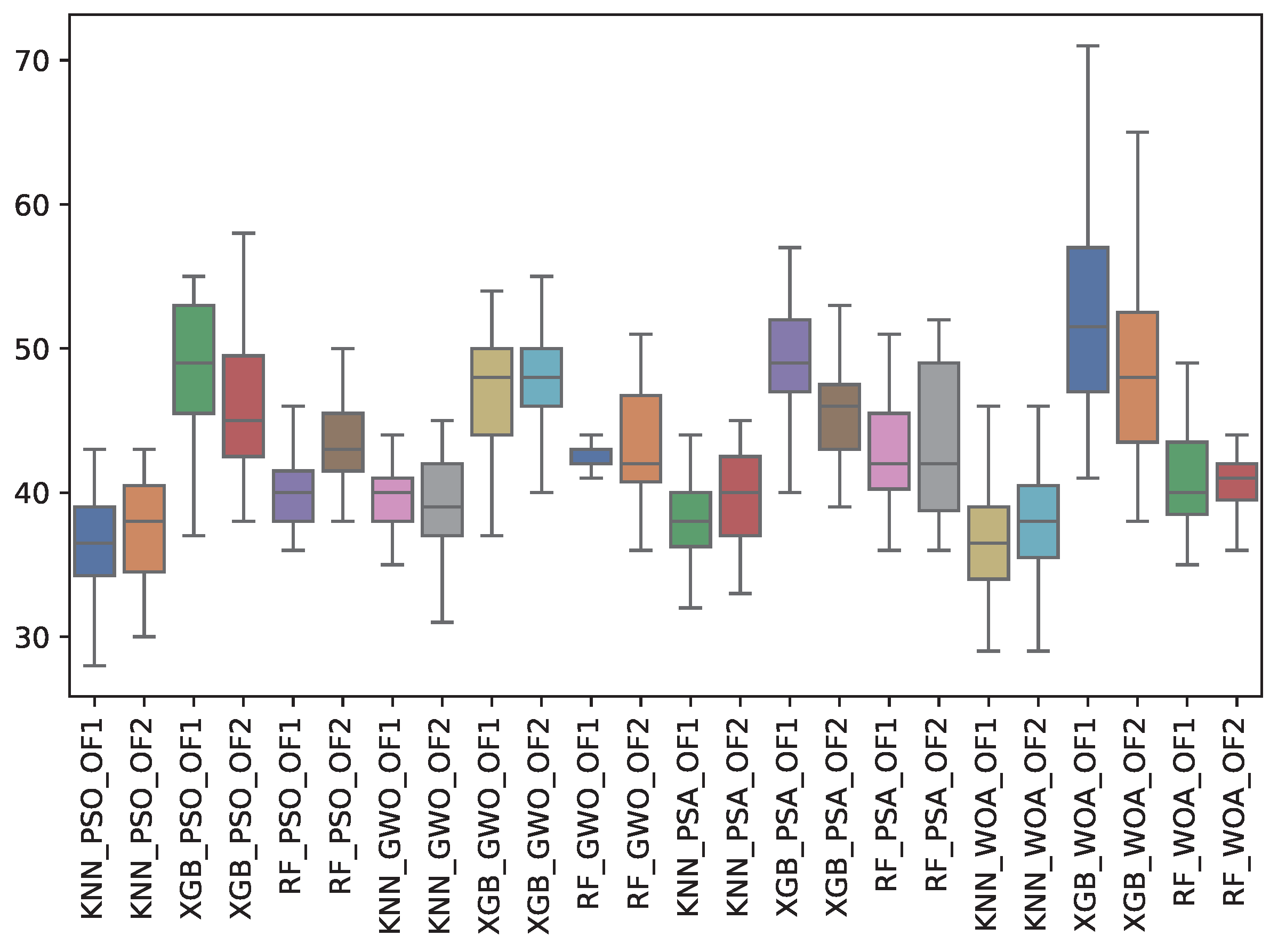
| TFS | Avg. | Std. | Avg. | Std. | Avg. | Std. | Avg. | Std. | Avg. | Std. | Avg. | Std. |
| GWO | 39.4 | 2.2 | 42.6 | 0.8 | 46.8 | 4.2 | 39.6 | 3.3 | 43.4 | 4.2 | 48.1 | 3.6 |
| PSA | 38.2 | 2.8 | 42.6 | 4.6 | 49.2 | 4.1 | 39.3 | 3.5 | 43.6 | 5.6 | 45.7 | 3.7 |
| PSO | 36.5 | 3.4 | 39.9 | 2.7 | 48.5 | 4.8 | 37.5 | 3.7 | 43.6 | 3.5 | 46.0 | 4.5 |
| WOA | 37.0 | 4.2 | 41.0 | 3.9 | 53.4 | 7.7 | 37.9 | 3.9 | 40.4 | 2.4 | 48.7 | 6.1 |
| OF1 | OF2 | |
|---|---|---|
| p-value |
| Algorithm | KNN_GWO | KNN_PSA | KNN_PSO | KNN_WOA | RF_GWO | RF_PSA | RF_PSO | RF_WOA | XGB_GWO | XGB_PSA | XGB_PSO | XGB_WOA |
|---|---|---|---|---|---|---|---|---|---|---|---|---|
| KNN_GWO | X | - | - | - | ||||||||
| KNN_PSA | - | X | - | - | ||||||||
| KNN_PSO | - | - | X | - | - | - | ||||||
| KNN_WOA | - | - | - | X | - | - | ||||||
| RF_GWO | - | - | X | - | - | - | - | |||||
| RF_PSA | - | - | - | X | - | - | - | |||||
| RF_PSO | - | - | X | - | - | - | - | - | ||||
| RF_WOA | - | - | - | X | - | - | - | - | ||||
| XGB_GWO | - | - | X | - | - | - | ||||||
| XGB_PSA | - | - | - | - | - | X | - | - | ||||
| XGB_PSO | - | - | - | - | X | - | ||||||
| XGB_WOA | - | - | - | - | - | X |
| Algorithm | KNN_GWO | KNN_PSA | KNN_PSO | KNN_WOA | RF_GWO | RF_PSA | RF_PSO | RF_WOA | XGB_GWO | XGB_PSA | XGB_PSO | XGB_WOA |
|---|---|---|---|---|---|---|---|---|---|---|---|---|
| KNN_GWO | X | - | - | - | ||||||||
| KNN_PSA | - | X | - | - | ||||||||
| KNN_PSO | - | - | X | - | - | - | - | - | ||||
| KNN_WOA | - | - | - | X | ||||||||
| RF_GWO | - | X | - | - | - | - | - | - | ||||
| RF_PSA | - | - | X | - | - | - | ||||||
| RF_PSO | - | - | - | X | - | - | ||||||
| RF_WOA | - | - | - | - | X | - | ||||||
| XGB_GWO | - | - | - | - | X | - | - | - | ||||
| XGB_PSA | - | - | X | - | - | |||||||
| XGB_PSO | - | - | X | - | ||||||||
| XGB_WOA | - | - | - | - | X |
| Algorithm | OF1 | OF2 |
|---|---|---|
| KNN_GWO | 0 | 0 |
| KNN_PSA | 0 | 0 |
| KNN_PSO | 0 | 0 |
| KNN_WOA | 0 | 0 |
| RF_GWO | 2 | 3 |
| RF_PSA | 2 | 3 |
| RF_PSO | 4 | 3 |
| RF_WOA | 4 | 3 |
| XGB_GWO | 6 | 4 |
| XGB_PSA | 4 | 7 |
| XGB_PSO | 6 | 8 |
| XGB_WOA | 6 | 7 |
| Comparison | p-Value | Conclusion |
|---|---|---|
| RF_GWO v/s KNN_GWO | 0.0 | RF_GWO is better than KNN_GWO |
| RF_GWO v/s KNN_PSA | 0.0 | RF_GWO is better than KNN_PSA |
| RF_PSA v/s KNN_GWO | 0.0 | RF_PSA is better than KNN_GWO |
| RF_PSA v/s KNN_PSA | 0.0 | RF_PSA is better than KNN_PSA |
| RF_PSO v/s KNN_GWO | 0.0 | RF_PSO is better than KNN_GWO |
| RF_PSO v/s KNN_PSA | 0.0 | RF_PSO is better than KNN_PSA |
| RF_PSO v/s KNN_PSO | 0.0 | RF_PSO is better than KNN_PSO |
| RF_PSO v/s KNN_WOA | 0.0 | RF_PSO is better than KNN_WOA |
| RF_WOA v/s KNN_GWO | 0.0 | RF_WOA is better than KNN_GWO |
| RF_WOA v/s KNN_PSA | 0.0 | RF_WOA is better than KNN_PSA |
| RF_WOA v/s KNN_PSO | 0.0 | RF_WOA is better than KNN_PSO |
| RF_WOA v/s KNN_WOA | 0.0 | RF_WOA is better than KNN_WOA |
| XGB_GWO v/s KNN_GWO | 0.0 | XGB_GWO is better than KNN_GWO |
| XGB_GWO v/s KNN_PSA | 0.0 | XGB_GWO is better than KNN_PSA |
| XGB_GWO v/s KNN_PSO | 0.0 | XGB_GWO is better than KNN_PSO |
| XGB_GWO v/s KNN_WOA | 0.0 | XGB_GWO is better than KNN_WOA |
| XGB_GWO v/s RF_GWO | 0.0001 | XGB_GWO is better than RF_GWO |
| XGB_GWO v/s RF_PSA | 0.0 | XGB_GWO is better than RF_PSA |
| XGB_PSA v/s KNN_GWO | 0.0 | XGB_PSA is better than KNN_GWO |
| XGB_PSA v/s KNN_PSA | 0.0 | XGB_PSA is better than KNN_PSA |
| XGB_PSA v/s KNN_PSO | 0.0 | XGB_PSA is better than KNN_PSO |
| XGB_PSA v/s KNN_WOA | 0.0 | XGB_PSA is better than KNN_WOA |
| XGB_PSO v/s KNN_GWO | 0.0 | XGB_PSO is better than KNN_GWO |
| XGB_PSO v/s KNN_PSA | 0.0 | XGB_PSO is better than KNN_PSA |
| XGB_PSO v/s KNN_PSO | 0.0 | XGB_PSO is better than KNN_PSO |
| XGB_PSO v/s KNN_WOA | 0.0 | XGB_PSO is better than KNN_WOA |
| XGB_PSO v/s RF_GWO | 0.0001 | XGB_PSO is better than RF_GWO |
| XGB_PSO v/s RF_PSA | 0.0001 | XGB_PSO is better than RF_PSA |
| XGB_WOA v/s KNN_GWO | 0.0 | XGB_WOA is better than KNN_GWO |
| XGB_WOA v/s KNN_PSA | 0.0 | XGB_WOA is better than KNN_PSA |
| XGB_WOA v/s KNN_PSO | 0.0 | XGB_WOA is better than KNN_PSO |
| XGB_WOA v/s KNN_WOA | 0.0 | XGB_WOA is better than KNN_WOA |
| XGB_WOA v/s RF_GWO | 0.0001 | XGB_WOA is better than RF_GWO |
| XGB_WOA v/s RF_PSA | 0.0 | XGB_WOA is better than RF_PSA |
| Comparison | p-Value | Conclusion |
|---|---|---|
| RF_GWO v/s KNN_GWO | 0.0001 | RF_GWO is better than KNN_GWO |
| RF_GWO v/s KNN_PSA | 0.0001 | RF_GWO is better than KNN_PSA |
| RF_GWO v/s KNN_WOA | 0.0001 | RF_GWO is better than KNN_WOA |
| RF_PSA v/s KNN_GWO | 0.0001 | RF_PSA is better than KNN_GWO |
| RF_PSA v/s KNN_PSA | 0.0001 | RF_PSA is better than KNN_PSA |
| RF_PSA v/s KNN_WOA | 0.0001 | RF_PSA is better than KNN_WOA |
| RF_PSO v/s KNN_GWO | 0.0001 | RF_PSO is better than KNN_GWO |
| RF_PSO v/s KNN_PSA | 0.0001 | RF_PSO is better than KNN_PSA |
| RF_PSO v/s KNN_WOA | 0.0001 | RF_PSO is better than KNN_WOA |
| RF_WOA v/s KNN_GWO | 0.0001 | RF_WOA is better than KNN_GWO |
| RF_WOA v/s KNN_PSA | 0.0001 | RF_WOA is better than KNN_PSA |
| RF_WOA v/s KNN_WOA | 0.0001 | RF_WOA is better than KNN_WOA |
| XGB_GWO v/s KNN_GWO | 0.0001 | XGB_GWO is better than KNN_GWO |
| XGB_GWO v/s KNN_PSA | 0.0001 | XGB_GWO is better than KNN_PSA |
| XGB_GWO v/s KNN_PSO | 0.0001 | XGB_GWO is better than KNN_PSO |
| XGB_GWO v/s KNN_WOA | 0.0001 | XGB_GWO is better than KNN_WOA |
| XGB_PSA v/s KNN_GWO | 0.0001 | XGB_PSA is better than KNN_GWO |
| XGB_PSA v/s KNN_PSA | 0.0001 | XGB_PSA is better than KNN_PSA |
| XGB_PSA v/s KNN_PSO | 0.0001 | XGB_PSA is better than KNN_PSO |
| XGB_PSA v/s KNN_WOA | 0.0001 | XGB_PSA is better than KNN_WOA |
| XGB_PSA v/s RF_PSA | 0.0001 | XGB_PSA is better than RF_PSA |
| XGB_PSA v/s RF_PSO | 0.0001 | XGB_PSA is better than RF_PSO |
| XGB_PSA v/s RF_WOA | 0.0001 | XGB_PSA is better than RF_WOA |
| XGB_PSO v/s KNN_GWO | 0.0001 | XGB_PSO is better than KNN_GWO |
| XGB_PSO v/s KNN_PSA | 0.0001 | XGB_PSO is better than KNN_PSA |
| XGB_PSO v/s KNN_PSO | 0.0001 | XGB_PSO is better than KNN_PSO |
| XGB_PSO v/s KNN_WOA | 0.0001 | XGB_PSO is better than KNN_WOA |
| XGB_PSO v/s RF_GWO | 0.0001 | XGB_PSO is better than RF_GWO |
| XGB_PSO v/s RF_PSA | 0.0001 | XGB_PSO is better than RF_PSA |
| XGB_PSO v/s RF_PSO | 0.0001 | XGB_PSO is better than RF_PSO |
| XGB_PSO v/s RF_WOA | 0.0001 | XGB_PSO is better than RF_WOA |
| XGB_WOA v/s KNN_GWO | 0.0001 | XGB_WOA is better than KNN_GWO |
| XGB_WOA v/s KNN_PSA | 0.0001 | XGB_WOA is better than KNN_PSA |
| XGB_WOA v/s KNN_PSO | 0.0001 | XGB_WOA is better than KNN_PSO |
| XGB_WOA v/s KNN_WOA | 0.0001 | XGB_WOA is better than KNN_WOA |
| XGB_WOA v/s RF_PSA | 0.0001 | XGB_WOA is better than RF_PSA |
| XGB_WOA v/s RF_PSO | 0.0001 | XGB_WOA is better than RF_PSO |
| XGB_WOA v/s RF_WOA | 0.0001 | XGB_WOA is better than RF_WOA |
Disclaimer/Publisher’s Note: The statements, opinions and data contained in all publications are solely those of the individual author(s) and contributor(s) and not of MDPI and/or the editor(s). MDPI and/or the editor(s) disclaim responsibility for any injury to people or property resulting from any ideas, methods, instructions or products referred to in the content. |
© 2025 by the authors. Licensee MDPI, Basel, Switzerland. This article is an open access article distributed under the terms and conditions of the Creative Commons Attribution (CC BY) license (https://creativecommons.org/licenses/by/4.0/).
Share and Cite
Cisternas-Caneo, F.; Santamera-Lastras, M.; Barrera-Garcia, J.; Crawford, B.; Soto, R.; Brante-Aguilera, C.; Garcés-Jiménez, A.; Rodriguez-Puyol, D.; Gómez-Pulido, J.M. Application of Metaheuristics for Optimizing Predictive Models in iHealth: A Case Study on Hypotension Prediction in Dialysis Patients. Biomimetics 2025, 10, 314. https://doi.org/10.3390/biomimetics10050314
Cisternas-Caneo F, Santamera-Lastras M, Barrera-Garcia J, Crawford B, Soto R, Brante-Aguilera C, Garcés-Jiménez A, Rodriguez-Puyol D, Gómez-Pulido JM. Application of Metaheuristics for Optimizing Predictive Models in iHealth: A Case Study on Hypotension Prediction in Dialysis Patients. Biomimetics. 2025; 10(5):314. https://doi.org/10.3390/biomimetics10050314
Chicago/Turabian StyleCisternas-Caneo, Felipe, María Santamera-Lastras, José Barrera-Garcia, Broderick Crawford, Ricardo Soto, Cristóbal Brante-Aguilera, Alberto Garcés-Jiménez, Diego Rodriguez-Puyol, and José Manuel Gómez-Pulido. 2025. "Application of Metaheuristics for Optimizing Predictive Models in iHealth: A Case Study on Hypotension Prediction in Dialysis Patients" Biomimetics 10, no. 5: 314. https://doi.org/10.3390/biomimetics10050314
APA StyleCisternas-Caneo, F., Santamera-Lastras, M., Barrera-Garcia, J., Crawford, B., Soto, R., Brante-Aguilera, C., Garcés-Jiménez, A., Rodriguez-Puyol, D., & Gómez-Pulido, J. M. (2025). Application of Metaheuristics for Optimizing Predictive Models in iHealth: A Case Study on Hypotension Prediction in Dialysis Patients. Biomimetics, 10(5), 314. https://doi.org/10.3390/biomimetics10050314