2.2. Mathematical Modeling of ESC
(1) Initialization
Using random initialization in ESC,
In the formula, represent the lower and upper bounds of the th dimension, the value of the random variable follows a uniform distribution between 0 and 1.
Then, calculate the fitness values of the population and arrange them in ascending order. Store the optimal individuals in the elite pool
Epool, where these elites are the best possible solutions that have been discovered, The specific expression is as follows:
(2) Panic index
This value represents the panic level of the crowd during the evacuation process, expressed as follows:
The larger the value, the more chaotic the behavior becomes. As the iteration progresses, the panic level decreases and the crowd gradually adapts to the environment. In the equation, represents the current iteration count and represents the maximum iteration count.
(3) Exploration stage
The three states of calmness, gathering, and panic are grouped according to the ratio, which is in line with the actual behavioral state of the crowd in emergency situations. Most people are in a state of panic, and only a small number of people are calm.
Calm down group update:
in the formula,
represents the mean of all calm groups in the
th dimension,
is obtained according to the following equation,
In the formula, represents the group position of the calm group, represents the maximum and minimum values of the calm group in the th dimension, respectively, represents the individual’s adjustment value that satisfies , is a random value of 0 or 1, and is the adaptive Levy weight.
Aggregation group update:
In the equation,
is a random individual within the panic group, and the vector
is obtained according to the following equation,
In the formula, is a random position, is the maximum and minimum values of the cooling group, and is similar to .
Panic Group Update:
The impact of random indications on the fertilization pool of individuals in the panic group and other individuals,
In the formula,
represents individuals in the elite pool,
represents randomly selected individuals in the population, and the vector
is obtained according to the following equation,
In the formula, is the group position of the panic group, and is the upper and lower bounds of the panic group.
(4) Development stage
At this stage, all individuals remain calm and improve their position by approaching members of the elite pool. This process simulates the crowd gradually gathering towards the determined optimal exit,
In the formula, represents the individual’s position, and represents the currently obtained best solution or exit.
2.3. The Proposed mESC Algorithm
ESC performs well in solving simple problems in low dimensions, but its performance significantly decreases when solving complex multimodal and combinatorial functions. This means that it is more prone to getting stuck in local solution spaces, and the continuous reduction in population diversity makes it difficult for the algorithm to maintain synchronous exploration and development, ultimately leading to overall performance degradation. Therefore, this article proposes some improvement strategies and develops the mESC algorithm to address these shortcomings. The specific improvement strategies are as follows.
2.3.1. Adaptive Perturbation Factor Strategy
Generally speaking, the population diversity of algorithms will decrease as the algorithm runs, and the significant reduction in diversity in the later stages of iteration is not conducive to the full exploration of the population. This article proposes an adaptive perturbation factor to overcome this drawback, which adjusts the perturbation probability of individuals in the population as the iteration progresses; furthermore, it enriches the diversity of the population. The specific expression is as follows:
is a random number in the equation.
As increases, it enhances the global search capability and avoids falling into local optima. However, as gradually decreases, it improves the local search accuracy and accelerates convergence. For continuous functions, when an individual has not yet found the optimal solution, there are better solutions nearby. The adaptive perturbation factor can adjust the individual extremum, global extremum, and position term to increase the possibility of finding the global optimal solution.
2.3.2. Restart Mechanism
ESC has the drawbacks of premature stagnation and getting stuck in local space, and this article uses a restart mechanism [
29] to improve this. This mechanism can enhance the robustness of ESC while improving the global search capability, and effectively eliminating some poor individuals, thereby achieving the goal of enhancing algorithm convergence.
We set the worst individual factor in this article to 0.05, select the worst quantity as
, and
as the population size. The position update equation for these worst individuals is as follows:
satisfies the formula in the equation,
In the formula, follows a Gaussian distribution, represents the optimal individual, and is a random number.
In this strategy, the restart mechanism gives the algorithm the opportunity to jump out of local optima and explore other solution spaces, thereby increasing the probability of finding the global optimum. In addition, as the iteration progresses, the convergence speed may slow down. However, the restart mechanism is equivalent to using the fast convergence characteristics of the population in the initial stage of the iteration, and this mechanism can prompt the algorithm to continue optimization when facing local stagnation.
2.3.3. Boundary Adjustment Strategy Based on Elite Pool
According to Equation (10), we have obtained the position of the entire population. Next, we will perform boundary processing on the obtained positions to ensure the correctness and robustness of the algorithm by applying specific processing methods to the boundaries or extreme cases. Generally, when an individual exceeds the population boundary, they are indiscriminately assigned a critical value to the boundary, which can lead to local aggregation of individuals on the boundary and affect the search for the global optimal solution. This article introduces the boundary adjustment strategy of the elite pool, which updates the boundaries of individuals in the population based on the selected members in the elite pool.
Therefore, the position formula of the population is updated to,
In the formula, .
In this strategy, the elite pool ensures that the optimal solutions of each iteration are not eliminated by storing them, and these elite solutions reduce invalid searches by concentrating on the search potential area. By retaining diverse elite solutions, it is possible to prevent the population from prematurely falling into local solutions and enhance global search capabilities. Because elite solutions come from different regions of the population, this can maintain a balance between exploration and development for the algorithm. After mastering the position of the elite solution, the boundary can be adjusted to search in the area that is most likely to find the global optimal solution.
2.3.4. Dynamic Centroid Reverse Learning Strategy
This article proposes a random centroid reverse learning strategy to improve ESC. Based on the idea of reverse learning, while considering existing solutions, opposite solutions are also taken into account. By comparing with the reverse solution, choose the better solution to guide other individuals in the population to seek optimization. While balancing the concepts of adversarial learning and centroids, the robustness of mESC is improved by introducing randomness elements, in the following specific form:
Generate integer
, which is the number of randomly selected populations. Then, randomly select
individuals from the current population and calculate their centroids, expressed as follows:
Then, generate the population’s ortho solutions about the centroid, as shown below:
Finally, using the greedy rule, the top individuals with the best fitness values were selected from the original improved population and the population that underwent random centroid reverse learning as the new generation population. The random centroid reverse learning strategy utilizes the excellent solutions obtained from the previous generation to guide population initialization, improve algorithm accuracy, accelerate convergence speed, and enable faster search near potentially optimal positions.
In this strategy, the centroid will dynamically update with changes in the population to ensure that the algorithm can respond to changes in the population in a timely manner to avoid premature convergence. After integrating reverse learning, the reverse solution expands the search space and increases the diversity of the population, which helps to escape from local optima
2.3.5. Specific Steps of mESC
The pseudocode of the improved escape algorithm incorporating adaptive perturbation factor, restart mechanism, boundary adjustment strategy based on elite pool, and dynamic centroid reverse learning strategy, is listed in Algorithm 1.
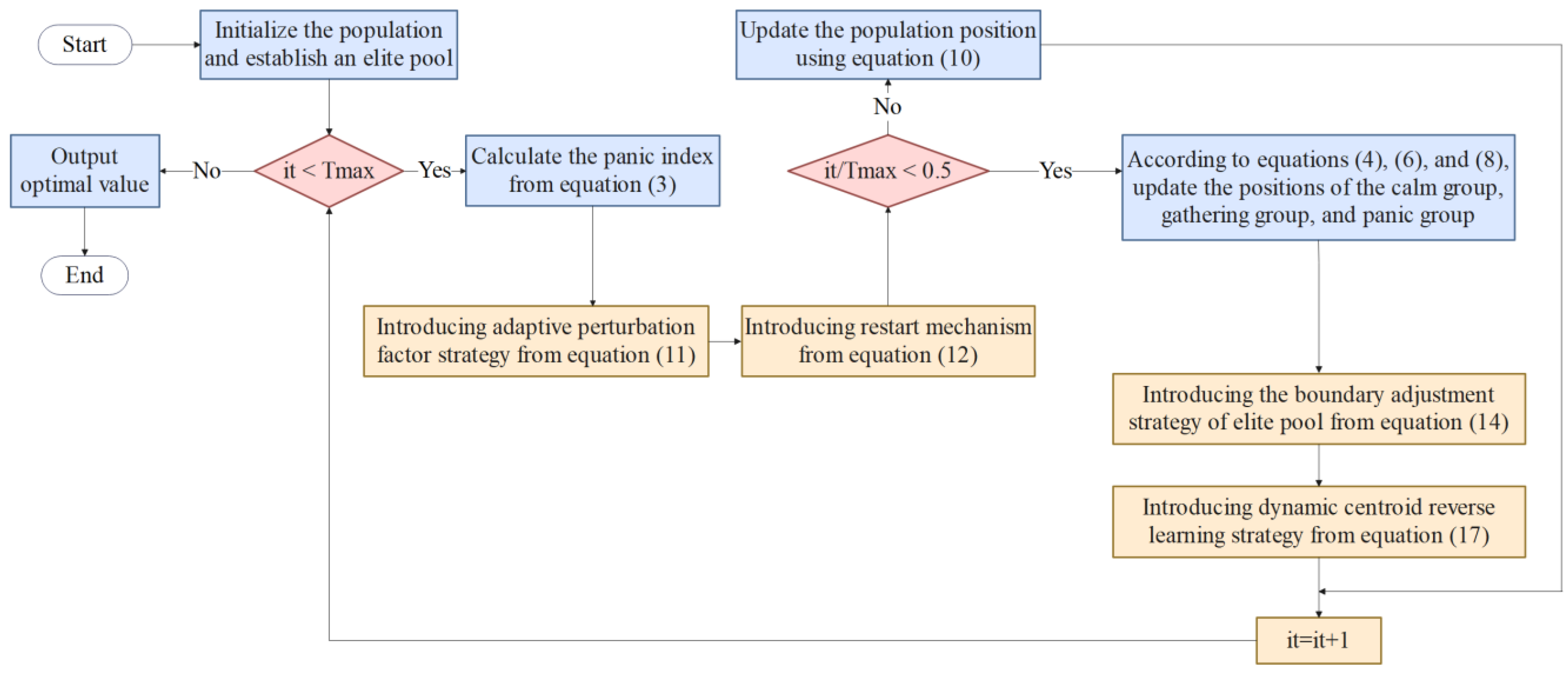
Figure 1 shows the flowchart of mESC.
| Algorithm 1 The proposed mESC |
| Input: Dimension , Population , Population size , Maximum number of iterations , The worst individual ratio Pworst is 0.1 |
| Output: Optimal fitness value |
| 1: Randomly initialize the individual positions of the population using Equation (1) |
| 2: Sort the fitness values of the population in ascending order and record the current optimal individual |
| 3: Store the refined individuals in the elite pool of Equation (2) |
| 4: while do |
| 5: Calculate the panic index from Equation (3) |
| 6: |
| 7: for do |
| 8: for do |
| 9: |
| 10: |
| 11: end for |
| 12: end for |
| 13: if then |
| 14: Divide the population into three groups and update the three groups according to Equations (4), (6) and (8) |
| 15: else |
| 16: Equation (10) updates the population |
| 17: end |
| 18: for do |
| 19: |
| 20: |
| 21: end |
| 22: |
| 23: Calculate individual fitness values and update the elite pool based on the optimal value |
| 24: |
| 25: end while |
| 26: Return the optimal solution from the elite pool |
2.5. Experimental Setup
We conducted two sets of comparative experiments to validate the performance of the proposed algorithm. The first set compared mESC with 16 other newly proposed metaheuristic algorithms, including some competitive algorithms proposed in 2023 and 2024, which showed excellent performance in solving some problems. The second group conducted comparative experiments between mESC and 11 high-performance, winner algorithms, including 3 winner algorithms from CEC competitions, 4 variant algorithms from DE, and 3 variant algorithms from PSO. These algorithms have generally strong performance and are often used as competitors in comparative experiments. By comparing with current new algorithms and powerful algorithms in the past, the superiority of mESC is highlighted.
This article will include some experimental tables and images in the
Supplementary Materials. Among them,
Tables S1 and S2 and Tables S3 and S4, respectively, show the results of two types of parameters in the 10 and 20 dimensions.
Tables S5 and S6 and Tables S7 and S8 show the experimental results and Wilcoxon results of mESC and the novel metaheuristic algorithm in 10 and 20 dimensions, respectively.
Tables S9 and S14 show the running times of mESC, the new metaheuristic algorithm, and the high-performance, winner algorithm, respectively.
Tables S10 and S11 and
Tables S12 and S13, respectively, show the experimental results and Wilcoxon results of mESC and high-performance, winner algorithm in 10 and 20 dimensions.
Figures S1 and S2 show the convergence curves and boxplots of mESC and the novel metaheuristic algorithm, respectively.
Figures S3 and S4 show the convergence curves and boxplots of mESC and high-performance, winner’s algorithm, respectively.
2.5.1. Benchmark Test Function
Use the CEC2022 (D = 10, 20) test kit to evaluate the performance of mESC for two comparative experiments. Set the population size of mESC to 30, with a maximum iteration of 500, and run it independently 30 times as a whole.
2.5.2. Parameter Settings
The new metaheuristic algorithms compared in the first set of experiments include Parrot Optimization (PO) [
30], Geometric Mean Optimization (GMO) [
31], Fata Morgana Algorithm (FATA) [
32], Moss Growth Optimization (MGO) [
33], Crown Pig Optimization (CPO) [
34], Polar Lights Optimization (PLO) [
35], Newton–Raphson-based Optimizer (NRBO) [
36], Information Acquisition Optimization (IAO) [
37], Love Evolutionary Algorithm (LEA) [
38], Escape Algorithm (ESC), Improved Artificial Rabbit Optimization (MNEARO), Artificial Hummingbird Algorithm (AHA), Dwarf Mongoose Optimization Algorithm (DMOA), Zebra Optimization Algorithm (ZOA), and Seahorse Optimization (SHO). The high performance compared in the second set of experiments, the winning algorithm includes Autonomous Particle Groups for Particle Dwarm Optimization (AGPSO) [
39], Integrating Particle Swarm Optimization and Gravity Search Algorithm (CPSOGSA) [
40], Improved Particle Swarm Optimization (TACPSO) [
41], Bernstein–Levy Differential Evolution (BDE) [
42], Bezier Search Differential Evolution (BeSD) [
43], Multi Population Differential Evolution (MDE) [
44], Improving Differential Evolution through Bayesian Hyperparameter Optimization (MadDE) [
45], Improved LSHADE Algorithm (LSHADE-cnEpSin) [
46], Improvement of L-SHADE Using Semi-parametric Adaptive Method (LSHADE-SPACMA) [
47], and Improving SHADE with Linear Population Size Reduction (LSHADE) [
48]. All parameters are given in
Table 1.
2.5.3. Empirical Test
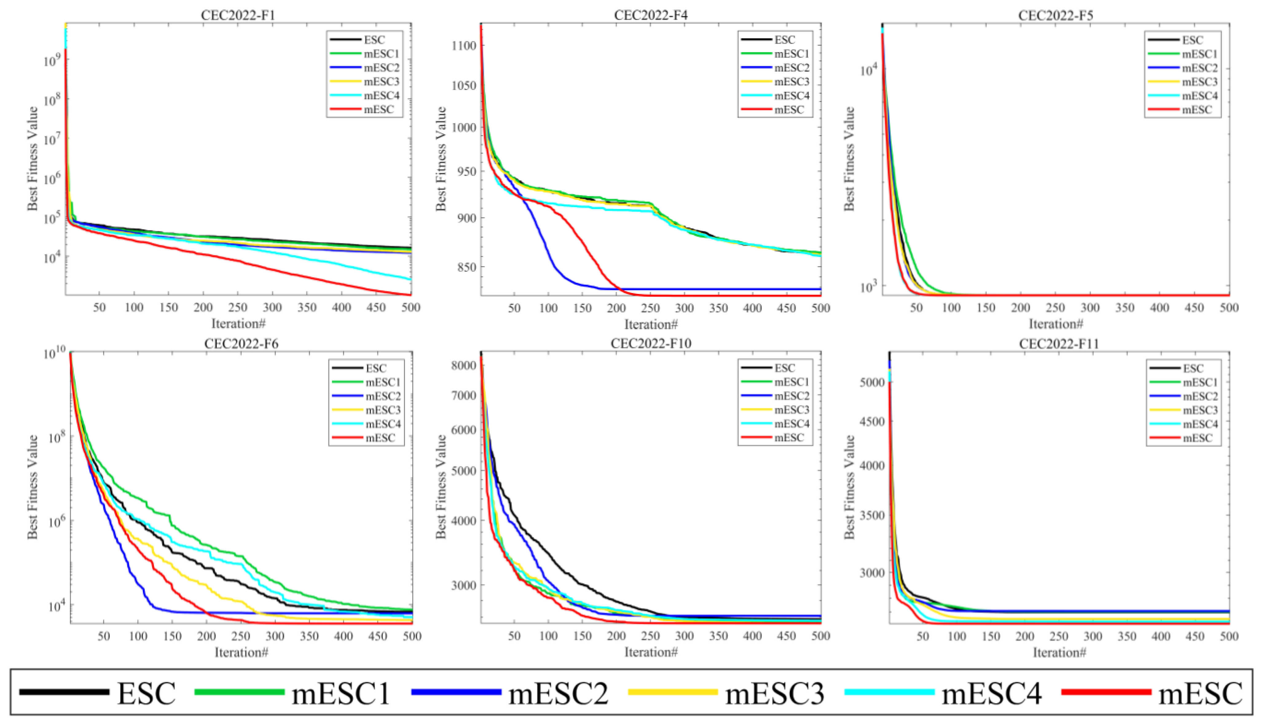
Before starting this section, we defined mESC1, mESC2, mESC3, and mESC4 as algorithms that separately introduce adaptive perturbation factors, restart mechanisms, boundary adjustment strategies based on elite pools, and dynamic centroid reverse learning strategies for mESC. Subsequently, we conducted impact analysis on mESC, ESC, mESC1, mESC2, mESC3, and mESC4, and discussed the degree of impact of the proposed individual strategies on the original ESC and mESC.
Given the convergence of six algorithms from
Figure 2, when solving the F1 problem, mESC and mESC4 have the best convergence effect, while other competitors have all fallen into local optima after a mid-term operation. However, mESC has a convergence effect that is 1 or 2 orders of magnitude better than mESC4. For F4, mESC and mESC2 have the closest convergence effects. For F5, visually speaking, the convergence of the six algorithms is very close, but mESC has the fastest convergence speed. For F6, mESC has the highest convergence accuracy, while mESC2 converges faster than mESC. For F10, mESC1, mESC3, mESC4, and mESC, their convergence is very close at the beginning of the operation, but mESC has a higher convergence accuracy. The convergence of F11, mESC, and mESC4 are very similar, while the convergence accuracy of other algorithms is inferior to mESC. The four strategies play different roles in improving the algorithm, which is related to their different mechanisms, and combining them will produce better results.
Table 2 presents the 12 experimental results on the CEC2022 test suite, and according to this table, mESC has the best overall performance. MESC has the optimal mean on 10 questions and the optimal standard deviation on four questions, indicating that the combination of these four improvement strategies is effective. MESC is optimal on unimodal functions and can also achieve optimality on fundamental functions. The performance of mESC3 is optimal on the mixed function F6, while mESC reaches its optimum on F7 and F8. MESC1 performs the best on F10, outperforming mESC, while mESC performs better on other functions. Overall, we can demonstrate that mESC performs the best and validates the effectiveness of the four strategies.
2.5.4. Sensitivity of the Parameters
In the proposed mESC, the main strategies introduced are the proportion of worst-performing individuals
in the restart mechanism and the parameter adaptive disturbance factor adjustment range
in the adaptive disturbance factor strategy, which affect the performance of the algorithm. In this section, we determine the relevant parameters on the CEC2022 test set. The variable dimensions in the experiment are the standard dimensions 10 and 20 of the test set, with a maximum iteration of 500. The average values obtained from different parameters are shown in
Tables S1–S4 and the ranking is given in the last row of the table.
The worst individual ratio
determines the proportion of individuals replaced after each restart. A smaller value will make it easier to fall into local optima while accelerating convergence, while a larger value will significantly slow down convergence while making global search stronger. The parameter ranges from 0.05 to 0.20 and increases by 0.05. As shown in
Tables S1 and S2,
achieves better performance and performance in both 10 and 20 dimensions based on the final ranking.
The adaptive interference factor adjustment range
determines the variation range of the interference factor. When the problem to be solved requires a high convergence speed, this range can be appropriately reduced. However, for scenarios with high solution quality, the variation range should be increased. In
Tables S3 and S4, values are selected between 0.9 and 0.5 in increments gradually decreasing by 0.01. The results indicate that the most promising range is when the parameter decreases between 0.7 and 0.5.
2.6. Experimental Analysis of mESC and New Metaheuristic Algorithm
As shown in
Figure S1, mESC has good convergence performance compared to other competitors when dealing with different dimensional problems on CEC2022. Given MESC in F1 on the 10 dimensions, F3, F5, F7, the convergence speed in the early stage is the fastest, and it can quickly find the global optimum. ZOA has the fastest convergence speed in the early stage on F4, while LEA and CPO fall into local optima prematurely on multiple functions. The optimization accuracy of mESC is much better than other algorithms. On the 20-dimensional F4 problem, ZOA, SHO, and NRBO converge slightly faster than the proposed algorithm in the early stages of iteration, but mESC has the best convergence accuracy. On F3, F4, and F11, AHA, MNEARO, ESC, and mESC have very similar convergence accuracy in the middle and later stages of iteration, but mESC has higher convergence accuracy.
From
Tables S5 and S6, it can be seen that mESC’s overall average ranking and ranking on various benchmark functions are superior to other competitors, demonstrating superior performance. The overall ranking in 10 dimensions is 1.83, ranking first on 5 benchmark functions. MNEARO’s overall ranking is second only to mESC. The overall ranking in 20 dimensions is 1.50, ranking first on 8 benchmark functions, while MGO ranks worst in two dimensions.
Tables S7 and S8 present the statistical results of the Wilcoxon rank sum test on different dimensions of CEC2022. On the 10 dimensions, mESC outperforms PO, FATA, MGO, ECO, CPO, PLO, NRBO, LEA, SHO, ZOA, and MNEARO on all 12 benchmark functions. On the 20 dimensions, mESC outperforms PO, FATA, MGO, NRBO, ECO, CPO, PLO, LEA, SHO, ZOA, and MNEARO on 12 benchmark functions, and also outperforms mESC on five functions.
Figure S2 shows the boxplots of mESC and other competitors in different dimensions of CEC2022. Overall, mESC has shorter boxes on different functions, especially F1, F3, F5, and F7 on the 10 dimensions and F2 on the 20 dimensions, F9, F10, and F11, This demonstrates the superiority and stability of mESC.
The running time of an algorithm is also an indicator for evaluating its performance. As shown in
Table S9, CPO has the shortest running time and ranks first, while mESC ranks very low in both dimensions of running time, which is in line with our expectations. Because it is inevitable that the algorithm will run for too long while ensuring its performance, we allow this phenomenon to occur.
2.7. Experimental Analysis of mESC and High-Performance, Winner Algorithm
The experimental results of mESC and high-performance, winner algorithm on CEC2022 are presented in
Tables S10 and S11. On the 10 dimensions, mESC outperforms other competitors on 8 benchmark functions, ranking first overall with an average ranking of 1.58. MadDE, ranked second overall, outperforms the proposed algorithm on two benchmark functions with an average ranking of 3.50. MDE performs better than mESC on two benchmark functions, but its overall ranking is only fourth. Overall, mESC’s testing with these competitors has validated its superior performance.
Tables S12 and S13 show the Wilcoxon rank sum test of mESC and high-performance, winner algorithm on the CEC2022 test suite (symbol ♢ = 3.0199 × 10
−11 in the table). On the 10 dimensions, BDE, BeSD, MDE, and MadDE have better
p-values than mESC on 2, 2, 2, and 3 benchmark functions, respectively. The
p-values of mESC on 12 functions are completely superior to AGPSO, TACPSO, LSAHDE cnEpSin, and LSHADE. On the 20 dimensions, mESC outperforms the other seven competitors on 12 benchmark functions and only has approximate performance on one function compared to CPSOGSA, TACPSO, and MDE. Therefore, we can say that the proposed strategy significantly improves the algorithm.
Figure S3 shows the convergence curve of mESC and high-performance, winner algorithm on CEC2022. In terms of 10 dimensions, the convergence of mESC is superior to other competitors. LSAHDE-SPACMA, LSAHDE, and CPSOGSA began to fall into local optima in the mid-iteration of F1 and F4. On the 20th dimension, as the dimension increases, the convergence speed of mESC improves. The accuracy of mESC on F1 and F4 is significantly better than other competitors, and some algorithms fall into local optima early on F3, F7, and F11 while mESC can maintain stability for optimization.
Table S14 presents the comparison results of the running time between mESC and high-performance, winner algorithms. The running time ranking of mESC is 12th in both dimensions, which is in line with our initial expectations. LSHADE has the shortest running time and ranks first.
Figure S4 shows the boxplots of mESC and other algorithms in different dimensions of CEC2022. Overall, mESC has shorter boxes for the vast majority of functions, especially F1, F5, F7, F1 in the 10 dimensions, and F1 in the 20 dimensions, F2, F4, F8. This indicates the stability of mESC.


