Article

Exploring the Robustness of Alternative Cluster Detection and the Threshold Distance Method for Crash Hot Spot Analysis: A Study on Vulnerable Road Users

Department of Transportation, Logistics and Finance, College of Business, North Dakota State University, P.O. Box 6050, Fargo, ND 58108-6050, USA
*
Author to whom correspondence should be addressed.
Safety 2023, 9(3), 57; https://doi.org/10.3390/safety9030057
Submission received: 6 June 2023 / Revised: 18 August 2023 / Accepted: 23 August 2023 / Published: 25 August 2023

Abstract

:
Traditional hot spot and cluster analysis techniques based on the Euclidean distance may not be adequate for assessing high-risk locations related to crashes. This is because crashes occur on transportation networks where the spatial distance is network-based. Therefore, this research aims to conduct spatial analysis to identify clusters of high- and low-risk crash locations. Using vulnerable road users’ crash data of San Francisco, the first step in the workflow involves using Ripley’s K-and G-functions to detect the presence of clustering patterns and to identify their threshold distance. Next, the threshold distance is incorporated into the Getis-Ord Gi* method to identify local hot and cold spots. The analysis demonstrates that the network-constrained G-function can effectively define the appropriate threshold distances for spatial correlation analysis. This workflow can serve as an analytical template to aid planners in improving their threshold distance selection for hot spot analysis as it employs actual road-network distances to produce more accurate results, which is especially relevant when assessing discrete-data phenomena such as crashes.

1. Introduction

Vulnerable road users include pedestrians, bicyclists, and some small motorized (2-wheeler and 3-wheeler) vehicles. The proportion of crashes involving vulnerable road users in the United States is approximately 34%, and they mostly occur in urban areas [1]. Among pedestrians, children, the elderly, and people with impairments or disabilities are most commonly involved in crashes [2]. The most common spatial analysis methods used by researchers to find crash clusters in road networks are Moran’s Index (also known as Moran’s I), Getis-Ord Gi*, Kernel Density Estimation, and Ripley’s K-function [2,3,4]. Patrick Moran introduced the concept of spatial autocorrelation in 1948 and modified it in 1950, which measures multi-dimensional autocorrelation and clustering in space through Moran’s Index [5,6]. In 1976 and 1977, another scientist, Dr. Brian Ripley, introduced another method (Ripley’s K-function) for the identification of spatial patterns of points in space [7]. Later, in 1992, Getis and Ord introduced Getis-Ord Gi* statistics for the study of local patterns in spatial data, and in 1995, modifications were made to the method, and spatial weights were introduced to identify a correlation between nearby spatial data points [8,9]. In 1993 and 1995, Luc Anselin further contributed to the field by introducing the Local Indicator of Spatial Association (LISA), which measures the local spatial association and differs from Getis-Ord Gi* statistics [10]. Kernel density estimation evolved over the period of decades, whereas its foundation was laid by Rosenblatt in the 1950s. Moran’s Index requires testing a null hypothesis of spatial randomness [6]. The method can use Monte Carlo simulations to randomly distribute points on the network to conduct the test. Moran’s Index and Getis-Ord Gi* methods tend to provide better results than the K-function, but they are more sensitive to the selection bias of threshold distances for spatial analysis [11]. The threshold distance is a cutoff distance used to define the scale of analysis to reveal spatial autocorrelation [12]; therefore, choosing an appropriate threshold distance is particularly important because different scales of analysis can lead to different results and conclusions. Finding crash clusters is crucial in order to proactively address road safety issues and use data-based strategies to reduce crash injury severity and frequencies.
Most spatial analysis methods use an Euclidean distance between events to estimate their spatial dependence based on the notion that events closer together are more similar than events farther apart [13]. The main limitation of such methods is that they cannot account for the actual travel distance constrained by the road network [14,15]. There is no agreed best method to select the threshold distance for estimating spatial dependence [12]. The threshold distance used to estimate spatial autocorrelation plays a key role in identifying clusters. Using Euclidean distances for weighted matrices rather than network distances may incorrectly show clustering when one does not exist, and vice versa [16,17,18,19,20,21,22,23,24,25]. Figure 1 illustrates a scenario that further explains the reason for the differences in threshold distances. The scenario is that one crash occurred on a bridge crossing a highway and the other occurred under the bridge on the highway. The illustration shows that the Euclidean distance is much shorter than the network-constrained distance. This scenario highlights why using network-constrained distances would provide more accurate results in crash cluster analysis, which also agrees with the previous findings [15].
Other studies have used incremental spatial autocorrelation with Moran’s Index to find an appropriate threshold distance using Euclidean distance measurements; however, they later used networked constrained spatial autocorrelation to identify hot spots [18,19]. It is evident from the literature that the researchers either did not discuss a method of threshold distance selection [21,26], assumed a threshold distance [11,27], or searched for a threshold distance by performing incremental spatial autocorrelation using Moran’s I analysis [19,28].
The objective of this research is to propose the use of an alternate method based on network-constrained point pattern analysis. This is in contrast to the typically used method based on the Euclidean distance for finding the threshold distance for hot spot analysis and to evaluate the prediction accuracy by comparing the results with the outcome of the methods that have already been used by researchers. In this study, we hypothesize that network-constrained point pattern analysis will yield different threshold distances for crash hot spots compared to the conventional Euclidean distance method, and the predictions from the alternate method will demonstrate comparable accuracy when evaluated against the established techniques. These results aim to address the question: Can network-constrained point pattern analysis accurately identify crash hot spots comparable to Euclidean methods?
The implication is that decision-makers may not have the best information to make optimal decisions toward crash mitigation. To the best of our knowledge, researchers have not used Ripley’s G- and K-functions with network-constrained distances to account for actual travel distances in crash hot spot analysis. We fill this gap with the following contributions:
  • Developed a framework of an alternate method to identify the clustering strength and threshold distance for network-constrained hot spot analysis.
  • Demonstrated the use of the cross-K- and cross-G-functions to select the best crash hot spots among different outcomes.
It should be noted that the G-function and K-function are point pattern analyses and do not take any quantitative values for calculation, whereas Global Moran’s Index takes a quantitative value for calculation, which is injury severity level in this study. To overcome this limitation, we used Getis-Ord Gi* statistics after the G-/K-functions and after Global Moran’s Index analysis. The framework of the proposed methodology can be used for any kind of crash data. According to the research note published by the National Highway Traffic Safety Administration (NHTSA), over the last decade, a gradual increase in the proportion of Vulnerable Road Users (VRU) annual fatal crashes was observed and reached a high of 34% of total fatal crashes in 2019 in the U.S. [1]. In this study, we used the crash data of Vulnerable Road Users (VRU), specifically bicyclists and pedestrians, from the city of San Francisco, which are readily available.
The organization of the rest of this paper is as follows: Section 2 presents a literature review of related works. The methodology used in this study is explained in Section 3. The results are discussed in Section 4, and Section 5 presents the conclusions.

2. Literature Review
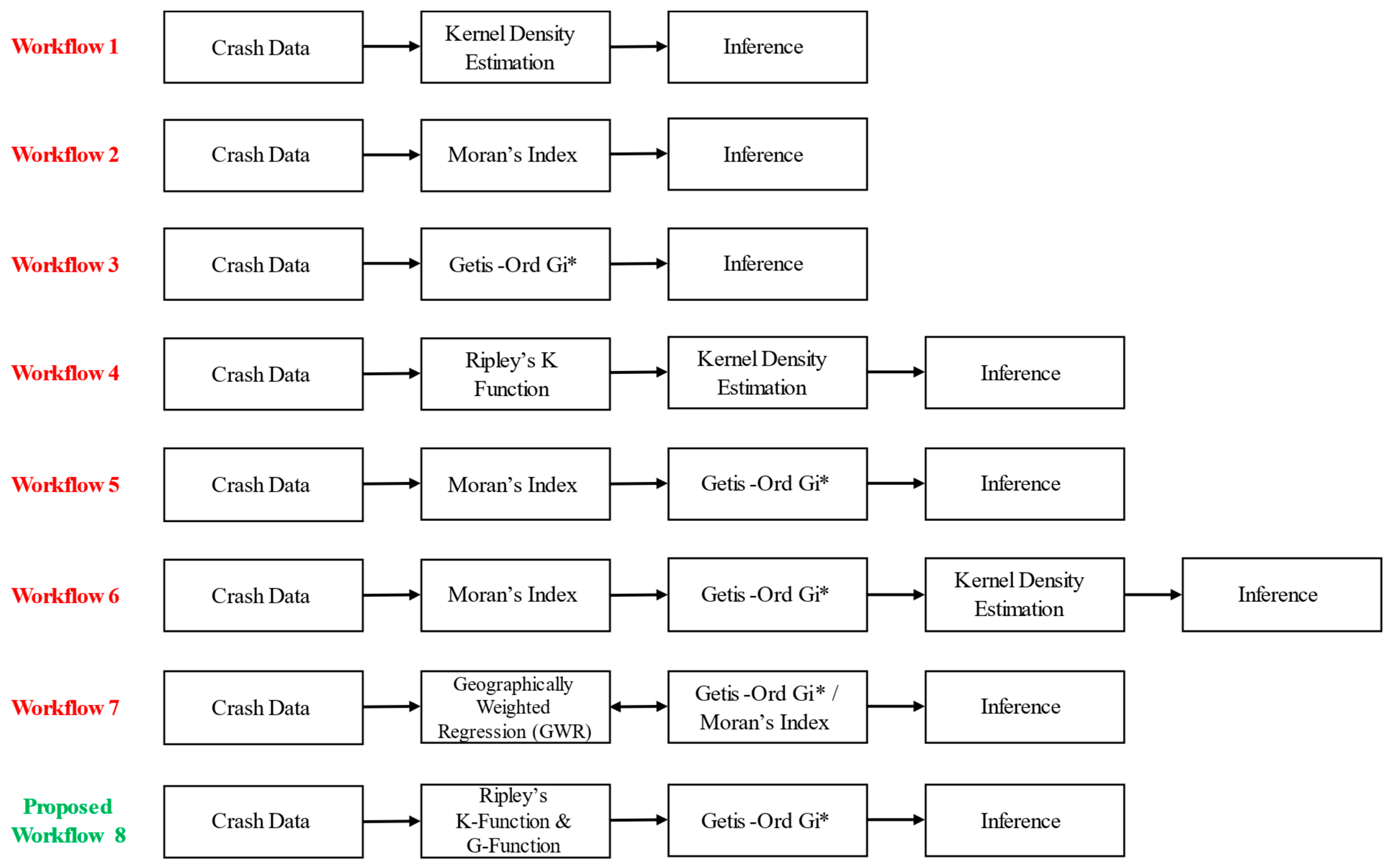
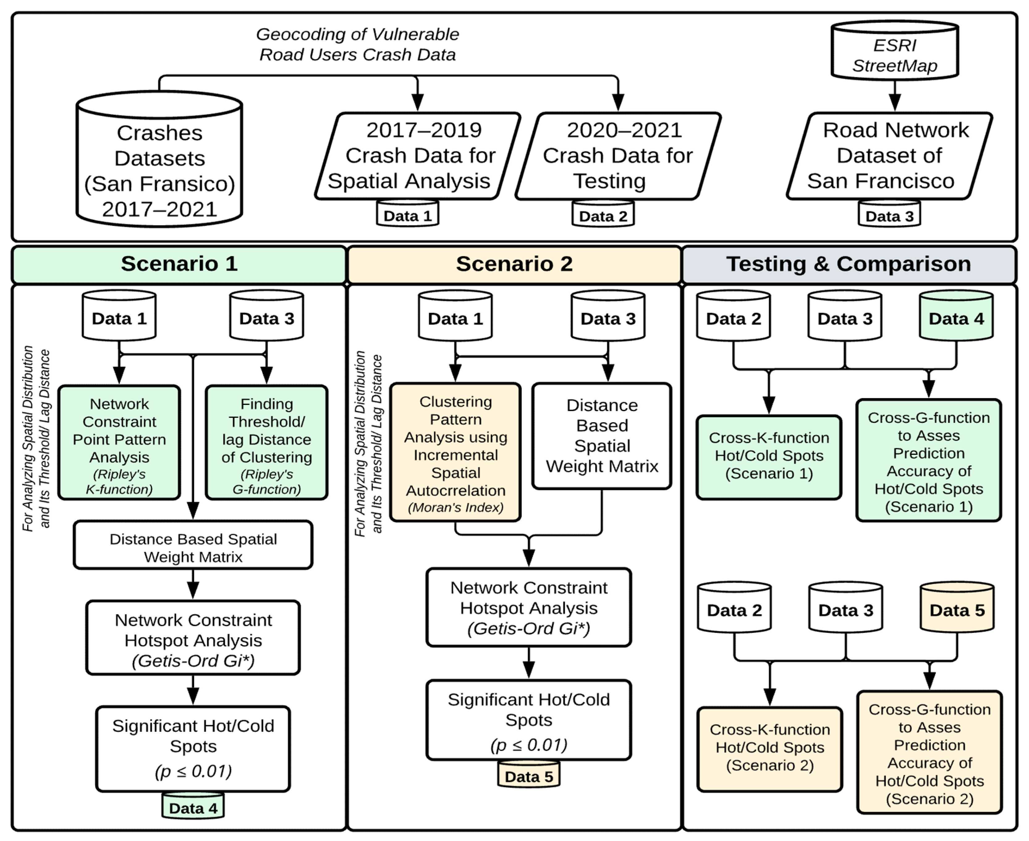
Multiple attributes, such as human error, traffic violations, and driving behavior, may be associated with crashes. Examples of the latter include speeding, inaccurate assumptions about other driver actions, failure to fasten seat belts, compromised sobriety, unsafe maneuvering, and tailgating [29,30,31,32]. Plotting crash locations on a map using a geographical information system (GIS) helps to visualize and identify hot spots that are high-risk locations. Analysts use different methods to identify hot spots, which are location clusters with statistical significance. Shahzad (2020) reviewed more than 80 articles and found that most analysts used Getis-Ord Gi* (30%), followed by kernel density estimation (KDE) (27%) and Moran’s Index analysis (22%) [3]. The approaches to identifying hot spots were based on a single method or a sequence of methods. Clustering methods for crashes have been employed since the early 1990s using individual crash points (latitude and longitude) as well as event-based approaches and link-based approaches [4]. For example, Erdogan et al. (2008) used KDE to identify high-density crash locations [33]. Gundogdu (2010) used Getis-Ord Gi* only to screen for hot spots [34]. Manepalli et al. (2011) used both Getis-Ord Gi* and KDE to map the hot spots that both methods identified [35]. Cáceres (2011) applied Getis-Ord Gi* and Moran’s I spatial autocorrelation to the same data to validate hot spot locations [36]. In another study [22], the Global Moran’s Index is used to identify the spatial pattern of data such as random, dispersed, or clustered data, and then the Getis-Ord Gi* or Local Moran’s Index is used [22]. The most common workflow was the use of Moran’s I to determine a threshold distance in the spatial autocorrelation and then apply Getis-Ord Gi* with that threshold distance, followed by KDE. The researchers used either planar space or linear networks in their spatial autocorrelation methods [14,15,37]. However, the studies found that network-based analysis produced more accurate results [3,11,19,26,38,39]. Another method to identify hot zones in multivariate modeling was through the use of the Mahalanobis distance [40,41]. By factoring in correlations between variables (e.g., location, time, weather, vehicle types), the Mahalanobis distance reveals hidden crash patterns that are missed by the traditional measures. An overview of the previous methodology used in the spatial analysis of crash data, including diagrams of the spatial analysis procedure used by researchers, is presented in Figure 2. In Figure 2, workflow 1 was used by [22,33,36], [22,36] then applied workflow 2 and workflow 3 after workflow 1; [15,22,26,34,38,42] employed workflow 3 and workflow 4; [18,19,21] employed workflow 5 and workflow 6 to find critical hot spots; workflow 7 was followed by [43,44] to identify hazardous locations for crashes.
Our literature review did not find any research that applied Moran’s I to identify clusters based on network-constrained analysis and then to find a threshold distance that would inform a subsequent network-constrained Getis-Ord Gi* hot spot analysis. This is important because using the Euclidean—or any other distance method other than the network-constrained distance—to find the threshold distance can lead to inaccurate results. Secondly, the use of the distance type should be the same across all the methods used in a sequence. For example, the only ready-to-use tool available in ArcGIS Map and ArcGIS Pro for finding the threshold distance is “Incremental Spatial Autocorrelation (ISA)”, which is based on the Global Moran’s I. ISA does not allow users to change the distance type used in the calculations other than Euclidean and Manhattan. However, in the case of Getis-Ord Gi*, users are given the option to switch between several distance types, including the actual network distances (calculated separately). To address this limitation, this research used Ripley’s K- and G-functions instead of ISA (Global Moran’s I), as shown in Figure 2, as the proposed workflow at number 8. Point pattern analysis and Moran’s Index are both statistical methods used to analyze spatial data, but they have some key differences. Point pattern analysis is used to identify patterns in the data—such as clusters or dispersion—at a local scale, while the Global Moran’s Index is used to measure the overall spatial autocorrelation for the entire dataset. Researchers have used this to find the threshold distance using the incremental spatial autocorrelation method. It is worth noting that the Local Moran’s Index helps to identify clustering at a local scale; however, estimating the threshold distance through the Local Moran’s Index involves a manual iterative process that could lead to precision errors. The K- and G-functions are used for point pattern analysis and are different from Moran’s Index because point pattern analysis methods are not sensitive to outliers, but may make assumptions about the underlying point process. On the other hand, Moran’s Index can be affected by outliers and makes assumptions, such as the normality and stationarity of the data. Additionally, Moran’s Index uses a quantitative value of the event to identify spatial autocorrelation among events. Figure 3 summarizes the distribution of the methods used based on the literature review.
The proportion of the frequency of the use of the methods in our reviewed literature are further summarized in Table 1, along with their general pros and cons.
The other methods category in Table 1 included econometric modeling, DBSCAN clustering, K-means clustering, Geographically Weighted Regression (GWR), machine learning approaches, and buffer analysis.

3. Methodology

The following subsections describe the study area, the data sources, and the methods developed to identify the crash clusters that involved vulnerable road users.

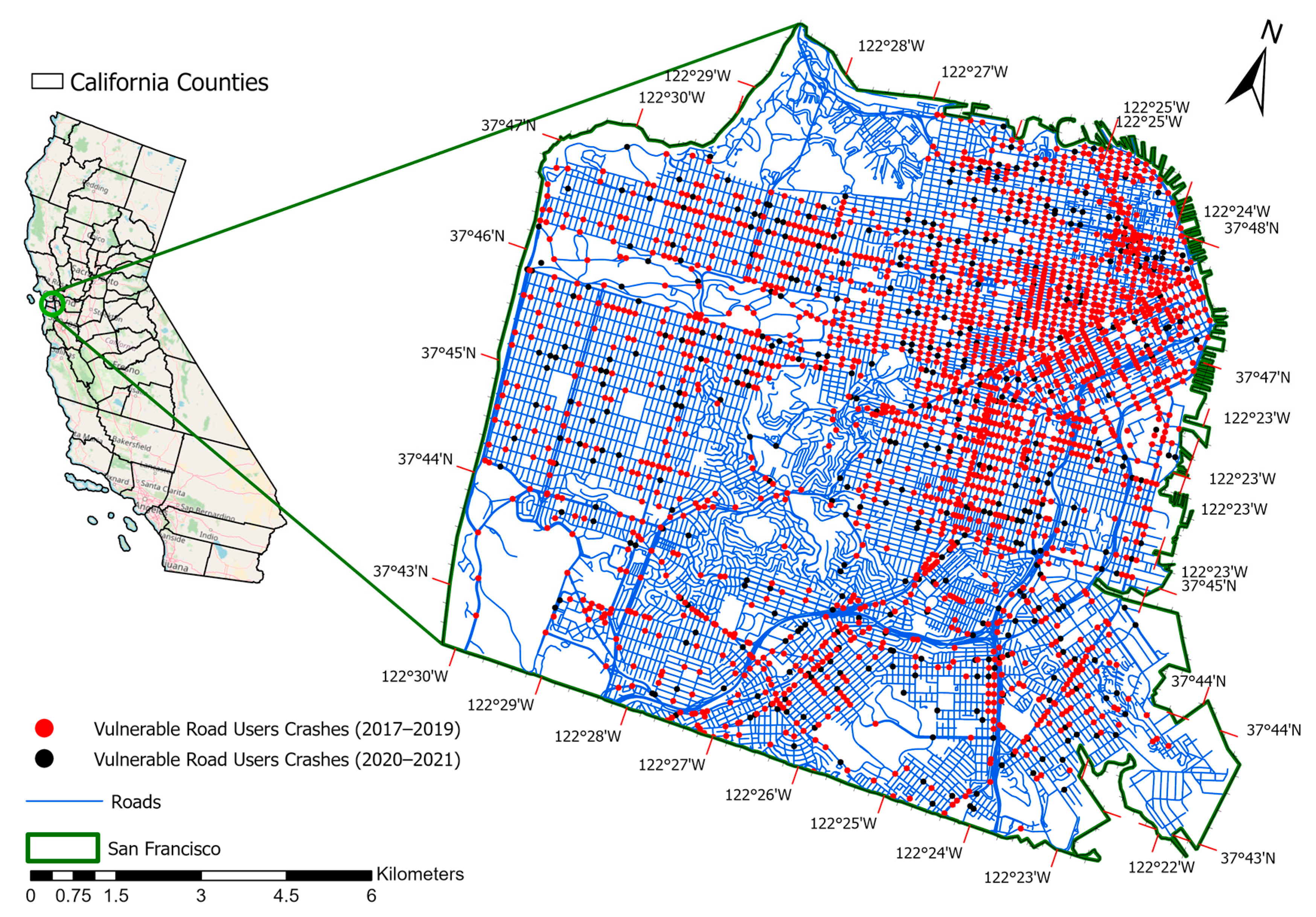
3.1. Study Area and Data

The study area was San Francisco, a California city and county that spans 46.9 square miles with a 2020 population of 0.875 million. The city of San Francisco was selected because of the availability of the crash data and its touristic importance in the U.S. According to the International Trade Administration (ITA) USA, San Francisco is among the top 10 cities in the U.S. visited by overseas tourists. In 2020, more than 400,000 foreigners visited San Francisco and the number of domestic tourists is even higher [52]. The implication is that there are many vulnerable road users in San Francisco, which provides a good case study. This case study uses two major data sets: crashes and the road network. TransBase Dashboard was the source of the crash dataset [53]. Among the 15,285 crashes that occurred between 2017–2021, a total of 5509 involved vulnerable road users (pedestrians and bicyclists). The hot spot analysis used 3816 (69.27%) data points from 1 January 2017 to 31 December 2019, (Table 2), and we used this data for training purposes. We used the remaining data set of 1693 (30.73%) crash points from 2020–2021 for testing the temporal robustness of the methods and evaluating the prediction accuracy of our suggested methodology based on the presence of clusters. Figure 4 depicts the study area and plots the crash locations as points.
The dataset contained only four severity levels of the KABCO scale [54]: fatal crashes (K), severe injury (A), other visible injury (B), and injuries with complaints of pain (C). ESRI’s ArcGIS StreetMap and speed profile data sources were used to estimate the travel time between the shortest travel distances among crash points on the road network. The ESRI speed variation data were based on hours of the day. Comparing a random subset of 20 distances and travel times from Google Maps with the results obtained from the network analyst using ESRI ArcGIS Pro 2.8 validated the accuracy of the topology and the hierarchy of the route selection. The road network was clipped to focus the analysis on the study area using the Clip tool in ArcGIS. The maps for both datasets used the WGS 1984 UTM Zone 15N-projected coordinate system with length and distance units in meters and speed units in kilometers per hour.

3.2. Methods

To achieve the goals of this research, we used a scenario-based methodology to evaluate alternative methods of finding threshold distances for crash hot spot analysis. In Scenario 1, we conducted clustering analysis using Ripley’s K-function with the actual road network distances as spatial weights for the testing data. Ripley’s K-function only identifies whether the crash data exhibit clustering. Subsequently, we use the G-function to find the maximum distance from each crash location to all other crash locations found in the respective cluster. This maximum distance became the threshold distance to be used in the hot spot analysis. Next, we conducted hot spot analysis using the Getis-Ord Gi* method to find hot and cold spots of crash locations.
In Scenario 2, we repeated the methodology that is commonly applied in the literature. First, we conducted ISA, which utilizes the Global Moran’s Index method with Euclidean distances for the conceptualization of spatial relationships among crashes. The outcome of the ISA established the threshold distance. Parallel to the ISA, we estimated the spatial weights using the actual road network distances. The “Generate Network Spatial Weights” tool of ArcGIS Pro provided the spatial weights. The spatial weights and threshold distance from the ISA were inputs for the subsequent Getis-Ord Gi* hot spot analysis, which provided hot and cold spots of crashes.
Finally, we compared the two scenarios using the cross-K-function and cross-G-function [14,55,56]. The testing data (2020–2021 data) are used as reference points and the outcome of scenario 1 and scenario 2 is used to find their accuracy. Among scenario 1 and scenario 2, the one that showed the most clusters was considered the more accurate scenario for finding hot spots and cold spots [14]. The subsequent sections of this paper discuss the details of the application of the cross-K-function and cross-G-function. Figure 5 presents a flow chart of the analytical workflow.
In summary, we employed two distinct methods during the initial phase: (1) network-constrained point pattern analysis (utilizing Ripley’s K-function and G-function) and (2) the Moran’s Index method followed by Getis-Ord Gi* to identify crash hot spots and cold spots. We then compared the results of these two approaches using a separate testing dataset that was not employed in the initial phase. To ascertain the temporal robustness of the identified hot and cold spots, we employed the cross-K-function and cross-G-function. Our accuracy determination is based on whether the crashes from the testing dataset cluster around the predicted hot and cold spots or vice versa.

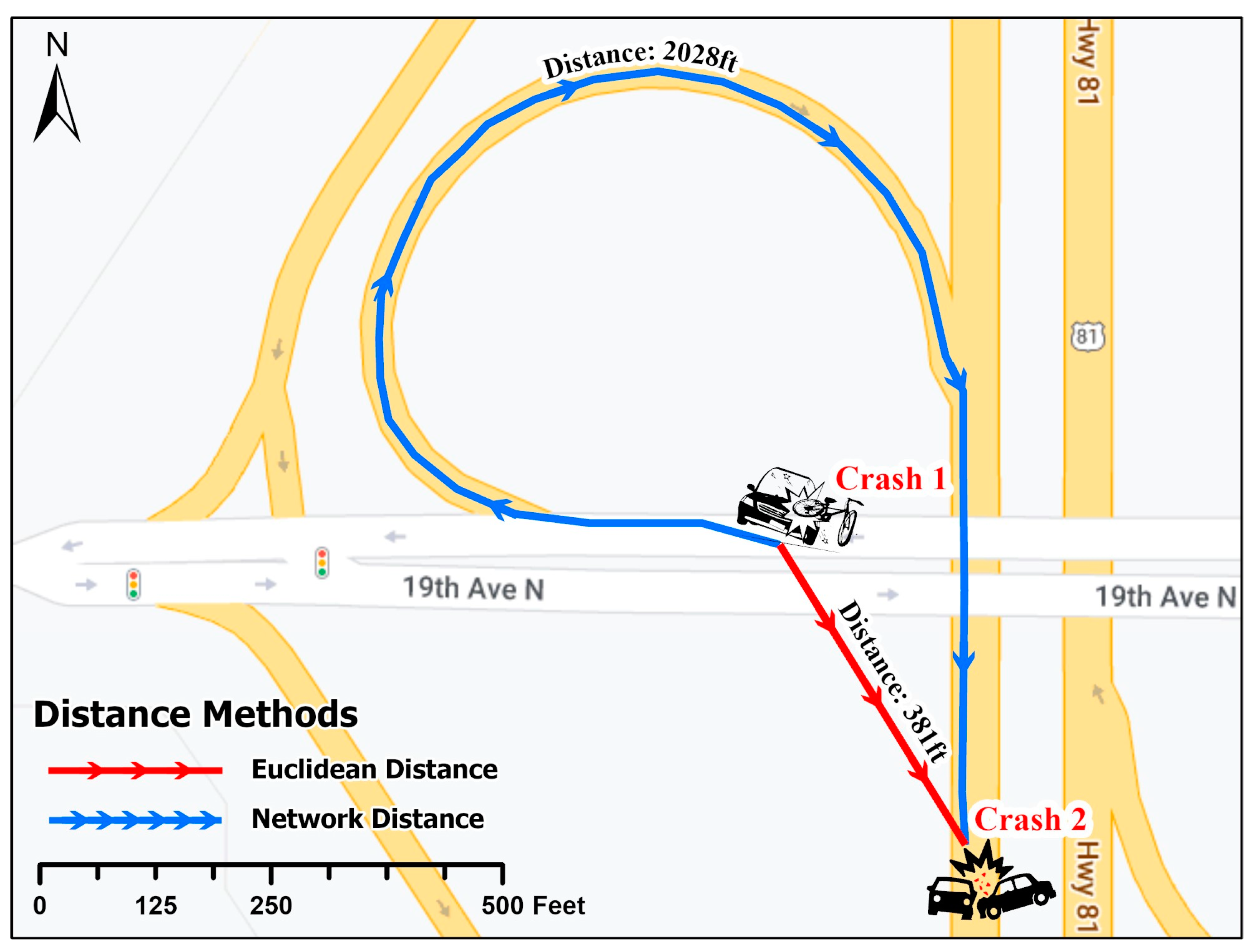
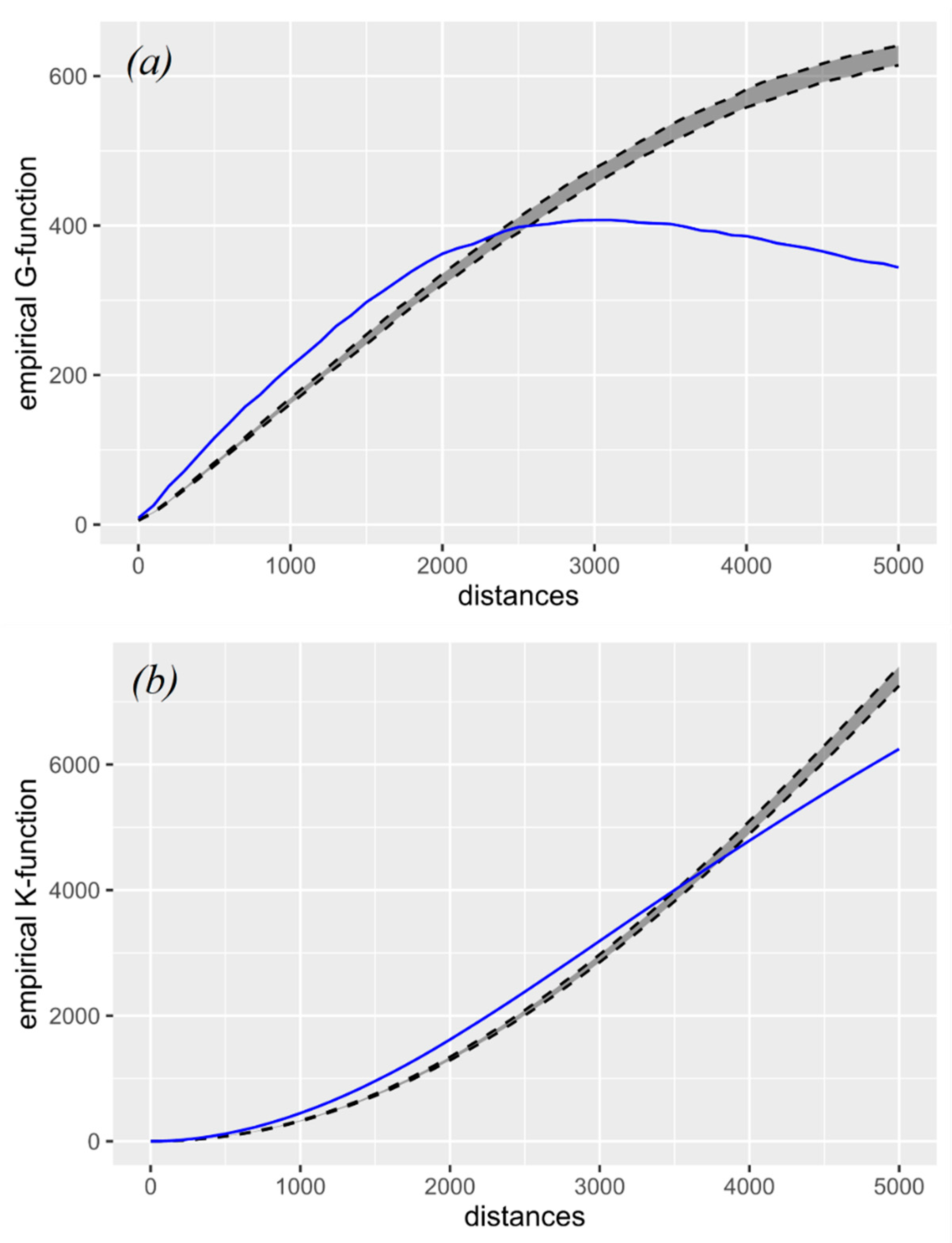
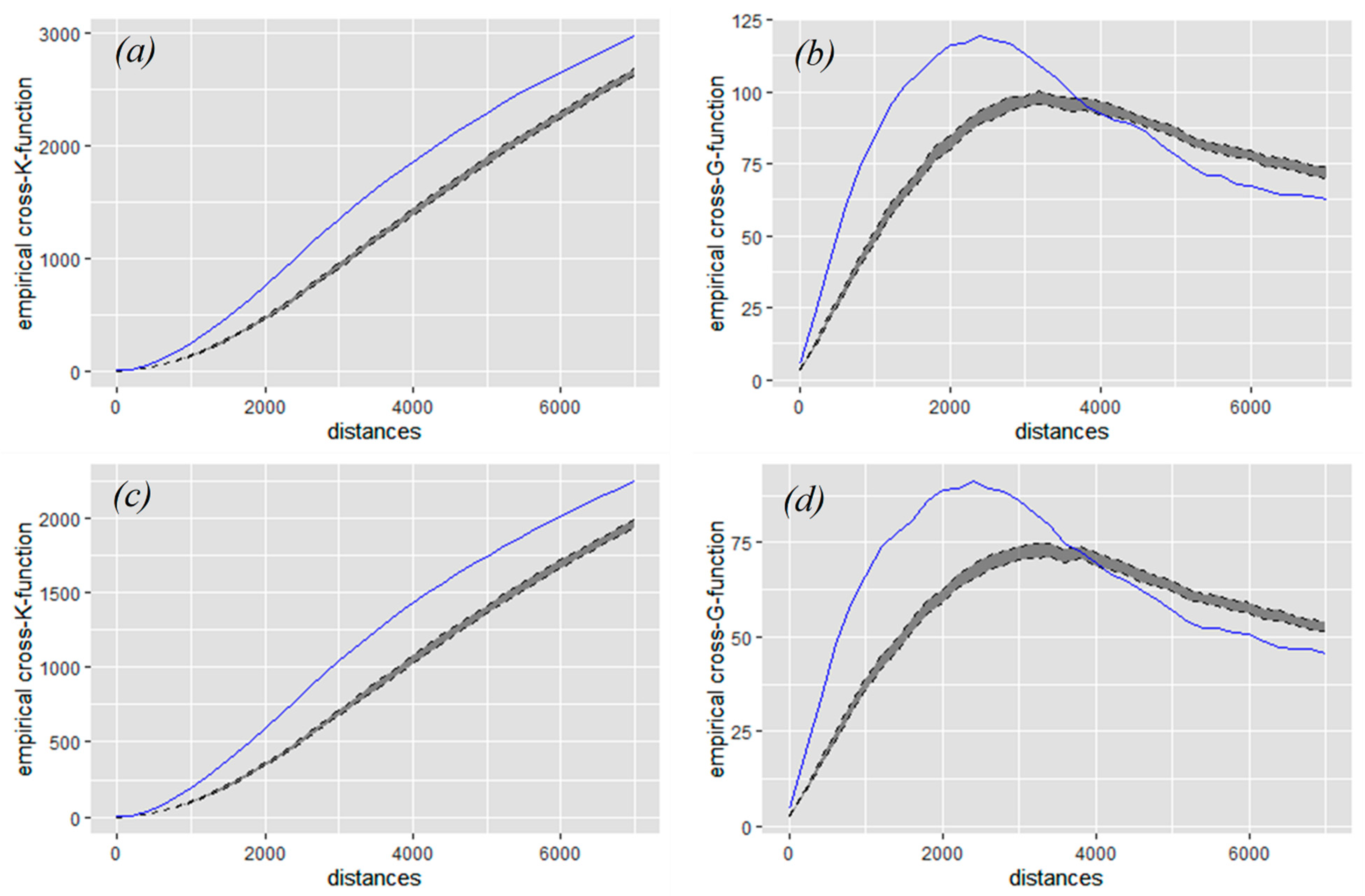
3.3. Network-Constrained Point Pattern Analysis: K-Function and G-Function

Ripley’s K-function is one of the most widely used methods of second-order point pattern analysis. The function summarizes the spatial dependence among data instances as a function of their separation distance. Ripley (1976) described the K-function for planer space [57]. Okabe and Sugihara (2012) later incorporated network constraints [14]. The K-function tests the spatial distribution of points relative to a random distribution at various spatial scales [15]. A Monte Carlo simulation can produce random reference data by creating random sample points on the network links. The K-function is:
K ^ r = 1 n ( n 1 ) i = 1 n j = 1 , j i n 1 D i j r
where K ^ r is the network value for all points where D i j r . D i j is the distance between point i to point j, and n is the number of points on a road network [55].
Most spatial autocorrelation tools require a threshold distance to detect clustering. Previous work in network-constrained local spatial autocorrelation identified the threshold distance manually by iterating the Moran’s I calculation across various distances [19]. The “Incremental Spatial Autocorrelation” tool of ArcGIS Pro calculates the Moran’s Index as a function of the distance up to a predefined maximum distance, and then selects the threshold distance for location autocorrelation analysis based on a peakz-statistic. Alternatively, the G-function, which is a modified version of the K-function, can directly compute a threshold distance [58]. The G-function is a pairwise correlation function that considers a subset of points that are within a narrow distance band. The G-function is as follows [55,56]:
G ^ r = 1 ( n 1 ) / L t i = 1 n j = 1 , j i n 1 D i j r
where L t is the total length of the network.
The workflow of this research used the cross-K-function to evaluate the accuracy of the cluster identification method. The cross-K-function helps to identify whether two points—points “ a ” and “b”—in two different datasets tend to be in proximity and follow a clustering pattern. The cross-K-function is:
C r o s s K ^ r = 1 ( n a n b ) i = 1 n a j = 1 n b 1 D i j r

3.4. Incremental Spatial Autocorrelation: Global Moran’s Index Analysis

Global Moran’s I is a statistical method that measures multi-dimensional and multi-directional spatial autocorrelation, which is a measure of the spatial dependency of the analyzed features [5,6]. Moran’s I statistics cover both the location of a feature and its attribute value simultaneously by defining its spatial co-variance of heterogeneity. The value of Moran’s I defines three pattern forms: dispersed, random, and clustered. The index value is as follows:
I = N i j W i j X i X ¯ ( X j X ¯ ) ( i j W i j ) W i j ( X i X ¯ ) ( X j X ¯ ) 2
where N is the number of instances, Xi is the variable value at a particular location, Xj is the variable value at another location, X ¯   is the mean value of the variable, and Wij is the distance weight between location i and location j.
The spatial statistics function from the ArcGIS Pro toolkit: Incremental Spatial Autocorrelation analyzes the spatial autocorrelation of crashes using Global Moran’s I. Global Moran’s I: the calculated Moran’s Index values are associated with a z-score that statistically explains the existence of clusters. The Moran’s Index ranges between +1 and −1. A value that approaches +1 suggests that there is clustering, a value near 0 suggests that the pattern is randomly dispersed, and a value that approaches −1 suggests that the pattern is dispersion or that there is spatial heterogeneity [21,22,59,60]. The null hypothesis of the statistical test on the z-score is that the data form a spatially random pattern. Hence, a p-value associated with thez-score that rejects the null hypothesis suggests that there is spatial clustering. The standardized z-score is:
Z = I E ( I ) V A R ( I )
E ( I ) = 1 ( N 1 )
V A R I = E I 2 E ( I ) 2
A z-score that is large enough to indicate a significant difference from randomness warrants further analysis to detect hot spots. The Incremental Spatial Autocorrelation identified a threshold distance for the subsequent hot spot analysis [35].

3.5. Advantages, Disadvantages, and Limitations

The advantages, disadvantages, and limitations of using points pattern analysis methods (K- and G-functions) and the Moran’s Index method are discussed in Table 3 and Table 4.

3.6. Network Constraint Local Indicator of Clusters: Getis-Ord Gi* Statistics

Getis-Ord Gi* (Gi*) identifies the location of incidence clusters based on statistical significance [8,9,35]. Gi* identifies the degree to which features within a certain distance (spatial lag) with high or low values surround a feature. The method calculates az-score that indicates the concentration ratio of a point feature surrounded by other point features with similar values, for example, features with high values surrounded by others with high values (high-high). Similarly, the method identifies points with low feature values surrounded by other points with low feature values (low-low). Highz-scores suggest the presence of a point cluster with high feature values. Similarly, lowz-scores suggest the presence of a point cluster with low feature values (cold spot). The calculation of Gi* is:
G i * d = j = 1 n W i j d x j X ¯ j = 1 n W i j ( d ) S [ n j = 1 n W i j 2 d ( j = 1 n W i j ( d ) ) 2 ] n 1
where G i * is thez-score, for instance, i within a distance d of instance j. The value x j   is the feature value, for j within distance d of instance i. W i j ( d ) is a binary spatial weight matrix as a function of the network travel distance d between instances i and j. The value n is the total number of instances under analysis. The weight matrix entry is 1 and 0 for instances that the method considers to be neighbors or not, respectively [42]. The method used the threshold distance obtained from the G-function to estimate the weight matrix. The value X ¯ is:
X ¯ = j = 1 n x j n
and the value S is:
S = j = 1 n x j n X ¯ 2
The analysis must then evaluate thez-score associated with the Gi* statistic within confidence intervals of 99%, 95%, and 90% [36,61]. One limitation we observed in the data was missing information in the elevation data. This is important because crashes that occur at locations such as underpasses and elevated structures, such as flyovers, can affect the network constraint distance, which may lead to some calculation errors.

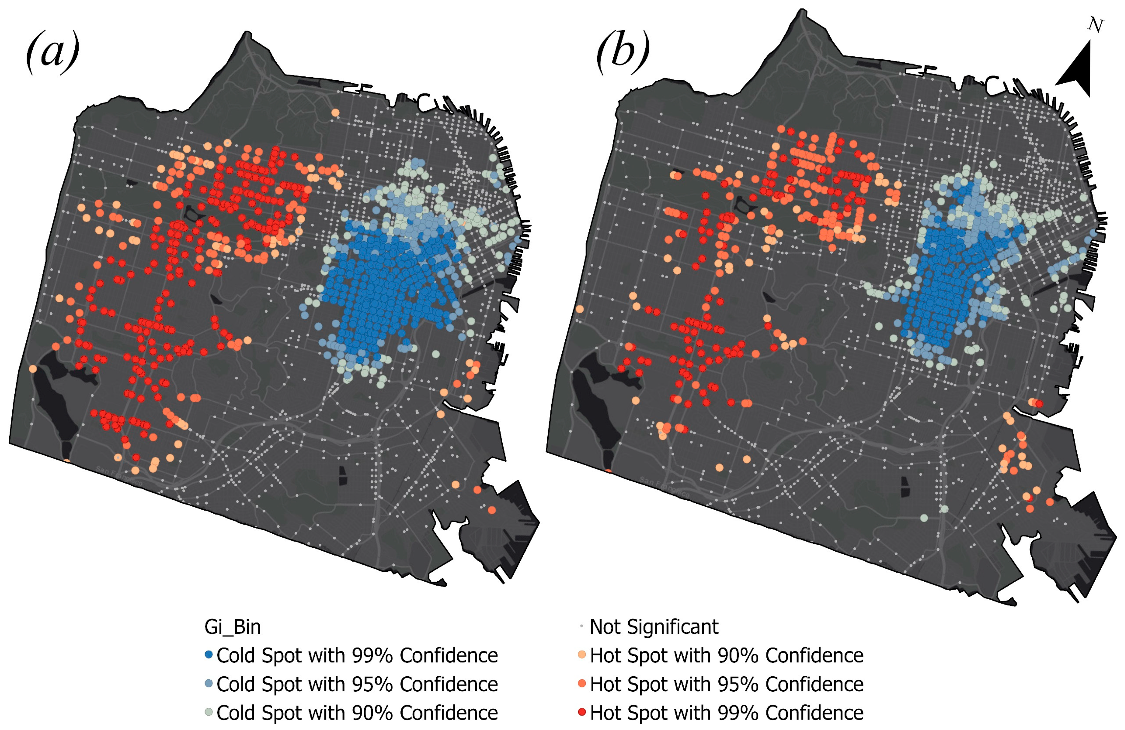
3.7. Definition of Hot Spots and Cold Spots

The definitions of hot and cold spots vary depending on the context and method used. For example, in one study, the method used to identify crash hot spots considered the number of serious injury crashes that took place within a defined segment length (500 m) over a span of 3 years, or if the number of fatalities was equal to or greater than 10 [62]. In our study, hot spots are locations where the Getis-Ord GI* statistics are positive with a significantz-score at a confidence level of 90% and above. Similarly, cold spots are locations where the Getis-Ord Gi* statistics are negative with a significantz-score at a confidence level of 90% and above. In other words, if there is a cluster of crashes where high injury severity crashes are surrounded by other high injury severity crashes, it is referred to as a hot spot. Conversely, if there is a cluster of low injury severity crashes surrounded by other low injury severity crashes, it is known as a cold spot.

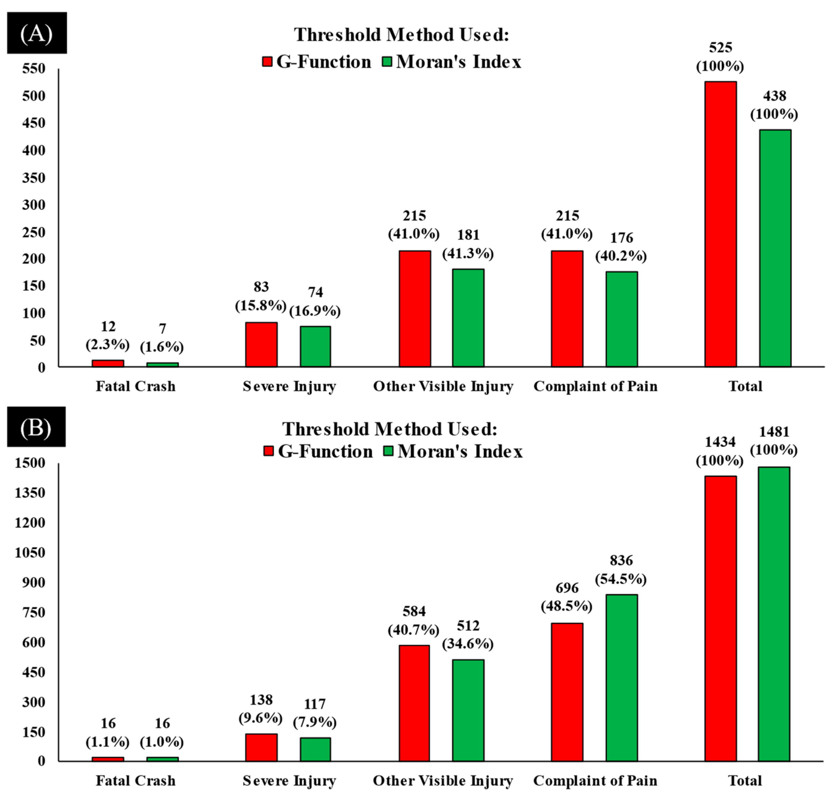
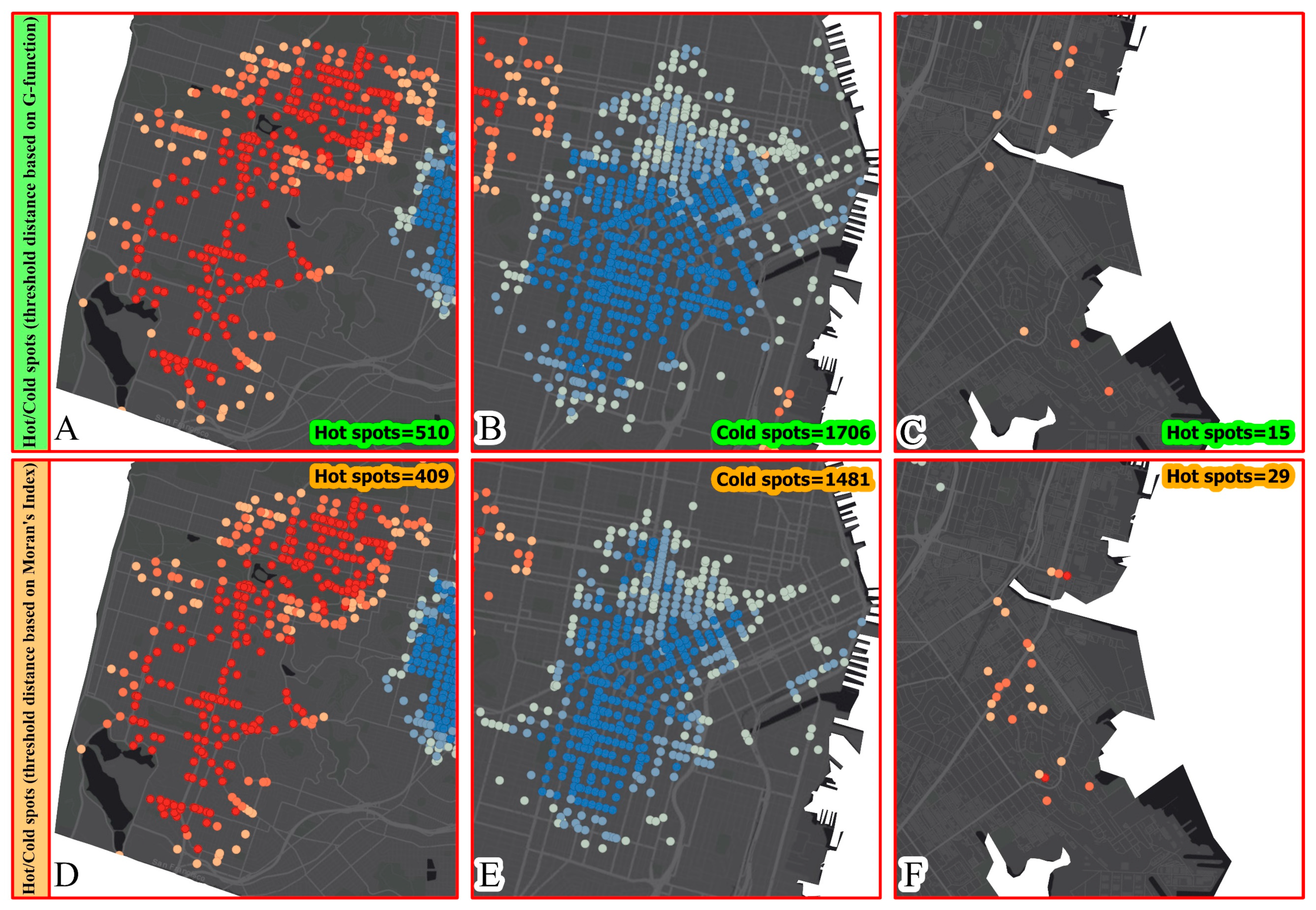
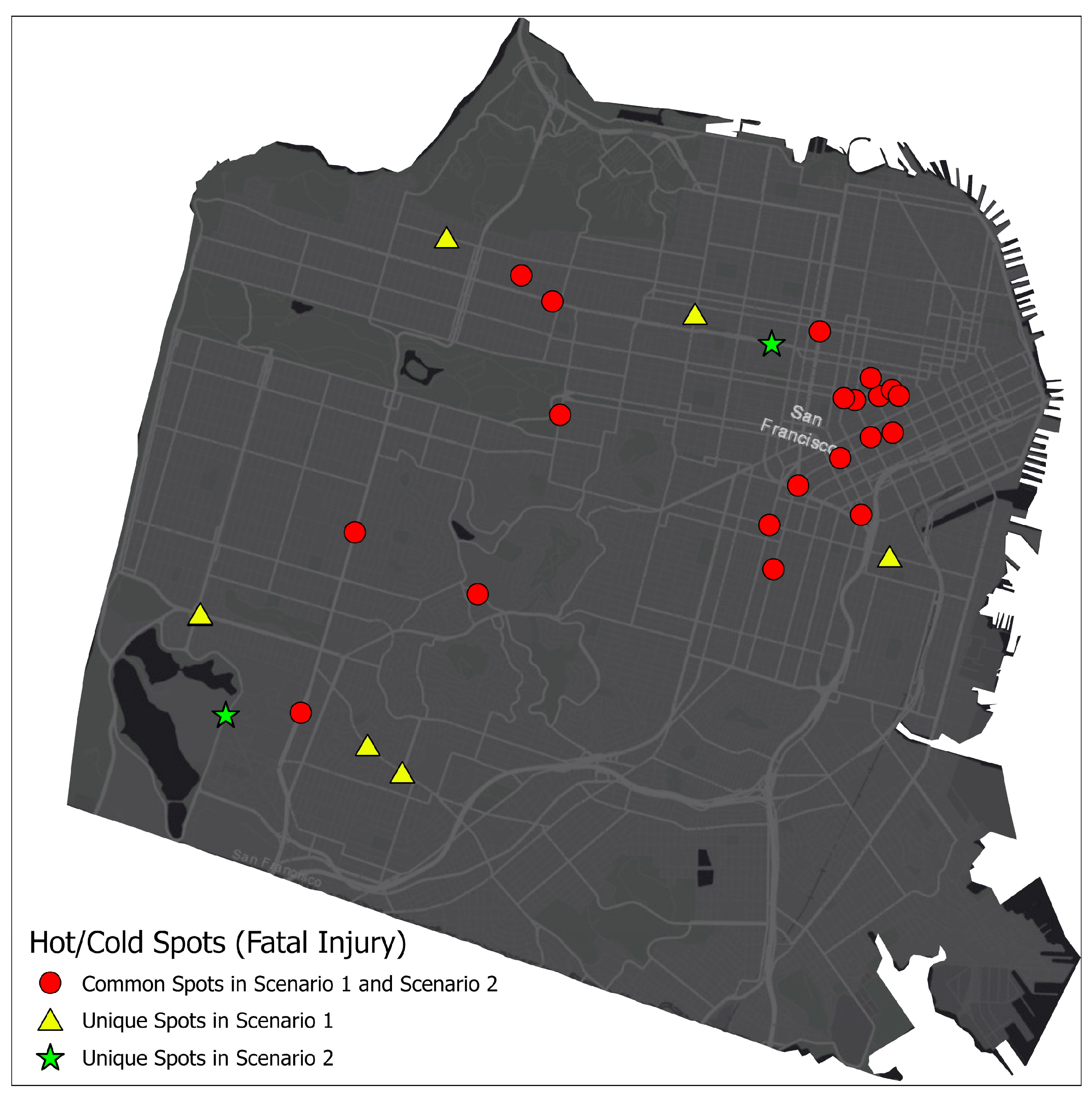
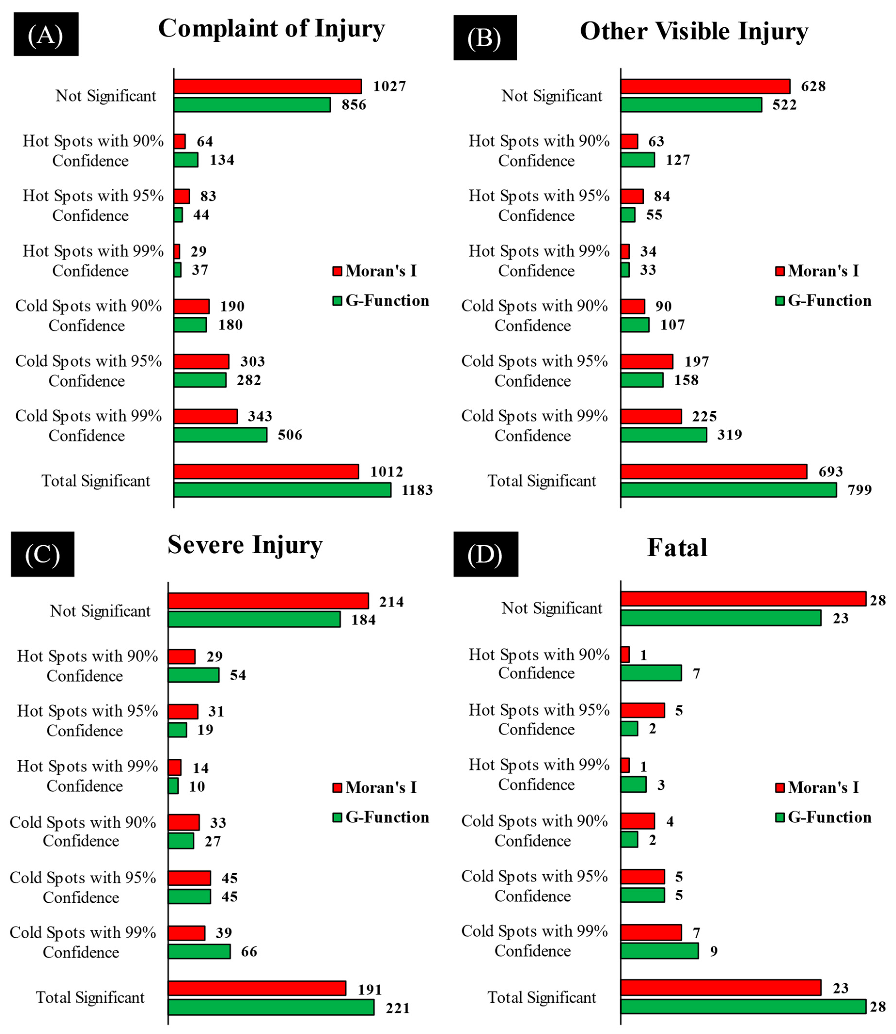
4. Results and Discussion

The point pattern analysis was carried out using the “SpNetwork” package developed by [55]. The package estimated the K-function and G-function values to identify the threshold distance, which the workflow later used to perform hot spot analysis. The hypothesis testing used 1000 Monte Carlo simulations, implemented with the R programming language, to create a random spatial distribution of crash locations on the road network. The distance increments for the function values were 50 m. The method considered the distribution of crashes to be clustered if the K ^ r value was greater than the confidence envelope of the random distribution. Values of K ^ r that were within the confidence envelope indicated a random distribution, while K ^ r values below the confidence envelope indicated a dispersion of crash events on the road network. Figure 6 presents the spatial distribution of the vulnerable road user crashes that occurred between 2017 and 2019. The ArcGIS Pro “Generate Network Spatial Weights” tool, available in the ESRI’s StreetMap road network, produced the spatial weights matrix. The cut-off distance parameter of the tool was set to the threshold distance obtained from the G-function.
In Figure 6, the solid line is based on the G- and K-function values of the crash locations. The envelope bounded by upper and lower dashed lines indicates the expected K-value for spatial randomness at a significance level of 0.05. The x-axis shows the distance in meters. The G-function indicated that the threshold distance for clustering was 2300 m (Figure 6a). The K-function indicated that, within a 95% confidence interval, there is a significant clustering of vulnerable road user crashes up to 3600 m (Figure 6b). The threshold distance obtained from the Global Moran’s I calculation used a weights matrix based on the Euclidean distances. The “incremental spatial autocorrelation” tool in ArcGIS Pro calculated the Global Moran’s I with the Euclidean distances to produce the threshold distance [63]. The starting distance was set to 50 m and the increment was 50 m. The results showed two peaks of the Moran’s Index z-score: the first peak was at 150 m (z-score = 3.143, Moran’s I = 0.039), and the next peak, before losing the strength of spatial autocorrelation, was at 1400 m (z-score = 5.699, Moran’s I = 0.009). The analysis selected the threshold distance at the second peak at 1400 m because the clustering was more pronounced there.
The threshold distances obtained from both the G- and K-functions were greater than those obtained from the Global Moran’s I calculation because the latter used the Euclidean distance between points.
Figure 7a shows the results of the Getis-Ord Gi* hot spot analysis using network-constrained travel distances. Figure 7b shows the results based on Moran’s I Euclidean threshold distance of 1400 m. The Gi* method based on network threshold distances included 16.3% more locations in the combined hot and cold spots (Figure 8). Speed and congestion differences in the downtown area relative to the rest of the city may have influenced the separation of the hot and cold spots. This satisfies the intuition that vulnerable road users are more at risk where speed limits are higher, or equivalently, where traffic is less congested [64,65,66].
The injury severity proportions for the hot spot locations based on the Gi* method using network distance thresholds were 2.3% (12), 15.8% (83), 41% (215), and 41% (215) for fatal, severe, visible, and pain injuries, respectively. Comparatively, the proportions using the Euclidean distance threshold were 1.6% (7), 17.3% (74), 41.1% (176), and 42.3% (181) for fatal, severe, visible, and pain injuries, respectively. As shown in Figure 8, the proportion of crash injury severity was 1.1% (16), 9.6% (138), 40.7% (548), and 48.5% (48.5%) for fatal, severe, visible, and pain injuries (when G-Function is used for finding threshold distance). Similarly, for the Gi*-based cold spot locations, the proportions of injury severity of crashes identified as cold spots using the Euclidean distance were 1.0% (16), 7.9% (117), 34.6% (512), and 54.5% (836) for fatal, severe, visible, and pain injuries.
Figure 9C,F shows the hot spots around the I-280 (freeway). As explained in Figure 1, Moran’s Index uses the Euclidean distance and therefore identified more hot spots because it ignored the network topology. However, the G-function incorporated the network topology and, therefore, identified fewer hot spots (15 vs. 29) with Getis-Ord Gi*, as shown in Figure 9C. Figure 10 shows the difference between the results of the two scenarios by highlighting the common hot/cold spots and unique spots identified by each of the scenarios. There are unique locations that were identified in Scenario 1 but were not identified in Scenario 2. These unique locations are presented in yellow triangles. Similarly, the green stars are the unique locations that were identified in Scenario 2 but were not identified in Scenario 1.
Figure 11 presents a more detailed comparison of the hot and cold spots at 90%, 95%, and 99% confidence levels based on the results of the Gi* hot spot analysis. The number of insignificant crash locations for each crash severity category is based less on the network threshold distances derived from the G-function than for those derived using Moran’s I method with Euclidean distance thresholds. Conversely, for each crash severity category at the 0.1 significance level (90% confidence level) of clustering, the number of hot spots with the G-function-derived network distance threshold was greater.
The workflow presented in Figure 5 shows that the cross-K-function and cross-G-function tested the accuracy of Scenario 1 and Scenario 2. The workflow used vulnerable road user crash data for the years 2020 and 2021 (testing data) to check whether the crash locations tended to cluster around the predicted hot spots to show a spatial correlation between datasets [50]. Figure 12 shows the results of the cross-K-function and the cross-G-function. The empirical cross-K-function and cross-G-function values in Figure 12a,b for Scenario 1 are higher than those of Figure 12c,d for Scenario 2. The observed G-function value in Figure 12b remained above the upper envelope curve at a 0.05 significance level until 3600 m, with more crash points above the grey area of randomness.
In Figure 12d, the observed G-function remained above the 0.05 significance level up to 3400 m, with fewer crash points showing a cluster pattern. The interpretation of this result is that the predicted crashes clustered around the same hot spots. The Y-axis of the cross-K-function shows the cumulative number of crash points, whereas that of the cross-G-function does not. The main conclusion from these results is that the vulnerable road user crashes that occurred in 2020–2021 tended to be more clustered in the hot spots and cold spots, as shown in Figure 9A–C.

5. Summary and Conclusions

This study presents a novel approach for determining the threshold distance required to compute local spatial autocorrelation to identify clusters of statistical significance. Historically, the Euclidean distance has been the predominant method employed to establish a global clustering distance threshold, even in instances where network-constrained local spatial autocorrelation models were utilized. However, this approach may not always be the best fit for identifying clusters of statistical significance, particularly when studying urban areas where the density of the population and road infrastructure is high.
The method proposed in this study utilizes the K-function and G-function to detect global clustering patterns in the study areas by identifying the distance at which the point data exhibit clustering. These methods take into account the underlying network structure of the study area, which is critical for understanding the spatial patterns of crashes involving vulnerable road users. One of the key benefits of using the K-function and G-function is that they can be applied to a wide range of data at a large scale, including point data and areal data; however, Moran’s Index is scale-dependent. This versatility makes them a valuable tool for practitioners in different fields, such as transportation planning, traffic safety, and public health. Additionally, the R package “SpNetwork” offers a greater number of distance windows and a larger distance range, resulting in increased resolution for selecting an appropriate distance threshold. Conversely, the “Incremental Spatial Autocorrelation” tool in ArcMap and ArcGIS Pro, which utilizes the Global Moran’s Index, has a limited number of incremental distance windows (maximum 30). A case study of San Francisco was conducted and revealed that crashes involving vulnerable road users were highly concentrated in the downtown area (central business district). One limitation of this study is that it only focused on one city, San Francisco. Further, we used the crash data of 2020–2021 as testing data, which may have different traffic volume trends because of the COVID-19 outbreak and other Non-Pharmaceutical Interventions (NPI), which may have affected the traffic [67]. Therefore, future work should include more case studies in different urban areas to validate the proposed methods and to understand the generalizability of the findings, and use data from a period when COVID-related NPIs were not in place. Utilizing a larger distance window can negatively impact the autocorrelation results and using Euclidean distances for the weight matrix calculation rather than the actual network distances may lead to false indications of strong clustering at shorter distances, particularly when using the Global Moran’s Index. However, if spatial weights based on the actual distance and travel time are used as inputs for the Global Moran’s Index, better results may be obtained. The proposed method of utilizing the K- and G-functions in this study yielded more clusters than the methods that employ Moran’s I, providing decision-makers with optimal hot/cold spot locations for crash mitigation. Priority should be given to hot/cold spots of fatal and severe injury locations, as shown in Figure 10, as an example of hot/cold spots of fatal crashes as dealing with more hot/cold spots can be one of the challenges.
The study also employed the cross-K- and cross-G-functions to determine the precision of the outcome from two scenarios using the threshold distances established by the K-/G-functions as well as from the Moran’s Index. The reference dataset served as the test data. The analysis of the cross-K- and cross-G-functions showed that when the threshold distances were determined using the network-constrained K- and G-functions, there was a greater degree of coherence with the testing data in the spatial patterns compared to when Euclidean distance-based threshold distances were used in the Moran’s Index analysis. This method represents a new way of evaluating the accuracy of the outcomes obtained through different competing methods. The results of this study can be applied by practitioners in the transportation and urban planning field to improve road safety in urban areas by identifying specific hot spots where interventions are needed.

Author Contributions

Conceptualization, M.F.H., D.M. and R.B.; Methodology, M.F.H., D.M. and R.B.; Software, M.F.H.; Validation, M.F.H., D.M. and R.B.; Formal Analysis, M.F.H.; Investigation, M.F.H.; Data Curation, M.F.H.; Writing—Original Draft Preparation, M.F.H.; Writing—Review and Editing, M.F.H., D.M., R.B. and B.R.; Visualization, M.F.H.; Supervision, D.M. and R.B. All authors have read and agreed to the published version of the manuscript.

Funding

This research received no specific grant or funding from any funding agency or source.

Institutional Review Board Statement

Not applicable.

Informed Consent Statement

Not applicable.

Data Availability Statement

Data source is as cited in the paper.

Conflicts of Interest

The authors declare no conflict of interest.

References

  1. NHTSA. Vulnerable Road Users (VRUs)—Publication Topic—CrashStats—NHTSA—DOT. Available online: https://crashstats.nhtsa.dot.gov/#!/PublicationList/127 (accessed on 30 July 2022).
  2. Ziakopoulos, A.; Yannis, G. A review of spatial approaches in road safety. Accid. Anal. Prev. 2020, 135, 105323. [Google Scholar] [CrossRef]
  3. Shahzad, M. Review of road accident analysis using GIS technique. Int. J. Inj. Control. Saf. Promot. 2020, 27, 472–481. [Google Scholar] [CrossRef]
  4. Yao, S.; Loo, B.P.Y.; Yang, B.Z. Traffic collisions in space: Four decades of advancement in applied GIS. Ann. Gis 2016, 22, 1–14. [Google Scholar] [CrossRef]
  5. Moran, P.A. Notes on continuous stochastic phenomena. Biometrika 1950, 37, 17–23. [Google Scholar] [CrossRef]
  6. Moran, P.A.P. The Interpretation of Statistical Maps. J. R. Stat. Soc. Ser. B 1948, 10, 243–251. Available online: https://www.jstor.org/stable/2983777 (accessed on 10 August 2023). [CrossRef]
  7. Ripley, B.D. Modeling Spatial Patterns. J. Roy. Stat. Soc. B Met. 1977, 39, 172–212. Available online: https://www.jstor.org/stable/2984796 (accessed on 10 August 2023). (In English).
  8. Getis, A.; Ord, J.K. The Analysis of Spatial Association by Use of Distance Statistics. Geogr. Anal. 1992, 24, 189–206. [Google Scholar] [CrossRef]
  9. Ord, J.K.; Getis, A. Local Spatial Autocorrelation Statistics: Distributional Issues and an Application. Geogr. Anal. 1995, 27, 286–306. [Google Scholar] [CrossRef]
  10. Anselin, L. Local Indicators of Spatial Association—LISA. Geogr. Anal. 1995, 27, 93–115. [Google Scholar] [CrossRef]
  11. Ulak, M.B.; Ozguven, E.E.; Vanli, O.A.; Horner, M.W. Exploring alternative spatial weights to detect crash hotspots. Comput. Environ. Urban Syst. 2019, 78, 101398. [Google Scholar] [CrossRef]
  12. ESRI. Best Practices for Selecting a Fixed Distance Band Value ArcGIS Pro|Documentation. Available online: https://pro.arcgis.com/en/pro-app/latest/tool-reference/spatial-statistics/choosingdistanceband.htm (accessed on 20 May 2023).
  13. Tobler, W.R. A Computer Movie Simulating Urban Growth in the Detroit Region. Econ. Geogr. 1970, 46, 234. [Google Scholar] [CrossRef]
  14. Okabe, A.; Sugihara, K. Spatial Analysis along Networks: Statistical and Computational Methods; John Wiley and Sons Ltd.: Hoboken, NJ, USA, 2012; pp. 1–288. [Google Scholar] [CrossRef]
  15. Yamada, I.; Thill, J.C. Comparison of planar and network K-functions in traffic accident analysis. J. Transp. Geogr. 2004, 12, 149–158. [Google Scholar] [CrossRef]
  16. Alam, M.S.; Tabassum, N.J. Spatial pattern identification and crash severity analysis of road traffic crash hot spots in Ohio. Heliyon 2023, 9, e16303. [Google Scholar] [CrossRef]
  17. Islam, M.K.; Reza, I.; Gazder, U.; Akter, R.; Arifuzzaman, M.; Rahman, M.M. Predicting Road Crash Severity Using Classifier Models and Crash Hotspots. Appl. Sci. 2022, 12, 11354. [Google Scholar] [CrossRef]
  18. Khan, I.U.; Vachal, K.; Ebrahimi, S.; Wadhwa, S.S. Hotspot analysis of single-vehicle lane departure crashes in North Dakota. IATSS Res. 2023, 47, 25–34. [Google Scholar] [CrossRef]
  19. Lee, M.; Khattak, A.J. Case Study of Crash Severity Spatial Pattern Identification in Hot Spot Analysis. Transp. Res. Rec. 2019, 2673, 684–695. [Google Scholar] [CrossRef]
  20. Ouni, F.; Belloumi, M. Pattern of road traffic crash hot zones versus probable hot zones in Tunisia: A geospatial analysis. Accid. Anal. Prev. 2019, 128, 185–196. [Google Scholar] [CrossRef]
  21. Prasannakumar, V.; Vijith, H.; Charutha, R.; Geetha, N. Spatio-temporal clustering of road accidents: GIS based analysis and assessment. Procedia—Soc. Behav. Sci. 2011, 21, 317–325. [Google Scholar] [CrossRef]
  22. Soleimani, M.; Bagheri, N. Spatio-temporal analysis of head injuries in northwest Iran. Spat. Inf. Res. 2022, 1, 1–16. [Google Scholar] [CrossRef]
  23. Thakali, L.; Kwon, T.J.; Fu, L. Identification of crash hotspots using kernel density estimation and kriging methods: A comparison. J. Mod. Transp. 2015, 23, 93–106. [Google Scholar] [CrossRef]
  24. Truong, L.T.; Somenahalli, S.V.C. Using GIS to identify pedestrian- vehicle crash hot spots and unsafe bus stops. J. Public Transp. 2011, 14, 99–114. [Google Scholar] [CrossRef]
  25. Ziakopoulos, A. Spatial analysis of harsh driving behavior events in urban networks using high-resolution smartphone and geometric data. Accid. Anal. Prev. 2021, 157, 106189. [Google Scholar] [CrossRef]
  26. Khalid, S.; Shoaib, F.; Qian, T.; Rui, Y.; Bari, A.I.; Sajjad, M.; Shakeel, M.; Wang, J. Network Constrained Spatio-Temporal Hotspot Mapping of Crimes in Faisalabad. Appl. Spat. Anal. Policy 2018, 11, 599–622. [Google Scholar] [CrossRef]
  27. Özcan, M.; Küçükönder, M. Investigation of Spatiotemporal Changes in the Incidence of Traffic Accidents in Kahramanmaraş, Turkey, Using GIS-Based Density Analysis. J. Indian Soc. Remote Sens. 2020, 48, 1045–1056. [Google Scholar] [CrossRef]
  28. Wang, S.H.; Chen, Y.Y.; Huang, J.L.; Liu, Z.; Li, J.; Ma, J.M. Spatial relationships between alcohol outlet densities and drunk driving crashes: An empirical study of Tianjin in China. J. Saf. Res. 2020, 74. [Google Scholar] [CrossRef]
  29. Huertas-Leyva, P.; Baldanzini, N.; Savino, G.; Pierini, M. Human error in motorcycle crashes: A methodology based on in-depth data to identify the skills needed and support training interventions for safe riding. Traffic Inj. Prev. 2021, 22, 294–300. [Google Scholar] [CrossRef]
  30. Pawar, D.S.; Patil, G.R. Response of major road drivers to aggressive maneuvering of the minor road drivers at unsignalized intersections: A driving simulator study. Transp. Res. Part F Traffic Psychol. Behav. 2018, 52, 164–175. [Google Scholar] [CrossRef]
  31. Rowe, R.; Roman, G.D.; McKenna, F.P.; Barker, E.; Poulter, D. Measuring errors and violations on the road: A bifactor modeling approach to the Driver Behavior Questionnaire. Accid. Anal. Prev. 2015, 74, 118–125. [Google Scholar] [CrossRef]
  32. Yue, L.; Abdel-Aty, M.; Wu, Y.; Zheng, O.; Yuan, J. In-depth approach for identifying crash causation patterns and its implications for pedestrian crash prevention. J. Saf. Res. 2020, 73, 119–132. [Google Scholar] [CrossRef]
  33. Erdogan, S.; Yilmaz, I.; Baybura, T.; Gullu, M. Geographical information systems aided traffic accident analysis system case study: City of Afyonkarahisar. Accid. Anal. Prev. 2008, 40, 174–181. [Google Scholar] [CrossRef]
  34. Gundogdu, I.B. Applying linear analysis methods to GIS-supported procedures for preventing traffic accidents: Case study of Konya. Saf. Sci. 2010, 48, 763–769. [Google Scholar] [CrossRef]
  35. Manepalli, U.R.R.; Bham, G.H.; Kandada, S. Evaluation of Hot-Spots Identification Using Kernel Density Estimation and Getis-ord on I-630. In Proceedings of the 3rd International Conference on Road Safety and Simulation, Indianapolis Indiana, IN, USA, 14–16 September 2011; Available online: http://pubs.trb.org/onlinepubs/conferences/2011/RSS/2/Manepalli,UR.pdf (accessed on 20 May 2023).
  36. Cáceres, C.F. Using GIS in Hotspots Analysis and for Forest Fire Fisk Zones Mapping in the Yeguare Region, Southeastern Honduras. Pap. Resour. Anal. 2011, 13, 1–14. Available online: http://gis.smumn.edu/GradProjects/CaceresC.pdf (accessed on 20 May 2023).
  37. Okabe, A.; Okunuki, K.I. A Computational Method for Estimating the Demand of Retail Stores on a Street Network and its Implementation in GIS. Trans. GIS 2001, 5, 209–220. [Google Scholar] [CrossRef]
  38. Shafabakhsh, G.A.; Famili, A.; Bahadori, M.S. GIS-based spatial analysis of urban traffic accidents: Case study in Mashhad, Iran. J. Traffic Transp. Eng. 2017, 4, 290–299. [Google Scholar] [CrossRef]
  39. Ulak, M.B.; Ozguven, E.E.; Spainhour, L.; Vanli, O.A. Spatial investigation of aging-involved crashes: A GIS-based case study in Northwest Florida. J. Transp. Geogr. 2017, 58, 71–91. [Google Scholar] [CrossRef]
  40. Osama, A.; Sayed, T. A Novel Approach for Identifying, Diagnosing, and Treating Active Transportation Safety Issues. Transp. Res. Rec. 2019, 2673, 813–823. [Google Scholar] [CrossRef]
  41. Osama, A.; Sayed, T.; Sacchi, E. A Novel Technique to Identify Hot Zones for Active Commuters’ Crashes. Transp. Res. Rec. 2018, 2672, 266–276. [Google Scholar] [CrossRef]
  42. Peeters, A.; Zude, M.; Käthner, J.; Ünlü, M.; Kanber, R.; Hetzroni, A.; Gebbers, R.; Ben-Gal, A. Getis-Ord’s hot- and cold-spot statistics as a basis for multivariate spatial clustering of orchard tree data. Comput. Electron. Agric. 2015, 111, 140–150. [Google Scholar] [CrossRef]
  43. Park, S.H.; Jang, K.; Kim, D.K.; Kho, S.Y.; Kang, S. Spatial analysis methods for identifying hazardous locations on expressways in Korea. Sci. Iran. 2015, 22, 1594–1603. [Google Scholar]
  44. Pirdavani, A.; Bellemans, T.; Brijs, T.; Wets, G. Application of Geographically Weighted Regression Technique in Spatial Analysis of Fatal and Injury Crashes. J. Transp. Eng. 2014, 140, 04014032. [Google Scholar] [CrossRef]
  45. Acharya, T.D.; Yoo, K.W.; Lee, D.H. GIS-based spatio-Temporal analysis of marine accidents database in the coastal zone of Korea. J. Coast. Res. 2017, 33, 114–118. [Google Scholar] [CrossRef]
  46. Hegyi, P.; Borsos, A.; Koren, C. Searching possible accident black spot locations with accident analysis and gis software based on GPS coordinates. Pollack Period. 2017, 12, 129–140. [Google Scholar] [CrossRef]
  47. Yu, H.; Liu, P.; Chen, J.; Wang, H. Comparative analysis of the spatial analysis methods for hotspot identification. Accid. Anal. Prev. 2014, 66, 80–88. [Google Scholar] [CrossRef]
  48. Zahran, E.-S.M.M.; Tan, S.J.; Amirah, N.; Binti, A.; Asri Putra, M.; Hie, E.; Tan, A.; Yap, Y.H.; Kartina, E.; Rahman, A. Evaluation of various GIS-based methods for the analysis of road traffic accident hotspot. MATEC Web Conf. 2019, 258, 03008. [Google Scholar] [CrossRef]
  49. ESRI. Spatial Autocorrelation (Global Moran’s I) (Spatial Statistics)—ArcGIS Pro|Documentation. Available online: https://pro.arcgis.com/en/pro-app/latest/tool-reference/spatial-statistics/spatial-autocorrelation.htm (accessed on 20 May 2023).
  50. Ulak, M.B.; Kocatepe, A.; Yazici, A.; Ozguven, E.E.; Kumar, A. A stop safety index to address pedestrian safety around bus stops. Saf. Sci. 2021, 133, 105017. [Google Scholar] [CrossRef]
  51. Kazmi, S.S.A.; Ahmed, M.; Mumtaz, R.; Anwar, Z. Spatiotemporal Clustering and Analysis of Road Accident Hotspots by Exploiting GIS Technology and Kernel Density Estimation. Comput. J. 2020, 65, 155–176. [Google Scholar] [CrossRef]
  52. ITA. US States & Cities Visited by Overseas Travelers. 2023. Available online: https://www.trade.gov/data-visualization/us-states-cities-visited-overseas-travelers (accessed on 10 August 2023).
  53. SFgov. TransBASE Dashboard. Available online: https://transbase.sfgov.org/dashboard/dashboard.php (accessed on 6 March 2022).
  54. FHWA. KABCO Injury Classification Scale and Definition. Available online: https://safety.fhwa.dot.gov/hsip/spm/conversion_tbl/pdfs/kabco_ctable_by_state.pdf (accessed on 6 March 2022).
  55. Gelb, J. Network k Functions. Available online: https://cran.r-project.org/web/packages/spNetwork/vignettes/KNetworkFunctions.html#ref-baddeley2015spatial (accessed on 10 June 2022).
  56. Stoyan, D.; Stoyan, H. Estimating Pair Correlation Functions of Planar Cluster Processes. Biom. J. 1996, 38, 259–271. [Google Scholar] [CrossRef]
  57. Ripley, B.D. The second-order analysis of stationary point processes. J. Appl. Probab. 1976, 13, 255–266. [Google Scholar] [CrossRef]
  58. Gimond, M. Chapter 11 Point Pattern Analysis|Intro to GIS and Spatial Analysis. Available online: https://mgimond.github.io/Spatial/chp11_0.html (accessed on 20 May 2023).
  59. Bailey, T.C.; Gatrell, A.C. Interactive Spatial Data Analysis; Longman/Copublished Wiley: Harlow Essex, UK; New York, NY, USA, 1995. [Google Scholar]
  60. Griffith, D.; Chun, Y. Spatial Autocorrelation and Spatial Filtering; Springer: Berlin/Heidelberg, Germany, 2013; pp. 1477–1507. [Google Scholar]
  61. Kaya, Ö.; Toroğlu, E.; Adıgüzel, F.; The Spatial Analysis of the Parties Voting Rate on the District Scale at the General Election In 2011 (2011 Genel Seçimlerinde Partilerin Aldığı Oy Oranlarının İlçeler Ölçeğinde Mekânsal Analizi). Istanbul Üniversitesi Edebiyat Fakültesi Coğrafya Dergisi 2015, 1–13. Available online: https://dergipark.org.tr/tr/pub/iucografya/issue/25076/264660 (accessed on 20 May 2023).
  62. Mhetre, K.V.; Thube, A.D. Road safety, crash hot-spot, and crash cold-spot identification on a rural national highway in maharashtra, India. Mater. Today Proc. 2023, 77, 780–787. [Google Scholar] [CrossRef]
  63. ESRI. Incremental Spatial Autocorrelation (Spatial Statistics)—ArcGIS Pro|Documentation. Available online: https://pro.arcgis.com/en/pro-app/2.8/tool-reference/spatial-statistics/incremental-spatial-autocorrelation.htm (accessed on 30 July 2022).
  64. CMAP. Crash Scans Show Relationship between Congestion and Crash Rates—CMAP. Available online: https://www.cmap.illinois.gov/updates/all/-/asset_publisher/UIMfSLnFfMB6/content/crash-scans-show-relationship-between-congestion-and-crash-rates (accessed on 20 May 2023).
  65. Washington, S.; Karlaftis, M.G.; Anastasopoulos, P.C.; Mannering, F.L.; Ebook Central Academic, C. Statistical and Econometric Methods for Transportation Data Analysis, 3rd ed.; CRC Press: Boca Raton, FL, USA; London, UK; New York, NY, USA, 2020. (In English) [Google Scholar] [CrossRef]
  66. Washington, S.; Karlaftis, M.G.; Mannering, F.; Anastasopoulos, P. Statistical and Econometric Methods for Transportation Data Analysis; CRC Press Taylor & Francis Group: Boca Raton, FL, USA, 2020. [Google Scholar]
  67. Motuba, D.; Khan, M.A.; Mirzazadeh, B.; Habib, M.F. Using Panel Data Analysis to Evaluate How Individual Non-Pharmaceutical Interventions Affected Traffic in the U.S. during the First Three Months of the COVID Pandemic. COVID 2022, 2, 86. [Google Scholar] [CrossRef]
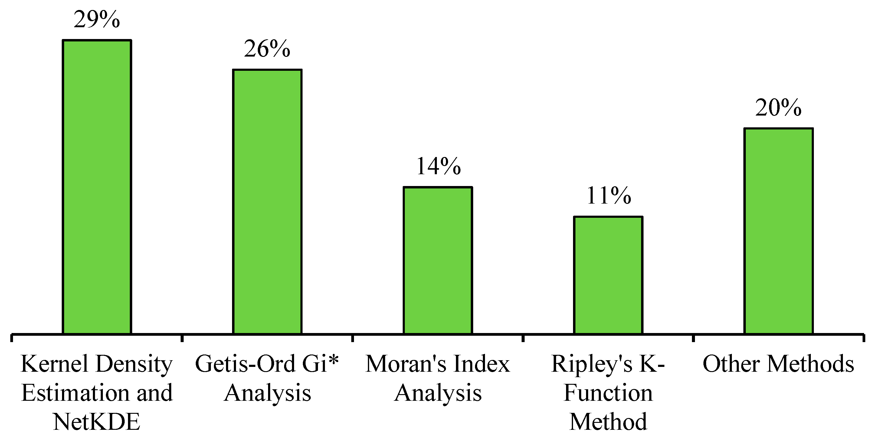
Figure 1. Comparison of Euclidean Distance and Network Constraint Distance.
Safety 09 00057 g001
Figure 2. Overview of Past Methodologies and Workflows.
Safety 09 00057 g002
Figure 3. Spatial Analysis Methods Used in the Reviewed Literature.
Safety 09 00057 g003
Figure 4. Road Network Map of the Study Area with Crash Locations.
Safety 09 00057 g004
Figure 5. Analytical Workflow.
Safety 09 00057 g005
Figure 6. Pattern analysis of vulnerable road user crashes using the (a) G-function and (b) K-function.
Safety 09 00057 g006
Figure 7. Gi* hot and cold spots using thresholds based on (a) the network travel distances, and (b) Euclidean distances based on Moran’s I.
Safety 09 00057 g007
Figure 8. Comparison of Getis-Ord Gi* based on G-function and Moran’s I, (A) injury severity proportions in Hot Spots, (B) injury severity proportions in Cold spots.
Safety 09 00057 g008
Figure 9. Gi* hot and cold spots using network-constrained threshold distances based on the G-function (AC), and Euclidean distances based on Moran’s Index (DF).
Safety 09 00057 g009
Figure 10. Fatal Crashes hot and cold spots (Scenario 1: G-function based, Scenario 2: Moran’s I based).
Safety 09 00057 g010
Figure 11. Crash Severity of Significant Spots based on threshold distance of Moran’s I and G-function.
Safety 09 00057 g011
Figure 12. Crash prediction accuracy evaluation (a) Cross-K-function “Scenario-1”, (b) Cross-G-function “Scenario-1”, (c) Cross-K-function “Scenario-2” and (d) Cross-G-function “Scenario-2”.
Safety 09 00057 g012
Table 1. Summary of Methods Used in Reviewed Literature.
MethodArticlesProsCons
1.Kernel density estimation[26,33,35,38,39,45,46,47,48]KDE can be employed to visualize crash densities across various geographical regions. The smoothness of the density surface is conditional upon the careful selection of the appropriate bandwidth. Network-Constrained KDE offers an enhanced level of accuracy by providing route-specific density information.KDE results are overly sensitive to the choice of bandwidth. The resulting density estimates can exhibit variations when different kernel shapes are employed, for example, Gaussian, Epanechnikov. Furthermore, the computational process might become demanding, especially when dealing with larger geographical areas and more extensive datasets and network constrained estimation.
2.Getis-Ord Gi*[11,19,21,22,26,34,35,36,42,48]Getis-Ord Gi* effectively identifies clustering patterns of high-high or low-low values. High-high clusters, known as hot spots, are characterized by a highz-score and a small p-value. Conversely, low-low clusters, referred to as cold spots, involve a low negativez-score and a small p-value.The Gi* statistics are sensitive to the choice of threshold distance. Moreover, employing various distance methods (such as Manhattan, Euclidean, or actual network distance) can yield divergent outcomes. Hence, it is crucial to opt for an appropriate distance method to establish accurate spatial relationships.
3.Moran’s Index[11,19,21,22,36,47]Moran’s Index is used to identify the clustering or dispersion in data based on spatial autocorrelation supported byz-score and p-value. The null hypothesis used in Moran’s Index is that “the values of the features are spatially uncorrelated” [49]. Using the Incremental Spatial Autocorrelation tool, a threshold distance to be used in Local Moran’s I and Getis-Ord Gi* analysis is calculated. Similar to Getis-Ord Gi*, Local Moran’s I is also influenced by scale and sensitive to a threshold distance, which can be identified in advance through the Incremental Spatial Autocorrelation method or the method we are proposing in this research, i.e., K-function and G-function method. Furthermore, inappropriate distance method selection may lead to an inaccurate Moran’s I result.
4.Ripley’s K-function[11,26,38,42,50]Ripley’s K-function is used to identify spatial patterns of data (clustering, dispersion, or randomness). K-function can be used on both local and global scales. A network restraint K-function provides more accurate results in case of crash data. Additionally, the K-function enables the comparison of spatial patterns between two distinct datasets.Unlike Moran’s I, K-function lacks consideration of attribute values, thus not providing insights into the underlying causes of spatial patterns. Similar to Getis-Ord Gi* and Moran’s I, Ripley’s K-function results are also dependent on the type of distance method used. The calculation process may be computationally extensive in cases of network restraint Ripley’s K-function.
5.Other methods[42,43,44,45,46,47,51]--
Table 2. Proportions of Severity Levels in the Training Dataset.
Severity LevelKABCO
Scale [54]
2017–20192020–2021
BikesPedestrianTotal (%)BikesPedestrianTotal (%)
Fatal CrashK54651 (1.30%)21820 (1.20%)
Injury (Severe)A106299405 (10.6%)54160214 (12.6%)
Injury (Other Visible)B5857361321 (34.6%)269329598 (35.3%)
Injury (Complaint of Pain)C69813412039 (53.4%)309552861 (50.9%)
Total 139424223816 (69.3%)63410591693 (30.7%)
Table 3. Advantages of Using Ripley’s K-/G-Function and Moran’s Index Method.
Ripley’s K- and G-FunctionMoran’s Index:
Advantages:
  • Detection of different types of spatial patterns: Both the K- and G-functions can detect clustering as well as the dispersion in point patterns.
  • Versatility: Both the K- and G-functions can be applied to a wide range of datasets, including both continuous and categorical variables.
  • Scale-invariance: These methods are scale-invariant, meaning that the results will not be affected by changes in the scale of the data.
  • Multi-scale analysis: Both the K-and G-functions can be used to study spatial patterns over multiple scales, unlike Moran’s Index.
  • Topology: Network Constrained K-and G-function application available using R-Package (SpNetwork).
Advantages:
  • Simplicity: The method is easy to understand and calculate, making it accessible to a wide range of users, including those with limited statistical expertise.
  • Flexibility: Moran’s Index can be applied to a wide range of datasets, including both continuous and categorical variables.
  • Interpretability: The resulting index can be interpreted straightforwardly, with positive values indicating clustering and negative values indicating dispersions.
Table 4. Disadvantages and Limitations of Using Ripley’s K-/G-Function and Moran’s Index Method.
Ripley’s K- and G-FunctionMoran’s Index:
Disadvantages and Limitations:
  • Complexity: Both the K- and G-functions are more complex to understand and calculate than Moran’s Index and may require more advanced statistical expertise.
  • Computationally intensive: These methods can be computationally intensive, particularly when dealing with large datasets.
  • Assumptions: Both the K- and G-functions make assumptions about the underlying point process, such as the assumption of complete spatial randomness (CSR). If these assumptions are not met, the results may not be reliable.
  • Not sensitive to outliers: Both the K- and G-functions are not affected by outliers in the data, unlike Moran’s Index.
Disadvantages and Limitations:
  • Sensitivity to outliers: The method can be sensitive to outliers in the data, which can affect the overall index value and make it difficult to interpret.
  • Limited discrimination: Moran’s Index is only able to detect overall spatial autocorrelation and is not able to distinguish between different types of spatial patterns such as clustering or dispersion.
  • Scale dependence: The method is typically only used to study patterns at the local scale and does not consider spatial patterns at larger scales. It should be noted here that Global Moran’s Index provided an assessment of the overall spatial distribution of point data observations.
  • Assumptions: Moran’s Index method has certain assumptions such as normality and stationarity of the data, if these assumptions are not met, the results may not be reliable.
Disclaimer/Publisher’s Note: The statements, opinions and data contained in all publications are solely those of the individual author(s) and contributor(s) and not of MDPI and/or the editor(s). MDPI and/or the editor(s) disclaim responsibility for any injury to people or property resulting from any ideas, methods, instructions or products referred to in the content.

