Levee System Reliability Modeling: The Length Effect and Bayesian Updating

Abstract

In levee system reliability, the length effect is the term given to the phenomenon that the longer the levee, the higher the probability that it will have a weak spot and fail. Quantitatively, it is the ratio of the segment failure probability to the cross-sectional failure probability. The literature is lacking in methods to calculate the length effect in levees, and often over-simplified methods are used. An efficient (but approximate) method, which we refer to as the modified outcrossing (MO) method, was developed for the system reliability model used in Dutch national flood risk analysis and for the provision of levee assessment tools, but it is poorly documented and its accuracy has not been tested. In this paper, we propose a method to calculate the length effect in levees by sampling the joint spatial distribution of the resistance variables using a copula approach, and represented by a Bayesian Network (BN). We use the BN to verify the MO method, which is also described in detail in this paper. We describe how both methods can be used to update failure probabilities of (long) levees using survival observations (i.e., high water levels and no levee failure), which is important because we have such observations in abundance. We compared the methods via a numerical example, and found that the agreement between the segment failure probability estimates was nearly perfect in the prior case, and very good in the posterior case, for segments ranging from 500 m to 6000 m in length. These results provide a strong verification of both methods, either of which provide an attractive alternative to the more simplified approaches often encountered in the literature and in practice.

1. Introduction

The length effect was first brought to light by Leonardo de Vinci, who said “Among cords of equal thickness the longest is the least strong” [1]. In the context of levees, the length effect refers to the fact that as the length increases, there is a larger distance over which to encounter a weak spot in the levee, and thus a higher probability of failure. Typical reliability analyses of levees compute the probability of geotechnical failure over a small or infinitesimal length referred to as a cross section. However, risk analysis is often interested in the failure probability of long stretches (or reaches) of levees. Depending on the spatial variability of the soil parameters, and the length of the levee, the failure probability of a reach can be many times greater than that of a cross section. Incorrectly assigning it to the reach can lead to inaccuracies in failure and risk assessment of levees, in an unconservative direction.

Different approaches of accounting for the length effect in levees can be found in the literature. Vanmarcke proposed a method involving first crossings [2,3] to estimate the probability of failure over a longitudinal length. A crossing refers to the resistance being surpassing by the load, or equivalently the difference between them (also referred to as the limit state function) crossing zero and becoming negative. The method calculates the probability of such a crossing along a given length. It treats the limit state function as a random field, the parameterizing of which requires some assumptions. Li and Hicks [4] compared a simple reliability method for long earthen slopes proposed by Vanmarcke [5] with a fully three-dimensional model for slope stability and concluded that for large scales of fluctuation, the methods were in agreement, but for small scales of fluctuation, the Vanmarcke approach can produce unconservative reliability indices. The slope they considered was only 50 meters long, so the differences may have been due predominantly to the simplified modeling of slope instability in the Vanmarcke method, rather than the method of handling the spatial variability. More pragmatic methods are also found in the literature. Bowles et al. [6] took the length effect into account in a risk analysis of the Herbert Hoover Dike in Florida. In that case, they broke up the levee into segments of about 500 m, and for all failure mechanisms besides ’piping through the foundation’, they assumed the segments were independent. For piping through the foundation, they judged that there was ‘some correlation’ between sections, and accounted for this by taking the average of failure probability assuming (1) full correlation and (2) complete independence. This approach does not clarify for which correlation such an average is valid, or how likely that correlation is to be the correct one. The risk methodology manual developed by the U.S. Bureau of Reclamation [7] contains guidance for the length effect, proposed by the U.S. Army Corps of Engineers. Essentially they break up segments into ‘characteristic lengths’ which can be considered statistically independent. They do not specify how to estimate the characteristic length other than stating that it can be based on statistical analysis of spatial correlations, or via expert judgment.

In the Netherlands, a modified version of the standard outcrossing method is used to calculate the length effect, which we refer to in this paper as the modified outcrossing (MO) method. It is programmed into the flood defense reliability model Hydra-Ring (based on a previous model PC-Ring) [8,9] that is used in national flood risk studies [10,11,12] and to support the assessment of flood defenses. Reliability calculations are often concerned with limit state functions, which are defined to be negative when geotechnical failure (such as piping or slope instability) occurs, and positive otherwise. The MO method approximates the limit state function as a one-dimensional Gaussian random field. This follows directly when first-order reliability method (FORM) is used at the cross section level, because FORM approximates the limit state function as a linear combination of Gaussian processes. However, it is not required to use FORM at the cross-section level; if, for example, Monte Carlo is used, the design point (the most probable set of variables leading to failure) can be estimated and used to approximate the limit state function as a linear combination of Gaussian processes. The MO method then uses the theory of outcrossing rates for Gaussian and ergodic random fields to determine the probability that the limit state becomes negative for at least one point along the levee segment. The MO method is similar to that of Vanmarcke [2,3], but is modified to handle the non-ergodicity of the limit state function. Information about the MO method can be found in [8,9,13,14], and we provide details in Appendix A. Parallel research is looking into theoretical details of the MO method and its effect on design codes for flood defense systems [15]. One of the issues we address in this paper is that although the MO method is an integral part of national flood risk analysis in the Netherlands, its accuracy has not been tested.

In this paper, we propose a method to compute the length effect by sampling from the (discretized) joint spatial distribution of the limit state function, using a copula approach. A similar approach has been proposed in other areas of engineering [16], but has not been applied to levee reliability. We represent the joint distribution with a Bayesian network (BN), which allows us to visualize the correlation structure in the joint spatial distribution, and clarifies how the different parts of the reliability analysis fit together. Using the BN, we are able to update the joint distribution using observations. In this paper, we focus on updating the reliability estimate using survival observations. These are coupled observations of a (high) water level and survival of the levee, which we have in abundance. Researchers have looked at updating reliability estimates at a cross-section scale [17]. In this paper, we expand upon this by using the BN to update the reliability of a (long) levee segment.

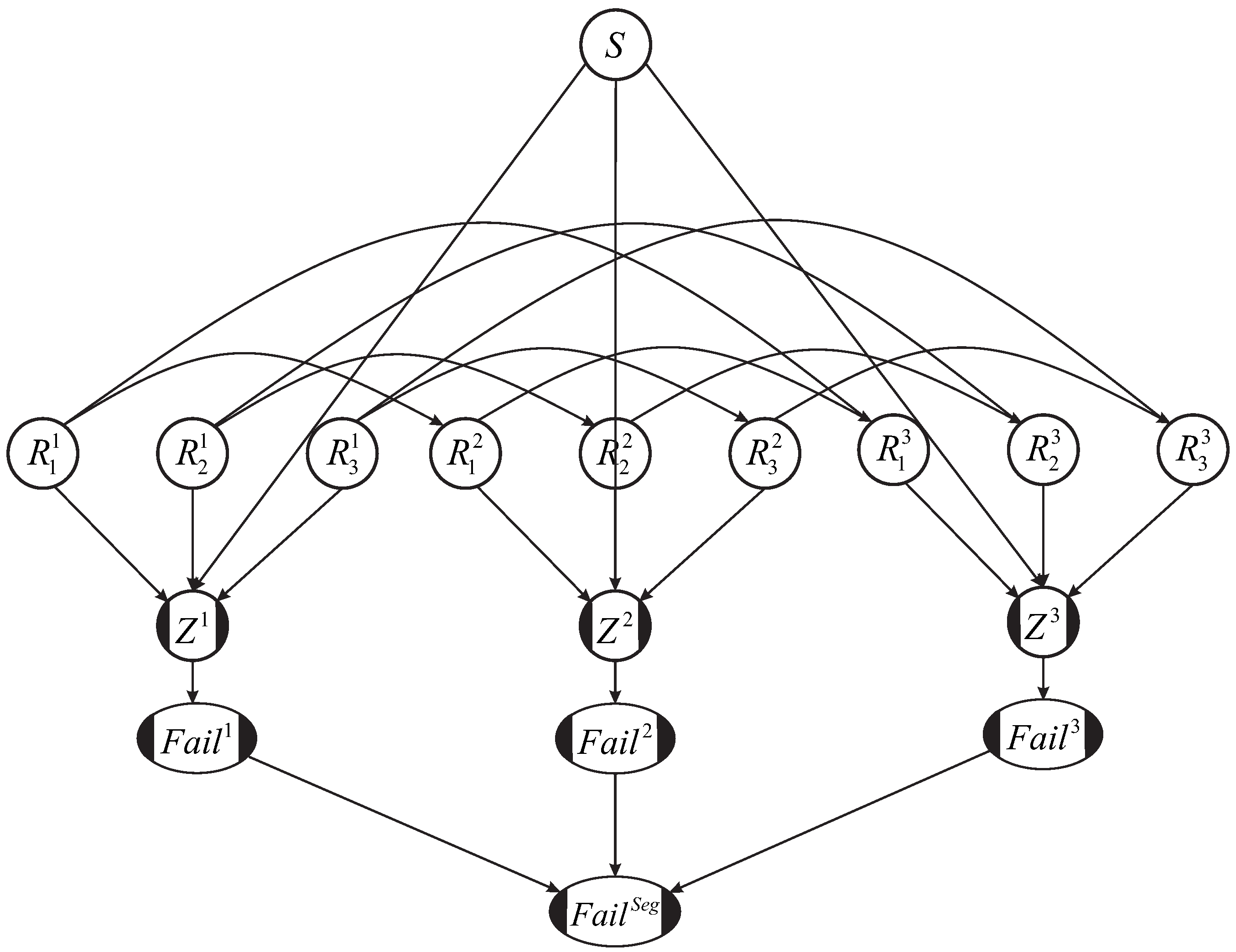
Traditional Bayesian networks, which work with inference algorithms designed for discrete distributions, become severely burdened computationally when the BN is densely connected (i.e., lots of correlations between variables). This is the case in levee reliability where the soil parameters are spatially correlated. When we slice up the levee into cross-sections (i.e., discretize the random field), the resistance variables in one cross section will be correlated with (connected to) the resistance variables in all other cross sections. Bensi et al. [18] developed an approximate method to make discrete BNs tractable in these cases, but it remains difficult to know apriori how much error will be incurred for a particular application. Further, they require discrete conditional probability tables. In levee reliability applications, we generally have continuous marginal distributions of the random variables, where we are particularly interested in the tails of the distributions. The method we propose in this paper is particularly well-suited to levee reliability problems. It allows variables in the network to be described by continuous marginal distributions; correlations between variables are captured via autocorrelation coefficients. It assumes a Gaussian autocorrelation structure of resistance variables, but—in contrast to the MO method—does not approximate the limit state function as a Gaussian random field. Note that in general the limit state function is not a Gaussian random field because it is an (often non-linear) combination of resistance and load variables that are traditionally not Normally distributed (note that the terms “Normal” and “Gaussian” are used interchangeably throughout the paper).

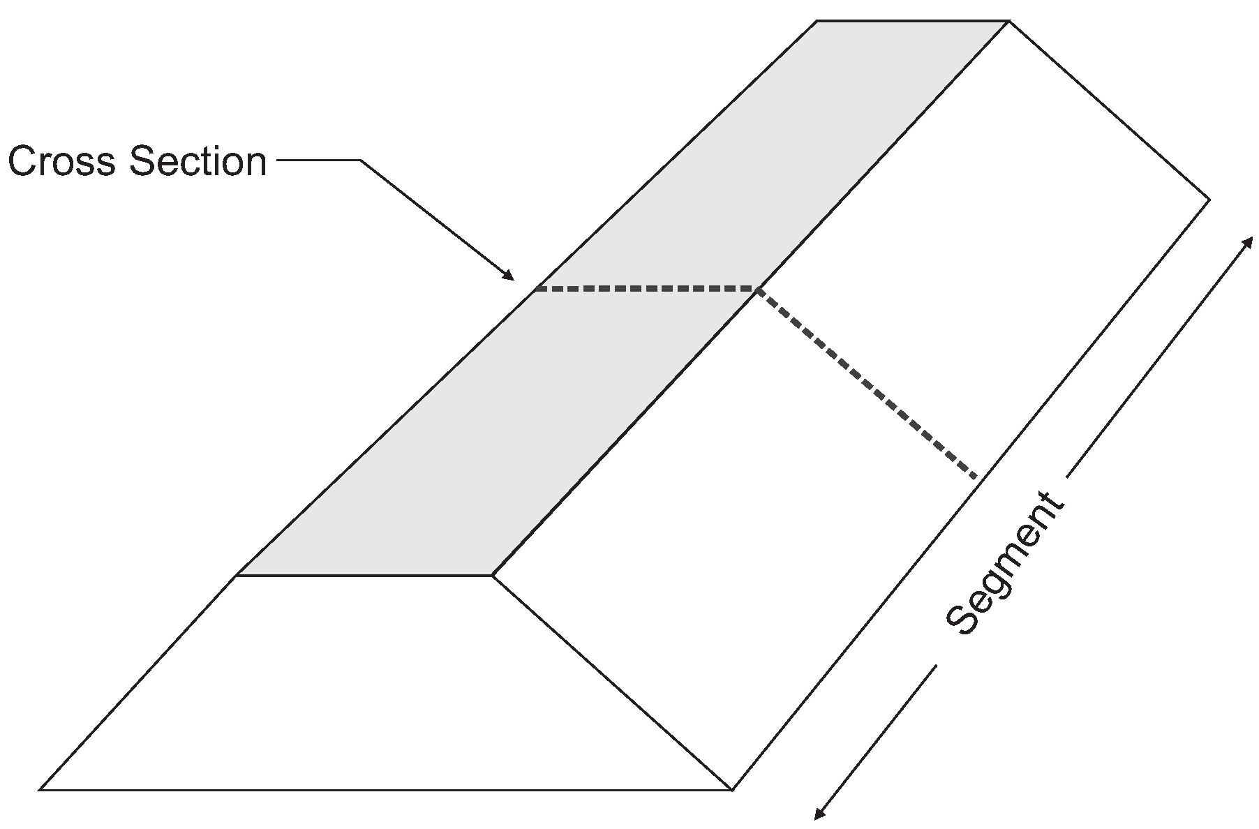
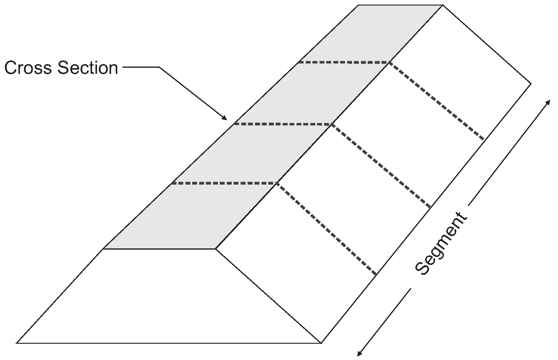
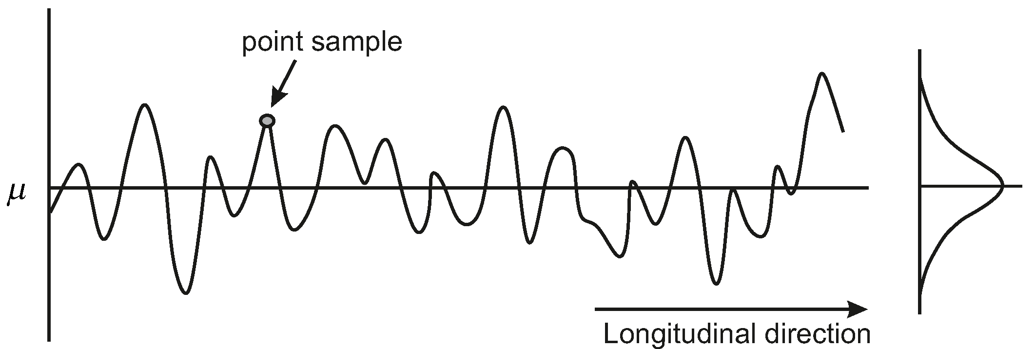
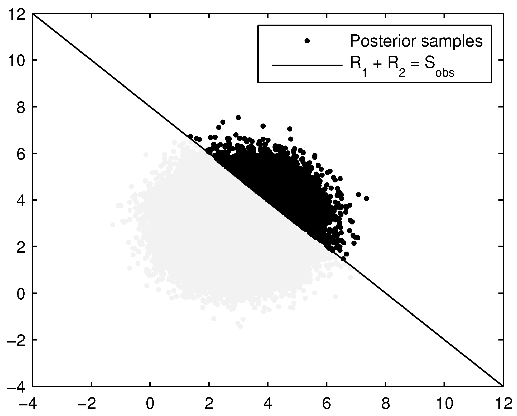
The spatial scales we consider in this paper are a cross section (typically in the order of meters) and a statistically homogeneous levee segment (order of kilometers). Figure 1 shows a schematic of a levee segment and a cross section. Computing levee reliability often relies on failure mechanism models, which calculate whether a particular failure mode—such as geotechnical stability or piping—will occur given specific soil properties and load conditions. The random variables in these models sometimes take into account some degree of spatial averaging over the vertical dimension of the levee (e.g., slope stability), but the reliability estimate is only valid for a relatively short length of the levee (i.e., a cross section). This is because the mechanism models generally look at point values of the soil parameters, while in reality these parameters are random fields over the length of the segment. Consider Figure 2; for a given point sample, there is the possibility of many other values of the soil parameter at other locations along the segment, even though they are all governed by the same probability distribution (see right side of Figure 2). To estimate the failure probability of the segment, we need to account for the spatial variability of the soil parameters and the likelihood of finding a weak spot in the segment.

This paper has two main objectives: The first is to present the proposed BN method for computing the length effect in levee reliability, and the second is to use the BN method to address the accuracy/validity of the MO method, both with and without reliability updating using survival observations. The BN method is considered a more exact method (provided enough Monte Carlo samples are taken) because it does not require any assumptions about the distribution or correlation function of the limit state function (which the MO method does). We also devote attention to comparing the computational efficiency of the two methods, and exploring under which conditions survival observations are most informative. Section 2 provides a brief background about the MO method (detailed information is provided in Appendix A; in Appendix B, we describe how we updated the segment failure probability—based on a survival observation—using the MO method). Section 3 presents background about BNs, and introduces a new method for computing the reliability of a levee segment using a BN, as well as updating the reliability using a survival observation. Section 4 presents a numerical example via which we compare the BN and MO methods, both prior to and following the incorporation of a survival observation. Section 5 provides discussion about (1) the influence that the prior failure probability and the extremity of an observed load have on the impact of a survival observation, and (2) computational costs of both the BN and MO methods. Section 6 presents general conclusions.

2. Modified Outcrossing Method

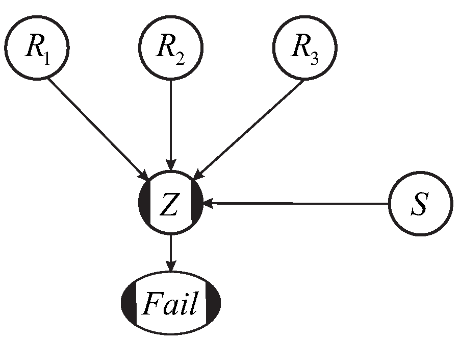
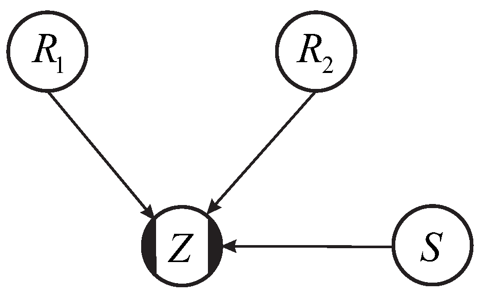
The modified outcrossing (MO) method to compute the failure probability of a homogeneous levee segment begins by computing the failure probability of a cross section, $P_{f,CS}$. While not required, this cross-sectional failure probability is typically calculated using first order reliability method (FORM) because it returns influence coefficients of the random variables, which we will need (see below). The limit state function (Z) depends on load and resistance variables (denoted later in the paper by S and R, respectively). In the MO method the loads and resistances are approximated as Gaussian processes, and the limit state as a linear combination of them (and thus itself also a Gaussian process). That is, the limit state function can be written as $Z=\beta +{\alpha }_1{U}_1+{\alpha }_2{U}_2+\dots +{\alpha }_n{U}_n$, where $U_i$ is the i-th standard-Normally-distributed load or resistance variable, and ${\alpha }_i$ is its influence coefficient. The reliability index $\beta$ is directly related to the failure probability: $\beta =-{\mathsf{\Phi }}^{-1}\left(P_{f,CS}\right)$, where ${\mathsf{\Phi }}^{-1}$ is the inverse standard Normal distribution. Z can be written equivalently, but more compactly, in the form of Equation (1), where U is a standard Normally distributed variable. The spatial autocorrelation of Z is modeled according to Equation (2), where $\Delta x$ is the longitudinal distance between two points, $d_x$ is known as the correlation length, and dictates how quickly the correlation decreases in space, and ${\rho }_x$ is the residual correlation at large distances. Note that in Equation (2), ${\rho }_x$ represents the non-ergodic part of the autocorrelation. Expressions for $d_x$ and ${\rho }_x$, which depend on the autocorrelations and influence coefficients of the load and resistance variables, are available in the literature [9,13], and are provided in Appendix A.

$$Z=\beta -U$$

(1)

$${\rho }_Z\left(\Delta x\right)=\left(1-{\rho }_x\right)exp\left(-\frac{\Delta x^2}{d_x^2}\right)+{\rho }_x$$

(2)

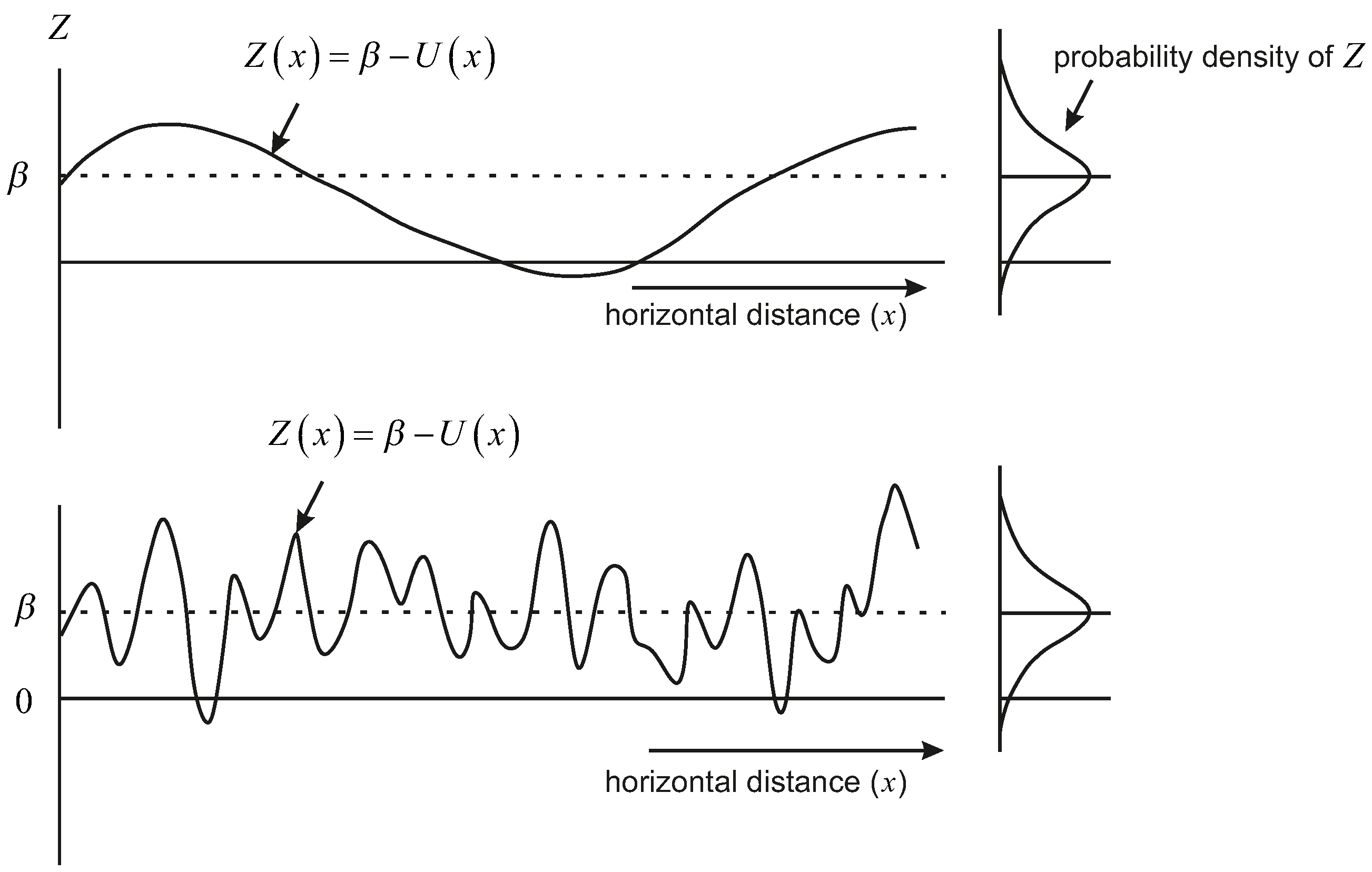
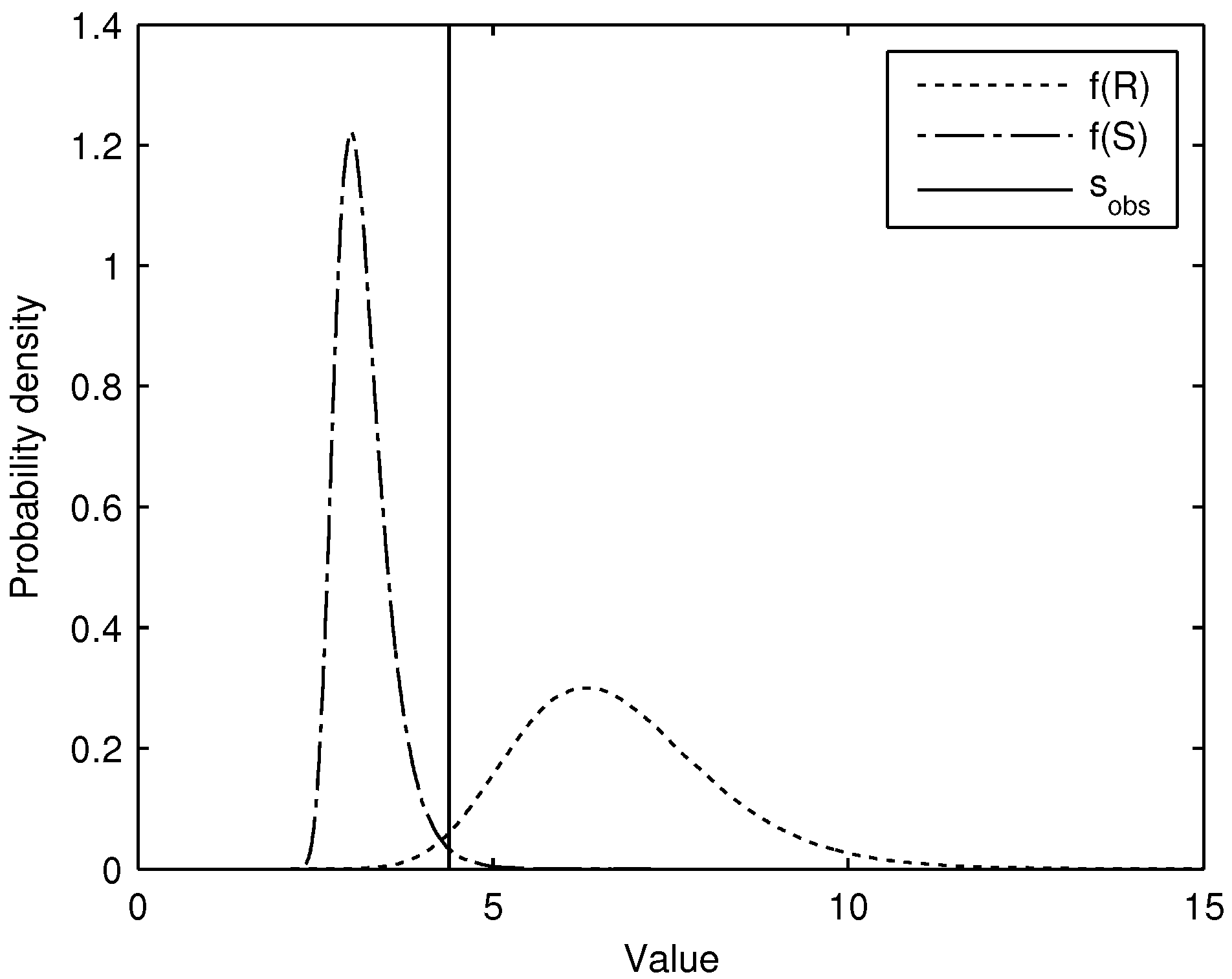
Figure 3 illustrates the limit state function Z as a random field in one dimension (longitudinally). The probability of having a realization for which $Z<0$ increases as the length of the segment increases. The increase is dependent on both the length of the levee (L), and how frequently Z crosses 0. This latter quantity is referred to as an outcrossing rate, and is dependent on the spatial autocorrelation of Z. For example, as seen in Figure 3, a strongly-autocorrelated Z function will change slowly in space, while a weakly-autocorrelated Z function will show much more rapid change (allowing more opportunities for Z to cross 0). The strength of the autocorrelation between two locations is dictated by the correlation length $d_x$ in Equation (2).

The outcrossing rate is calculated analytically based on theory for Gaussian ergodic random fields (see Van Marcke [3]). However, the limit state function is not ergodic, due to the nearly fully-correlated nature of the load over a levee segment (other variables which are fully correlated over the length of the levee segment (such as model uncertainty) also contribute to the non-ergodicity of the limit state function). This is taken into account by calculating the segment failure probability conditional on the non-ergodic part of the limit state function, and then using the theorem of total probability to obtain the full segment failure probability.

Full details of the MO method are provided in Appendix A. Appendix B presents the details of how the MO method was applied in this paper when updating with survival observations (this has not been done in practice, and we were required to make some choices in our implementation for this paper).

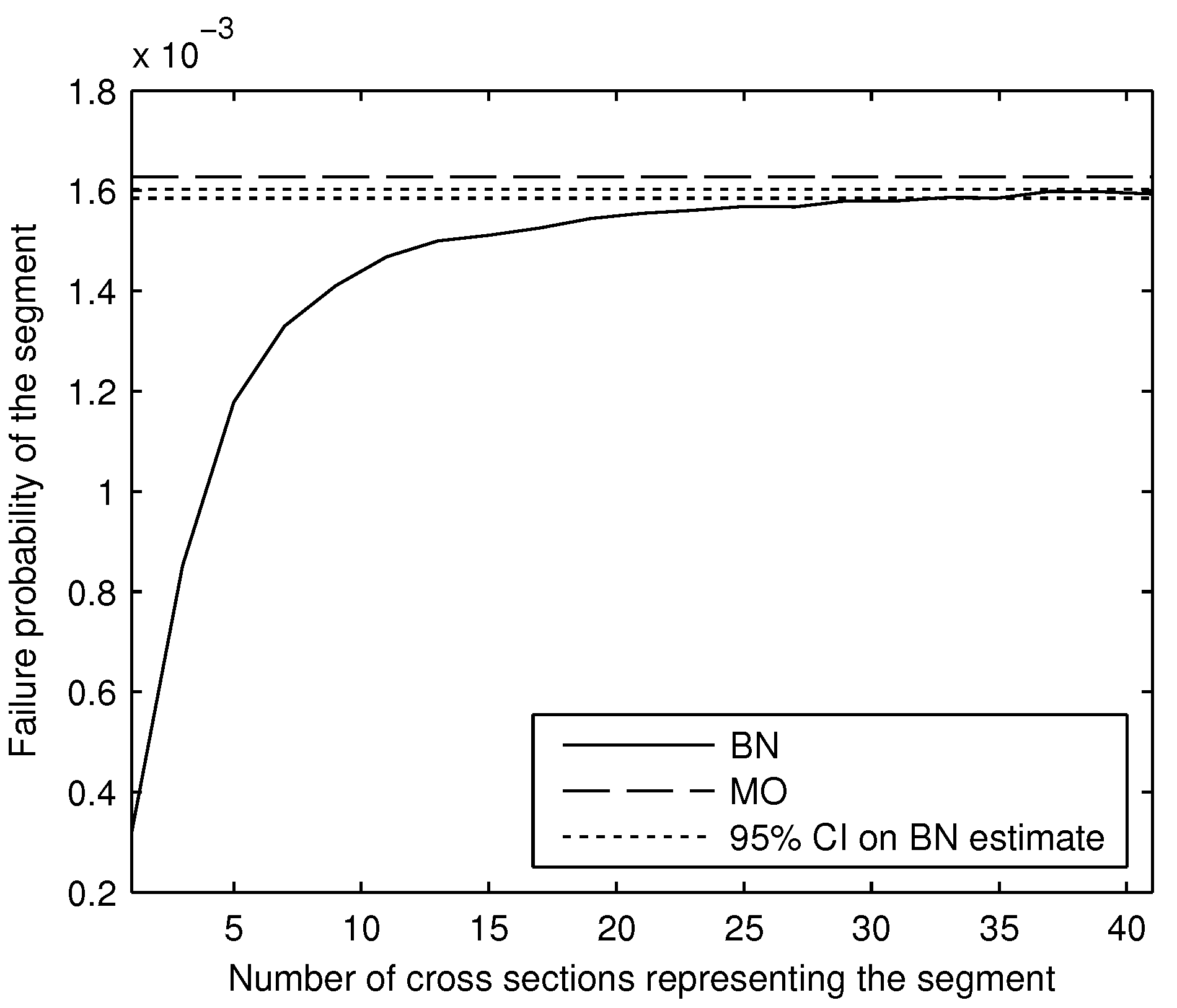
In this paper, we are interested in verifying the MO method, which relies on the approximation of Z as a Gaussian random field. The marginal distribution of Z is modeled as a Normal distribution, and a Gaussian correlation structure is assumed. In general, the limit state function is not a Gaussian random field, because it is an (often) nonlinear combination of variables which are not necessarily Normally distributed. It is unclear how well the approximation works, both prior to and following incorporation of a survival observation. In the next section we describe a method to compute the failure probability of a levee segment in which the (discretized) spatial joint distribution of the resistance variables—and the limit state function—is represented by a BN, and sampled using a copula approach. Because the BN method does not require the limit state function to be approximated by a Gaussian random field, we can use the failure probability estimates from the BN to evaluate the accuracy of the prior and posterior failure probabilities computed by the MO method.

3. Bayesian Network Approach

3.1. Background

A Bayesian network (BN) is a type of probabilistic graphical model; it is a graphical way to describe a multivariate joint distribution. BNs are particularly convenient when the joint distribution is complex (involving many correlated variables), or when we want to update the estimate of the joint distribution once one or more of the variables in the network have been observed. The traditional approach to a BN is to is to factorize the joint distribution into marginal and conditional distributions, using the graphical structure to identify the needed conditional distributions (according to the arcs between the variables). BNs can represent joint continuous distributions; however, their most common form is in the discrete domain, where distributions are tabulated, i.e., conditional distributions are represented by conditional probability tables. Figure 4 presents a simple example; variables are represented by circular nodes, and arcs (arrows) between nodes represent dependence. For example, in Figure 4 the independent variables $X_1$ and $X_2$ are referred to as the parents of $X_3$, and variable $X_3$ is referred to as the child of $X_1$ and $X_2$. Each node is assigned a conditional probability table, conditional on its parents. Nodes without parents are described by marginal probability tables. The joint distribution is the product over all of the node probabilities. Equation (3) shows the joint distribution represented by this example network.

$$P\left(X_1,X_2,X_3\right)=P\left(X_1\right)·P\left(X_2\right)·P\left(X_3|X_1,X_2\right)$$

(3)

BNs can contain nodes that have a functional relationship (i.e., described by formulas) with their parents. Such nodes are referred to as functional nodes.

The BN described above suffers two shortcomings when it comes to reliability analysis: (i) Efficient inference algorithms are almost exclusively available for discrete distributions, while in reliability analysis we typically have continuous distributions, and are particularly interested in the tails, and (ii) all dependent (i.e., child) nodes must be represented by conditional distributions, while we typically have marginal distributions, which we can obtain from data. Hybrid BNs address the first of these, allowing nodes to be described by both discrete and continuous distributions. A number of these have been developed [19,20,21], and often involve discretization, which has drawbacks [19]. The method we use falls under a type of network known as a non-parametric hybrid BN, and allows for variables to be represented by marginal, continuous distributions. Details are provided in the following section.

3.1.1. Non-Parametric Hybrid Bayesian Network

The non-parametric hybrid BN [22,23,24] was developed to address some of the shortcomings in traditional networks. A good comparison with other hybrid networks, as well as more recent applications using the non-parametric hybrid BN, are provided in [25]. The name ‘non-parametric’ is a bit misleading, but is meant to emphasize the fact that no parametric form of the joint distribution is necessary. It describes nodes in the network with marginal distributions (which can be parametric, though not required), and calculates the dependence structure among the variables using copulas.

Copulas were first introduced by Sklar [26] as a convenient way to build multivariate probability distributions, because they separate the dependence structure from the marginal distributions. The word “copula” means “link” in Latin, and copulas literally link the marginal distributions together to form the joint distribution. Suppose we have a random vector $X=(X_1,...,X_n)$, with marginal distribution functions $F_1,...,F_n$, and a joint distribution function $F_{1,...,n}$. A copula C is a joint distribution function that operates on uniform random variables, and satisfies Equation (4).

$$F_{1,...,n}\left(X_1,\dots ,X_n\right)=C\left(F_1\left(X_1\right),\dots ,F_n\left(X_n\right)\right)$$

(4)

There are many popular copulas, which differ most notably in how they describe tail correlation (see [27,28]). The choice of copula is usually determined by observing the tail dependence in data. The non-parametric BN can theoretically take any copula to represent the dependence structure, but using the Gaussian copula makes performing inference more efficient. This is because the Gaussian copula inherits most of the properties of the Gaussian distribution, which in turn allows for analytical derivations of any conditional distributions.

In reliability analysis, it is common to use the Nataf or Rosenblatt transformation to describe and sample correlated variables. It has however been shown that the classic version of Nataf and the Rosenblatt transformations are equivalent to using the Gaussian copula (see [27,29]), which we use in this paper. The practical implementation we used is to sample [$U_1,...U_n$] from the multivariate standard Normal distribution ${\mathsf{\Phi }}_{\Re }\left(\mathbf{0},\Re \right)$, where $\mathbf{0}$ is an $n\times 1$ vector of means equal to zero, and ℜ is the $n\times n$ linear correlation matrix, which in the case of the (multivariate) standard Normal distribution is equal to the covariance matrix. The variables $[X_1,...,X_n]$ are then derived using their inverse marginal distributions: $X_i=F_i^{-1}\left(\mathsf{\Phi }\left(U_i\right)\right)$, where $\mathsf{\Phi }$ is the standard Normal distribution function.

The use of the Gaussian copula requires a positive definite correlation matrix. In our application, this is guaranteed because we use a positive definite correlation function to generate the autocorrelations. In general though, where the joint distribution is over many variables, with correlation information coming from any combination of judgment or data, it can be impossible to intuitively construct a positive-definite correlation matrix. In these cases, the non-parametric BN is particularly helpful, because it allows the specification of conditional rank correlations (the parameters of the conditional copulas), which can be anything between −1 and 1, and transforms these into a unique, valid positive-definite correlation matrix, using recursive formulas provided in [30].

The use of copulas, and the ability to work with conditional rank correlations, while still guaranteeing positive definiteness, make the non-parametric BN a powerful tool to sample from complex, non-parametric joint distributions. It also performs both forward inference (when input variables are observed) as well as backward inference (when output or functional variables are observed), making it particularly useful in cases exploring the impact of good performance of a structure, under known loading conditions. We discuss the specifics of how inference is performed in Section 3.3.

3.2. Modeling Levee Reliability with a Bayesian Network: Methodology

We describe in this section how we model levee reliability at different spatial scales. The method is presented for the case that failure of the levee is described by a formula. In these cases, the limit state function is represented by a functional node. BNs can be excellent tools in cases where the failure mechanism is not analytically formulated. However, it would require some preprocessing, and falls outside the scope of this paper. Specifically, the geotechnical model describing failure would need to be used to extract the dependence between the input random variables and the output variables (e.g., the limit state function). The latter would then be incorporated within the BN as a non-functional random variable, with arcs and correlations representing the dependence extracted via the geotechnical model (see [31] for an example). Thereafter, the method as presented in this paper could be applied.

3.2.1. Reliability of a Levee cross Section

We begin by considering the reliability of a cross section. We build the BN based on the formulaic representation of failure, which is often postulated as a limit state function. We include a failure node in the network, $Fail$, which is binary: 0 when $Z\ge 0$ and 1 when $Z<0$. In the MO method, the limit state is recast into a standardized form (see Section 2). In the BN, we describe the limit state as a function of the load and resistance variables. As an example, consider a limit state function that depends on three resistance variables $R_1$, $R_2$, and $R_3$, and a load variable S. Figure 5 shows what the BN for the failure probability of the cross section might look like. Variables $R_1$, $R_2$, $R_3$, and S are shown as clear circular nodes, representing random input variables, and Z and $Fail$ are shown as circular nodes with black edges, representing functional nodes (this is the notation used by the UniNet software (https://lighttwist-software.com/); we have adopted the same notation in this paper). Note that in this example, the input variables are independent of each other (no arcs between them), but this does not have to be the case.

The BN is sampled taking into account any defined correlations between variables (see Section 3.1.1 for details). The failure probability can then be estimated according to Equation (5).

$${\widehat{P}}_f=\frac{1}{N}\sum _{j=1}^{N}fai{l}_j$$

(5)

N is the number of samples, and $fai{l}_j$ is the value of the failure node $Fail$ (1 or 0) for the j-th sample.

3.2.2. Reliability of a Levee Segment

Homogeneous levee segments can be long, typically a few kilometers. The failure probability of a cross section is therefore a poor representation of the failure probability of the entire segment. So instead of representing the failure probability by a single cross section, we represent it by multiple cross sections, and take care to honor the spatial autocorrelation of the variables between cross sections. Figure 6 shows an example of a levee segment whose spatial variability is represented by three cross sections. This can also be interpreted as splitting the segment into three sub-segments (where within a sub-segment there is full correlation), where the cross-sections represent the midpoint. Figure 7 shows what the BN would look like for the levee segment in Figure 6, for the case where the cross-sectional BN is described in Figure 5.

In the example in Figure 7, superscripts indicate the cross section. So for example, $R_1^2$ indicates variable $R_1$ in the second cross section. Similarly, $Fai{l}^1$, $Fai{l}^2$, and $Fai{l}^3$ represent the failure nodes for the first, second, and third cross sections, respectively. These cross-sectional failure nodes are then connected to a failure node for the entire segment, $Fai{l}^{Seg}$, a binary node (1 for failure and 0 for non-failure), described in Equation (6).

$$Fai{l}^{Seg}=\left\{\begin{array}{c}0,\mathrm{if}\forall iFai{l}^i=0\hfill \\ 1,\mathrm{if}\exists i\mathrm{s}.\mathrm{t}.Fai{l}^i=1\hfill \end{array}\right.$$

(6)

The number of cross sections needed to adequately estimate the failure probability of the segment will depend on the autocorrelation of the resistance variables, the length of the segment, and the magnitude of the prior failure probability. We iteratively increase the number of cross sections representing the segment, each time computing the failure probability of the segment, until additional cross sections no longer change the estimate. The method requires a defined stop criterion (e.g., a maximum difference in subsequent segment failure probability estimates), such that when the criterion is met, the number of cross sections is considered sufficient to represent the spatial variability of the segment. We discuss this in more detail with an example in Section 4.2.

We describe the arcs between resistance variables (see Figure 7) by Pearson product moment correlations. The latter can be estimated using data and one of a number of valid autocorrelation functions [32]. The one we use in this research is commonly used for resistance variables in the Netherlands [8,9,11], and depends on the distance between variables $\Delta x$ and a parameter $d_x$ which dictates how quickly the correlation decreases with distance; see Equation (7). This function is identical to the one used in the MO method for the limit state function (Equation (2)), for the case that the ergodic parameter ${\rho }_x$ is equal to zero. We exclude the parameter ${\rho }_x$ here because resistance variables (due to their heterogeneity) become uncorrelated at large distances.

$$\rho \left(\Delta x\right)=exp\left(-\frac{\Delta x^2}{d_x^2}\right)$$

(7)

Once we have specified the marginal distributions of the input random variables, the equations of the functional variables, and the correlation matrix $\Re =\left\{{\rho }_{jk}\right\}=\rho \left(\Delta x_{jk}\right)$ (see Equation (7)), where $\Delta x_{jk}$ is the distance between $R_i^j$ and $R_i^k$, we can sample the joint distribution as described in Section 3.1.1. We then enter these samples into the equations for the functional variables in the network, and derive the sample of $Fai{l}^{Seg}$. From this, we calculate the failure probability of the system using the standard Monte-Carlo estimator.

3.3. Inference

Inference is performed differently depending on the type of variable that is observed: An input variable or a functional one. An input variable is described by a marginal probability distribution, whereas a functional variable is described by an equation which operates on the input variables. In the sections below we describe how inference is performed for three cases: (1) An observed input variable, (2) an observed functional variable, and (3) a coupled observation of an input and a functional variable (e.g., observed water level and levee survival).

3.3.1. Observed Input Variable

When one or more input variables are observed, we can analytically compute the conditional joint Gaussian copula (conditional on the observed variable(s)). This is straight-forward and formulas are available; see ([30] (Section 2.4), and [33]). This is the power and benefit of using the Gaussian copula (note that it is also a feature of the multivariate Normal distribution in general). Once the conditional joint copula has been calculated, we can use the marginal distributions of each of the unobserved variables to translate back into real space.

3.3.2. Observed Functional Variable

When a functional variable is observed, we must first sample the network to perform inference. This generates an empirical joint distribution over the random and functional variables. We can then impose the observation as a constraint on the samples. For example, suppose we observe that the limit state function is greater than zero (indicating no failure): $Z>0$. We would then retain the joint samples of all our random variables for which $Z>0$, which would serve as an empirical conditional joint distribution. This is also known as rejection sampling, because we reject all samples for which our condition ($Z>0$) is not met. When the variance of the posterior failure probability estimate is too high using rejection sampling, other methods are available, such as importance resampling [34], or Markov-chain Monte Carlo [35], but we do not consider those in this paper.

3.3.3. Coupled Observation of Input and Functional Variables

Often we are interested in coupled observations of input and functional variables. Most notably in levee system reliability, we are interested in water level observations and the simultaneous failure/survival of the levee. These coupled observations allow us to update our failure probability estimate, and provide useful information about the remaining uncertain variables in the network.

In the case of coupled input and functional variables, we begin by first (analytically) specifying the conditional joint distribution, given the observed value of the input variable. Subsequently we sample the conditional joint network, and retain only those samples that meet the observed value(s) of the functional variable (e.g., $Z>0$ for survival). These retained samples form the updated empirical posterior joint distribution over the resistance variables.

3.3.4. Posterior Dependence

Observing the value of a variable in the network can introduce dependence between previously independent variables. This dependence is not always easily captured with a correlation coefficient. For example, consider a case where we have a limit state function $Z=R_1+R_2-S$, where $R_1$ and $R_2$ are resistance variables, and S is a load variable. This example is illustrated in Figure 8.

Now let us suppose that the load S is observed at $S=5$, and no evidence of failure was observed (i.e., $Z>0$). This means that $R_1+R_2>5$. Shown graphically (see Figure 9), we can see the dependence between the variables has a sharp boundary.

If one wants to use the updated distributions of the resistance variables for analysis, the posterior dependence between them must be accounted for. The simplest way to do this is to retain the posterior joint resistance samples. For example, in Figure 9, the posterior samples (shown as black dots) are retained for future analysis. It may be possible to develop a parametric way to represent such a constrained posterior dependence, but that was not explored in this paper.

3.3.5. Updated Failure Probability

The posterior segment failure probability $P_{f,seg}^{post}$ can be described by Equation (8). It is the probability that the spatial (multivariate) distribution $\mathbf{Z}$ is less than zero, given that at the time of the load observation ($t_{obs}$), $\mathbf{Z}$ was greater than zero (survival observed at time $t_{obs}$).

$$P_{f,seg}^{post}=P\left(\mathbf{Z}<0|\mathbf{Z}\left(t_{obs}\right)>0\right)$$

(8)

Our posterior distribution of the resistance variables includes the condition $\mathbf{Z}\left(t_{obs}\right)>0$, because we only retained joint samples for which this is the case. We therefore only need to calculate the probability that $Z<0$ using our joint posterior resistance samples. We sample the load S$N_p$ times (where $N_p$ is the number of posterior resistance samples), and calculate Z for each sample. Recall that the load is a temporally-spatial variable, and is unknown both before and after the observation time $t_{obs}$. The posterior failure probability is then calculated according to Equation (9).

$$P_{f,seg}^{post}=\frac{1}{N_P}\sum _{i=1}^{N_P}I\left(Z<0\right)$$

(9)

When computing the posterior failure probabilities, we are limited to the number of samples retained after performing inference. If this number is insufficient to keep the variance in the failure probability estimate low (this generally happens when the posterior failure probability is small), we use importance sampling, which is a method to reduce the variance in a MC estimate.

Importance sampling replaces the real distribution $f_S\left(S\right)$ with a biased one $g_S\left(S\right)$ that leads to a higher number of failures. The Monte Carlo output is weighted to correct for the use of the biased distribution $g_S\left(S\right)$ so that the failure probability estimate remains unbiased; see Equation (10) for the importance sampling estimator, wherein N is the number of samples, and $\mathrm{I}\left(·\right)$ is the indicator function.

$$P_{f,seg}=\frac{1}{N}\sum _{i=1}^N\mathrm{I}\left(Fai{l}^{Seg}=1\right)\frac{f_S\left(s_i\right)}{g_S\left(s_i\right)}$$

(10)

The choice of the biased distribution $g_S\left(S\right)$ will depend on the problem at hand. In general, for updating with survival observations, a reasonable choice is to translate the distribution $f_S\left(S\right)$ so that the mean is centered on the observed (high) load $S_{obs}$.

4. Numerical Example

In this section, we illustrate and compare the BN and the MO methods via a numerical example. We explore both prior and posterior failure probability estimates (the latter following from a specified coupled observation of load and levee survival) for levee segment lengths of 500 m, 1000 m, 2000 m, 4000 m, and 6000 m. This section is organized as follows: Section 4.1 provides details of the example, Section 4.2 describes the criterion we used to determine the number of cross sections in the BN, and Section 4.3 and Section 4.4 provide results and discussion about the prior and posterior failure probability estimates.

4.1. Details of the Example

We begin with the example we used for describing the posterior dependence among resistance variables, in Section 3.3.4, which considered a single cross section. The BN for the cross section was provided in Figure 8, and the limit state function describing cross-sectional failure is given in Equation (11). We assigned lognormal distributions to the resistance variables, $R_1$ and $R_2$, and a Gumbel distribution to the load variable S. These choices were made to mimic realistic cases, in which load variables are described by extreme value distributions (of which the Gumbel is one), and (soil) resistance variables are commonly described by lognormal distributions (in part due to the constraint that many soil parameters take on only positive values). The parameters of the resistance variables are provided in

Table 1. Lognormal distribution parameters $\mu$ and $\sigma$, distribution mean and standard deviation (SD), and correlation length $d_x$ for resistance variables $R_1$ and $R_2$.

Variable	Distribution	$\mathit{\mu }$	$\mathit{\sigma }$	Mean	SD	${\mathit{d}}_{\mathit{x}}$ (m)
$R_1$	Lognormal	0.842	0.385	2.50	1	200
$R_2$	Lognormal	1.420	0.232	4.25	1	200

and the parameters of the load variable in

Table 2. Gumbel parameters $\mu$ (location parameter) and $\beta$ (scale parameter), distribution mean and standard deviation (SD), and correlation length $d_x$ for variable S.

Variable	Distribution	$\mathit{\mu }$	$\mathit{\beta }$	Mean	SD	${\mathit{d}}_{\mathit{x}}$
S	Gumbel	3	0.3	3.8	0.15	∞

. The Gumbel probability density function is provided in Equation (12). We provide an illustration of the BN for the segment - using only three cross sections to keep the visualization clear—in Figure 10.

$$Z=R_1+R_2-S$$

(11)

$$f\left(x\right)=\frac{1}{\beta }exp\left[-\frac{x-\mu }{\beta }\right]·exp\left[-exp\left[-\frac{x-\mu }{\beta }\right]\right]$$

(12)

In this example, we consider survival of the levee for an observed load of $s_{obs}=4.38$, which corresponds to the 99% quantile of S (i.e. $P(S<s_{obs})=0.99$). We discuss the influence of the (extremity of the) load observation on the posterior failure probability in Section 5. The prior density functions of R and S are shown together with the observed load in Figure 11.

4.2. Number of Cross Sections in the BN

The criterion we defined for determining the number of cross sections to sufficiently represent the spatial variability of the segment (see Section 3.2.2 for a general description) is based on the width of the 95% confidence interval (this confidence interval captures the uncertainty due to the variance in Monte Carlo sampling) around the prior segment failure probability estimate, $P_{f,seg}$. We iteratively increase the number of cross sections representing the segment. To speed up the convergence we take two steps in the iterative process, so that $n=1,3,5,$ and so on, computing the segment failure probability estimate each time. We stop the iterative procedure when we find eight sequential iterations (e.g., $n=15$, $n=17$, ... , $n=29$) for which the estimates all lie within the 95% confidence interval of the last estimate. At this point, we consider the asymptote to have been reached, so that remaining differences between iterations are due only to sampling variance. The number of iterations for which the estimates must lie within the confidence interval—in our case eight—is somewhat arbitrary, and will require visual inspection of the results to confirm it is a good one.

The confidence interval around the failure probability estimate is computed according to Equation (13), and depends on the relative error $\epsilon$ of the segment failure probability estimate. The formula for the relative error (see reference [36]) is provided in Equation (14); it depends on the segment failure probability estimate, the number of Monte Carlo samples, N, and the value k, which is a quantile of the standard Normal distribution. So, for example, since we are interested in 95% confidence intervals, we would choose the quantile k such that $\mathsf{\Phi }\left(k\right)-\mathsf{\Phi }\left(-k\right)=0.95$, which is $k=1.96$.

$$CI=[(P_{f,seg}-\epsilon ·P_{f,seg}),(P_{f,seg}+\epsilon ·P_{f,seg})]$$

(13)

$$\epsilon =\sqrt{\frac{k^2}{N}\frac{\left(1-P_{f,seg}\right)}{P_{f,seg}}}$$

(14)

We determined the number of cross sections using the prior segment failure probability estimates, but applied it to both the prior and posterior BNs. In our case, this proved sufficient, but in general the same approach described above may need to be carried out separately for the posterior network if the prior number of cross sections seems insufficient to reach the posterior segment failure probability asymptote.

4.3. Prior Segment Failure Probabilities

We computed the segment failure probability with the BN and the MO method prior to incorporating any survival observations. Figure 12 shows (for the 1000 m levee segment) how the BN estimate of the segment failure probability increases with the number of cross sections that represent the segment, and the asymptotic behavior of the estimate once the number of cross sections meets the criterion discussed in Section 4.2. The confidence intervals around the BN estimate (shown in Figure 12) were calculated according to Equations (13) and (14). The MO estimate is also shown in Figure 12 for comparison; it is shown as a horizontal line because it is not a function of the number of cross sections in the BN.

The BN for the 1000 m segment was represented by 41 cross sections. The failure probability estimate is 0.0097 with confidence interval [0.0095, 0.0099]. The MO estimate is 0.0096. The results for the other segment lengths can be summarized by Figure 13. The BN and MO estimates are in near-perfect agreement, regardless of the length of the segment. The strong agreement between estimates is a good verification of both methods.

4.4. Posterior Segment Failure Probabilities

We are specifically interested in how well the MO method approximation holds when we take a survival observation into account (e.g., a simultaneous observation of water level and levee survival). The estimates for the failure probability of the 1000 m segment are presented in Figure 14. The agreement between the MO method and the BN remains very good. The BN estimates that $P_{f,seg}=1.59·{10}^{-3}$ and the MO method estimates $P_{f,seg}=1.63·{10}^{-3}$.

Figure 15 summarizes the posterior results for levee lengths of 500, 1000, 2000, 4000, and 6000 m. The differences between the MO and BN posterior segment failure probability estimates remain small, though they increase slightly as the length increases. For a 6000 m segment, the MO method estimates $P_{f,seg}=5.1·{10}^{-3}$ and the BN estimates $P_{f,seg}=4.6·{10}^{-3}$, which is a difference of about 10%. This is fairly minor, and in terms of reliability index $\beta$ (where recall $\beta ={\mathsf{\Phi }}^{-1}\left(1-P_{f,seg}\right)$), the difference is only $1\%$.

5. Discussion

In this section, we discuss (1) under which conditions survival observations are useful, as well as our choice of load in the numerical example, and (2) the computational costs of the BN and MO methods.

5.1. The Value of Survival Observations

In the example presented in Section 4, we considered an observed load equal to the 99% quantile of the load distribution. That is, the probability of observing a load higher than the observed load was $P(S>s_{obs})=0.01$. We chose this load because it is high enough that, together with a survival observation, it is likely to result in a valuable reduction in the failure probability estimate (though this will also depend on the prior segment failure probability, which we will discuss next). The other reason we chose this value of the load is that, while high, it is still realistic that we might observe it in measurement records.

We also considered in the numerical example a prior segment failure probability estimate of approximately $P_{f,seg}=0.01$. Failure probability estimates can be much lower, but if they are too low they are unlikely to benefit from a survival observation. For example, suppose the prior failure probability estimate is $P_{f,seg}={10}^{-4}$. Then even for a high load, such as the 99% quantile we just discussed, the expected conditional probability of failure at that load will still be very low. The observation that we did not see failure will therefore not be particularly informative in such a case.

Table 3. Reduction in the segment failure probability, computed as the ratio of prior to posterior segment failure probabilities, after updating with a coupled observation of the load ($s_{obs}$) and survival of the segment.

Prior ${\mathit{P}}_{\mathit{f},\mathbf{seg}}$	$\mathit{P}(\mathit{S}>{\mathit{s}}_{\mathbf{obs}})=0.1$	$\mathit{P}(\mathit{S}>{\mathit{s}}_{\mathbf{obs}})=0.01$	$\mathit{P}(\mathit{S}>{\mathit{s}}_{\mathbf{obs}})=0.001$
$0.01$	1.7	6.1	34.6
$0.001$	1.1	2.2	7.8
$0.0001$	1.0	1.2	2.2

shows the influence of both the extremity of the load and the prior segment failure probability on the impact of a survival observation, for the limit state we considered in the numerical example (see Equation (11)). The impact was measured as a reduction in the segment failure probability estimate, calculated as the ratio of the prior to posterior segment failure probabilities. In the table we consider three prior segment failure probabilities: $P_{f,seg}=0.01$, $0.001$, and $0.0001$, and three extremities of the load observation: $P(S>s_{obs})=0.1$, $0.01$, and $0.001$. We calculated the values in Table 3 using the limit state function described in the numerical example (Section 4, Equation (11)), for a 1000 m levee segment. We obtained the different prior segment failure probabilities by modifying the distribution parameters of $R_1$ and $R_2$.

The reductions shown in Table 3 are specific for the limit state function and parameter distributions in this example; in general, the reduction in failure probability due to a survival observation will depend on how influential the load is on failure. Recall with a survival observation, the load is fixed, so only uncertainties in the resistance variables are reduced. In general, the stronger the influence of the resistance variables on the failure probability estimate, the more impact a survival observation will have (in this example, the influence of the load is around 40%). Thus, survival observations will be more useful for failure mechanisms where there is large uncertainty in the soil parameters (e.g., slope stability or piping) then failure mechanisms where the load dominates the failure probability, like overtopping. Because the values in Table 3 are specific to the numerical example, they are to be considered as illustrative. The overall trend is as expected: lower prior failure probabilities and higher load observations (together with observed survival of the segment) lead to a greater reduction in the segment failure probability. When the prior segment failure probability is 0.0001, even observing the 99.9% quantile (i.e., the probability of a higher load is 0.001) only reduces the failure probability estimate by a factor of about 2. For more realistic load observations, we barely see any reduction in the estimate. However, when the prior failure probability is so low, it is likely to already meet its safety standard, and there will be less need for updating it with survival observations. For the prior failure probability used in our numerical example in Section 4, $P_{f,seg}=0.01$, the use of a survival observation can lead to substantial reduction (a factor 6 for the 99% quantile load).

In conclusion, we recommend updating with survival observations primarily in cases where the prior failure probability is not too low relative to the exceedance probability of the (highest) observed load; in the example presented here, not more than a factor 10 (i.e. $P_{f,seg}>1/10·P(S>s_{obs})$).

5.2. Computing Times

In this section, we discuss the efficiency of the BN and MO methods in terms of computation time (computation times are based on a 2.8 GHz computer with 8GB RAM).

Table 4. BN and MO computation times (in minutes) for the example described in Section 4, for different segment lengths; BN = BN with iterative procedure to find the number of cross sections (#CS); BN* = BN without iterative procedure.

		Comp. Time (min)
Length	#CS	BN	BN*	MO
500	43	3.6	0.5	0.6
1000	41	3.9	0.4	0.7
2000	79	16.9	1.3	0.6
4000	81	15	1.0	0.5
6000	111	38.5	2.0	0.7

presents the computation times for the numerical example we presented in Section 4, for segments lengths of 500, 1000, 2000, 4000, and 6000 m. The calculation time of the MO method does not depend on the length of the segment, and therefore remains relatively constant (fluctuating between 0.5 and 0.7 minutes). The BN method requires more time as the number of cross sections needed to represent the segment increases. The MO method is clearly much more efficient, ranging from 6 times faster for shorter segments to 55 times faster for longer segments.

The computation time for the BN is substantially longer than for the MO method, because of the iterative procedure required to determine the number of cross sections (column BN in Table 4 includes this iterative procedure). Once the number of cross sections has been determined, the BN is relatively fast (column BN* in Table 4), on par with the MO method. Further research can look into more efficient methods to determine the number of cross sections.

The computation times in Table 4 are specific to the example in Section 4. Computation times will increase as the number of spatially-variable random variables within a cross section increases. To get a feeling for how the computation time increases, we looked at a simple example for a 1000 m segment, where the limit state function was defined to be $Z={\displaystyle \sum _{i=1}^{N_R}}{R}_i-S$. Each $R_i$ has a Normal distribution with mean ${\mu }_R=1$, standard deviation ${\sigma }_R=0.1$, and correlation length $d_{x,R}=200$. We looked at computation times for cases where the number of resistance variables ($N_R$) within a cross section was 1, 2, 5, 10, 15, and 20. We let S be normally distributed with mean ${\mu }_S=N_R·{\mu }_R-3·{\sigma }_R$, and standard deviation ${\sigma }_S=\sqrt{N_R·{\sigma }_R^2}$. The resulting computation times are presented in

Table 5. BN computation times for different numbers of resistance variables ($N_R$), for a 1000 m segment, where the cross sectional limit state function is $Z={\displaystyle \sum _{i=1}^{N_R}}{R}_i-S$.

${\mathit{N}}_{\mathit{R}}$	Computation Time (min)
1	2.1
2	2.4
5	8.5
10	12.8
15	20.4
20	24.9

. They increase roughly linearly with the number of (spatially-correlated) resistance variables.

6. Conclusions

We have presented in this paper a method to calculate the length effect in levees by sampling the joint spatial distribution of the limit state function, represented by a BN, without having to approximate a parametric form of the spatial distribution. Using Monte Carlo rejection sampling for inference, the method can update failure probabilities of (long) levees using survival observations (e.g., high water levels and no levee failure). We compared results with the modified outcrossing (MO) method, currently in use in reliability modeling of flood defenses in the Netherlands, via a numerical example, for verification purposes. The primary difference between the two methods is that the BN method samples from the joint spatial distribution, whereas the MO method uses an approximative parametric form of the spatial distribution of the limit state, and solves the problem analytically.

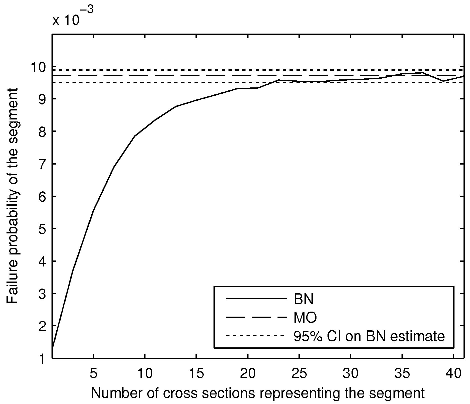
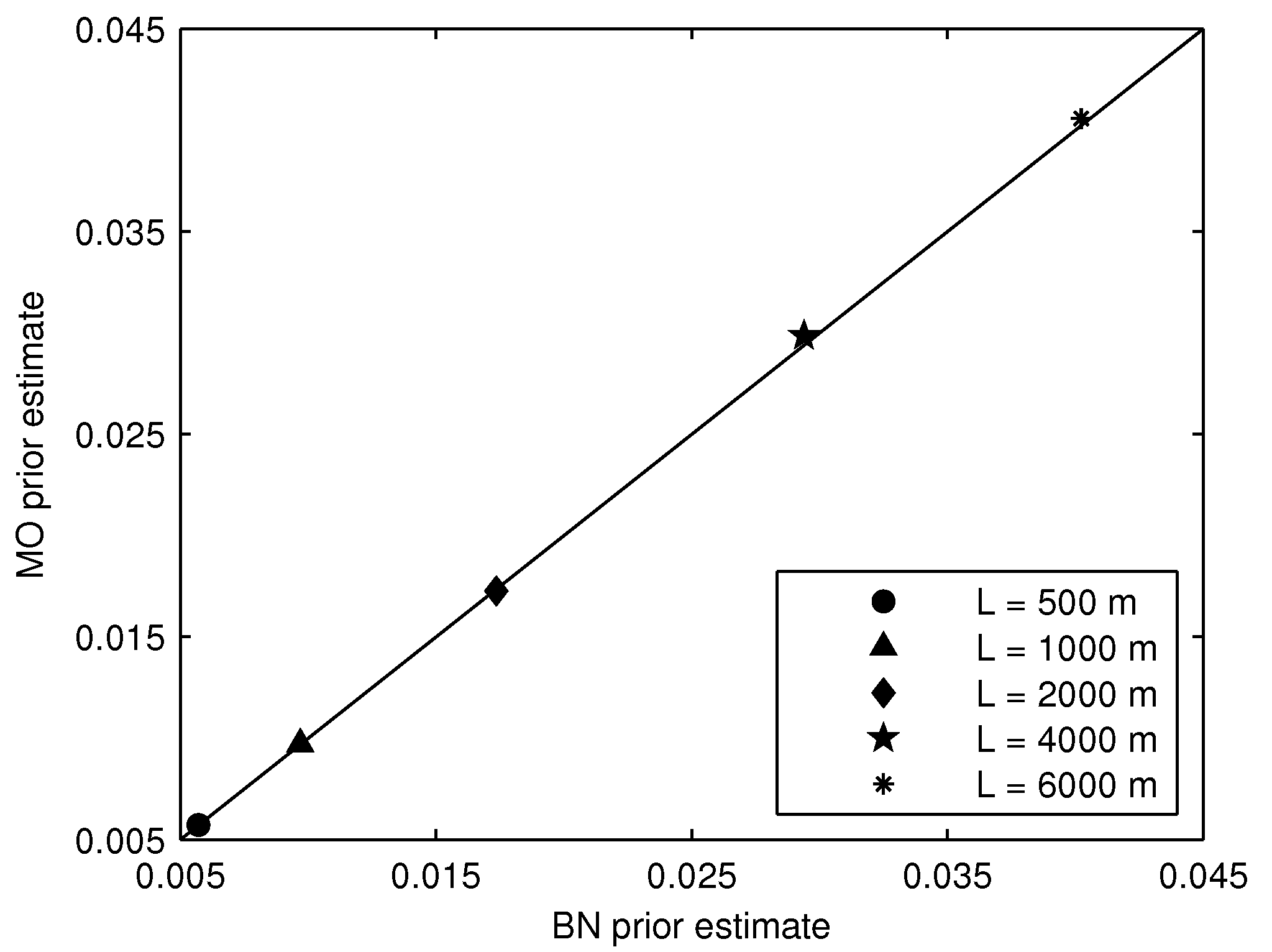
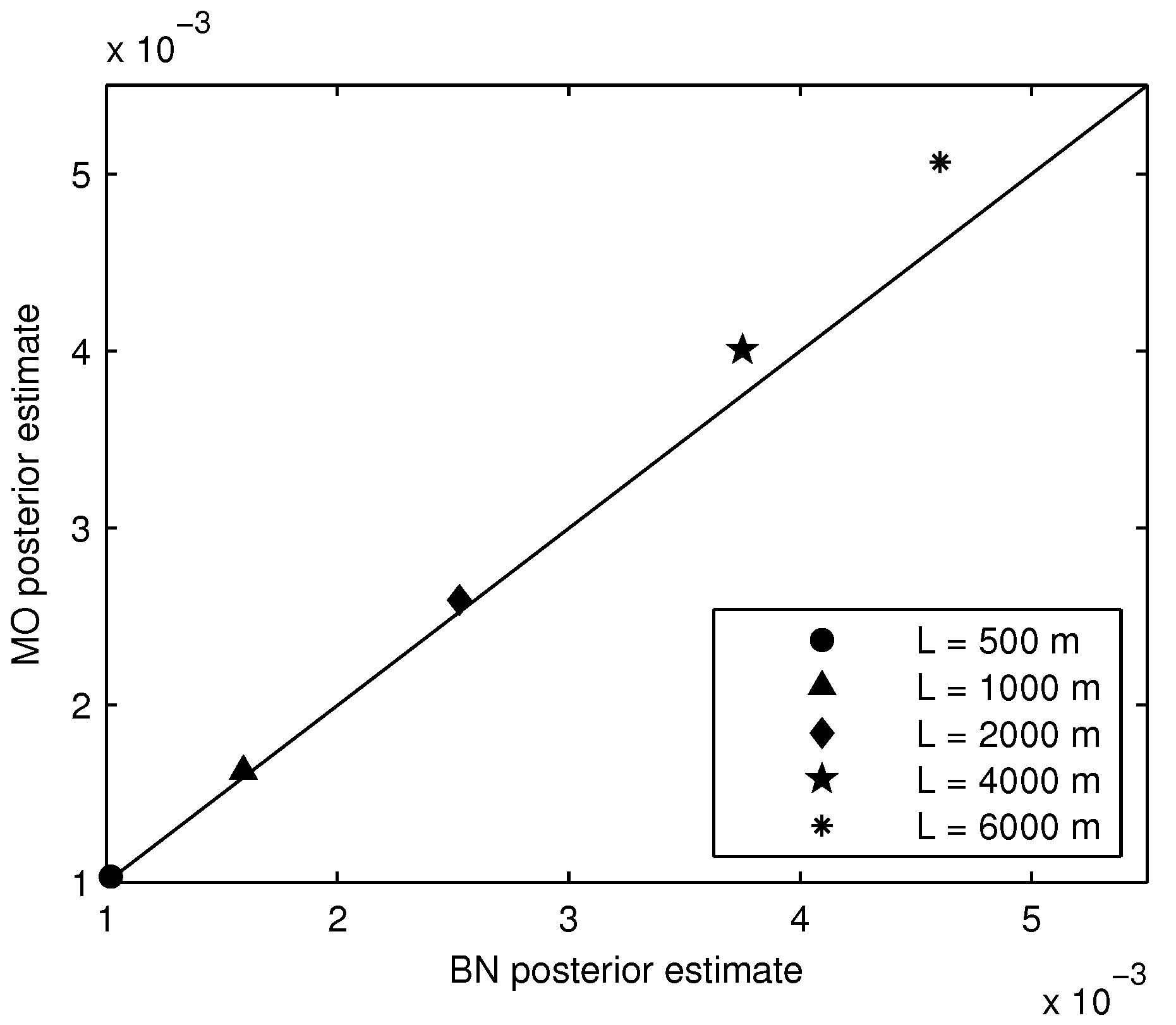
The prior and posterior segment failure probabilities calculated by the two methods are in strong agreement. Slight discrepancies were found for posterior segment failure probabilities for long segments (4000 and 6000 m), but these differences were less than 10%, and in terms of reliability index, less than 1%. These results provide a strong verification of the MO method for prior analysis, which is used in the levee reliability model Hydra-Ring. They also provide an important verification of the MO method for posterior analysis, which has a lot of potential. The speed of the MO method makes it possible to efficiently update failure probabilities of numerous levee segments with abundant survival observations.

Given the strong agreement between BN and MO results, and the relative efficiency of the MO method, we advocate use of the latter in practice. However, we must emphasize that the examples considered in this paper do not represent an exhaustive set of cases. For failure probability updating with survival observations, we advocate comparing the BN and MO output for each new type of application (e.g., new limit state function, new set of variable distribution types or correlation parameters). Once the results are verified, the MO method can be used with confidence for all examples of the same type.

Finally, we strongly advocate the use of either the BN or MO method to account for the length effect in reliability analysis over some of the more simplified approaches found in the literature.

References

1. Bažant, Z.P.; Chen, E.P. Scaling of Structural Failure. Appl. Mech. Rev. 1997, 50, 593–627. [Google Scholar] [CrossRef]
2. Vanmarcke, E.H. On the distribution of the first-passage time for normal stationary random processes. J. Appl. Mech. 1975, 42, 215–220. [Google Scholar] [CrossRef]
3. Vanmarcke, E.H. Random Fields: Analysis and Synthesis, 1st ed.; MIT Press: Cambridge, MA, USA, 1983; 394p. [Google Scholar]
4. Li, Y.; Hicks, M.A. Comparative study of embankment reliability in three dimensions. NUMGE 2014, 1, 467–472. [Google Scholar]
5. Li, Y.; Hicks, M.A. Reliability of earth slopes. ASCE J. Geotech. Eng. Div. 1977, 103, 1247–1265. [Google Scholar]
6. Bowles, D.S.; Chauhan, S.S.; Anderson, L.R.; Grove, R.C. Baseline risk assessment for Herbert Hoover dike. In Proceedings of the ANCOLD Conference on Dams, Perth, Australia, 24–28 October 2012; pp. 1–26. [Google Scholar]
7. U.S. Bureau of Reclamation. Dam Safety Risk Analysis: Best Practices and Risk Methodology Training Manual. 2011. Available online: https://www.usbr.gov/ssle/damsafety/risk/index.html (accessed on 11 December 2019).
8. Steenbergen, H.; Lassing, B.A.; Vrouwenvelder, T.; Waarts, P. Reliability Analysis of Flood Defence Systems. Heron 2004, 49, 51–73. [Google Scholar]
9. Vrouwenvelder, A.C.M.W. Spatial effects in reliability analysis of flood protection systems. In Proceedings of the Second IFED Forum, Lake Louise, AB, Canada, 26–29 April 2006. [Google Scholar]
10. Jongejan, R.; Maaskant, B.; ter Horst, W.; Havinga, F.; Roode, N.; Stefess, H. The VNK2-project: A fully probabilistic risk analysis for all major levee systems in the Netherlands. IAHS Publ. 2013, 357, 75–85. [Google Scholar]
11. Jongejan, R.; Maaskant, B. Quantifying Flood Risks in the Netherlands. Risk Anal. 2015, 35, 252–264. [Google Scholar] [CrossRef]
12. Jongejan, R.; Maaskant, B. Applications of VNK2, a fully probabilistic risk analysis for all major levee systems in The Netherlands. In Proceedings of the FloodRisk, Rotterdam, The Netherlands, 19–23 November 2012. [Google Scholar]
13. Kanning, W. The Weakest Link: Spatial Variability in the Piping Failure Mechanism of Dikes. Ph.D. Thesis, Delft University of Technology, Delft, The Netherlands, 14 December 2012. [Google Scholar]
14. Vrijling, J.K.; Schweckendiek, T.; Kanning, W. Safety Standards of Flood Defenses. In Proceedings of the International Symposium on Geotechnical Safety and Risk, Munich, Germany, 2–3 June 2011. [Google Scholar]
15. Kanning, W.; Schweckendiek, T.; Vrouwenvelder, T.; Calle, E. The Length-Effect in the Reliability of Flood Defenses. 2020; manuscript in preparation. [Google Scholar]
16. Maljaars, J.; Vrouwenvelder, A.C.W.M. Probabilistic fatigue life updating accounting for inspections of multiple critical locations. Int. J. Fatigue 2014, 68, 24–37. [Google Scholar] [CrossRef] [Green Version]
17. Schweckendiek, T.; Vrouwenvelder, A.C.W.M.; Calle, E.O.F. Updating piping reliability with field performance observations. Struct. Saf. 2014, 47, 13–23. [Google Scholar] [CrossRef]
18. Bensi, M.; Der Kiureghian, A.; Straub, D. Bayesian network modeling of correlated random variables drawn from a Gaussian random field. Struct. Saf. 2011, 33, 317–332. [Google Scholar] [CrossRef] [Green Version]
19. Langseth, H.; Nielsen, T.D.; Rumí, R.; Salmerón, A. Inference in hybrid Bayesian networks. RESS 2009, 51, 485–498. [Google Scholar] [CrossRef] [Green Version]
20. Straub, D.; Der Kiureghian, A. Bayesian Network Enhanced with Structural Reliability Methods: Methodology. J. Eng. Mech. 2010, 136, 1248–1258. [Google Scholar] [CrossRef] [Green Version]
21. Neil, M.; Tailor, M.; Marquez, D. Inference in Bayesian networks using dynamic discretisation. Stat. Comput. 2007, 17, 219–233. [Google Scholar] [CrossRef] [Green Version]
22. Kurowicka, D.; Cooke, R.M. Distribution—Free Continuous Bayesian Belief Nets. In Proceedings of the Mathematical Methods in Reliability Conference, Santa Fe, NM, USA, 21–25 June 2004. [Google Scholar]
23. Hanea, A.M.; Kurowicka, D.; Cooke, R.M. Hybrid Method for Quantifying and Analyzing Bayesian Belief Nets. Qual. Reliab. Eng. Int. 2006, 22, 613–729. [Google Scholar] [CrossRef]
24. Hanea, A.M.; Kurowicka, D.; Cooke, R.M.; Ababei, D.A. Mining and visualising ordinal data with non-parametric continuous BBNs. Comput. Stat. Data Anal. 2010, 54, 668–687. [Google Scholar] [CrossRef]
25. Hanea, A.M.; Napoles Morales, O.; Ababei, D.A. Non-parametric Bayesian networks: Improving theory and reviewing applications. RESS 2015, 144, 265–284. [Google Scholar] [CrossRef]
26. Sklar, A. Fonctions de réparation à n dimensions et leurs marges. Publ. Inst. Statist. Univ. Paris 1959, 8, 229–231. [Google Scholar]
27. Lebrun, R.; Dutfoy, A. An innovating analysis of the Nataf transformation from the copula viewpoint. Probab. Eng. Mech. 2009, 24, 312–320. [Google Scholar] [CrossRef]
28. Diermanse, F.L.M.; Geerse, C.P.M. Correlation models in flood risk analysis. RESS 2012, 105, 64–72. [Google Scholar] [CrossRef]
29. Lebrun, R.; Dutfoy, A. Do Rosenblatt and Nataf isoprobabilistic transformations really differ? Probab. Eng. Mech. 2009, 24, 577–584. [Google Scholar] [CrossRef]
30. Hanea, A.M. Algorithms for Non-Parametric Bayesian Belief Nets. Ph.D. Thesis, Delft University of Technology, Delft, The Netherlands, 15 December 2008. [Google Scholar]
31. Morales-Napoles, O.; Worm, D.; Dillingh, B. Framework for Probabilistic Scale Transition in Physico-Chemical Modeling of Asphalt; TNO Report Project Number 034.24789; TNO: Delft, The Netherlands, 2011. [Google Scholar]
32. Weber, R.O.; Talkner, P. Some remarks on spatial correlation function models. Mon. Weather Rev. 1993, 121, 2611–2617. [Google Scholar] [CrossRef]
33. Eaton, M.L. Multivariate Statistics: A Vector Space Approach; Institute for Mathematical Sciences: Beachwood, OH, USA, 2007. [Google Scholar]
34. Smith, A.F.M.; Gelfand, A.E. Bayesian statistics without tears: A sampling–resampling perspective. Am. Stat. 1992, 46, 84–88. [Google Scholar]
35. Gilks, W.R. Markov Chain Monte Carlo; Wiley Online Library: Hoboken, NJ, USA, 2005. [Google Scholar]
36. Melchers, R.E. Safety and risk in structural engineering. Progr. Struct. Eng. Mater. 2002, 4, 193–202. [Google Scholar] [CrossRef]
37. Vanmarcke, E. Random Fields: Analysis and Synthesis, Revised and Expanded New Ed.; World Scientific: Singapore, 2010. [Google Scholar]
Figure 1. Spatial scales: A levee segment and a cross section.
Safety 06 00007 g001
Figure 2. Random field perspective rather than a point estimate considered in a failure model.
Safety 06 00007 g002
Figure 3. Spatial variability of the limit state function Z for a strongly autocorrelated Z function (top) and a weakly autocorrelated Z function (bottom).
Safety 06 00007 g003
Figure 4. Example three-variable Bayesian network, where X 1 and X 2 are the independent parents of X 3 .
Safety 06 00007 g004
Figure 5. Example of a Bayesian Network (BN) for cross sectional levee failure probability with three resistance variables R 1 , R 2 , and R 3 , and a load variable S.
Safety 06 00007 g005
Figure 6. Example of a levee segment whose spatial variability is represented by three cross sections.
Safety 06 00007 g006
Figure 7. BN for a levee segment, in this example represented by three cross sections, each with autocorrelated resistance variables R 1 , R 2 , and R 3 , and one common load variable S.
Safety 06 00007 g007
Figure 8. BN representing the limit state function Z = R 1 + R 2 - S for one cross section.
Safety 06 00007 g008
Figure 9. Posterior constraints on R 1 and R 2 , imposed by the observation that Z > 0 for an observed value of S, S o b s = 8 .
Safety 06 00007 g009
Figure 10. BN for a segment, shown here for three cross sections, where cross-sectional failure is defined by the limit state function in Equation (11).
Safety 06 00007 g010
Figure 11. Prior densities of R ( R = R 1 + R 2 ) and S, and the observed load s o b s = 4 . 38 corresponding to the 99% quantile of S ( P ( S < s o b s ) = 0 . 99 ).
Safety 06 00007 g011
Figure 12. Comparison of the BN with the modified outcrossing (MO) estimate, for Z = R 1 + R 2 - S , with R 1 and R 2 lognormally distributed, and S Gumbel-distributed, prior to incorporating a survival observation.
Safety 06 00007 g012
Figure 13. Comparison of BN and MO segment failure probability estimates (shown together with the 1:1 line, which represents perfect agreement).
Safety 06 00007 g013
Figure 14. Comparison of posterior segment failure probability estimates computed with the BN and MO methods; 95% confidence intervals on the BN estimate are also indicated.
Safety 06 00007 g014
Figure 15. Comparison of BN and MO posterior segment failure probability estimates (shown together with the 1:1 line, which represents perfect agreement).
Safety 06 00007 g015