SOM is applied in SKM to coded data obtained from an occupational accident database. SOM can represent the occupational data set in a two-dimension map. This process reflects the data similarity within occupational databases: Accidents with similar descriptive parameters are projected into the next units and very different accidents are projected into distant units.
2.1.1. Pre-Processing Phase
The data set used in this study was taken from the INAIL (Italian institution for insurance against accidents at work) database, where accidents are reported according to the ESAW taxonomy.
Each accident is described by more than 20 variables, that is: Geographical location of the accident, time of occurrence, details about the injured party (activity, age …), dynamics of the accident (deviation from normal procedures, contact and mode of injury) and circumstances of the accident (workstation, working environment).
The combination of the number of elements and the huge number of descriptive variables requires a great calculation effort. Furthermore, most of the variables are categorical elements, whereas the algorithms for SOM and K-Means calculation require numerical ones.
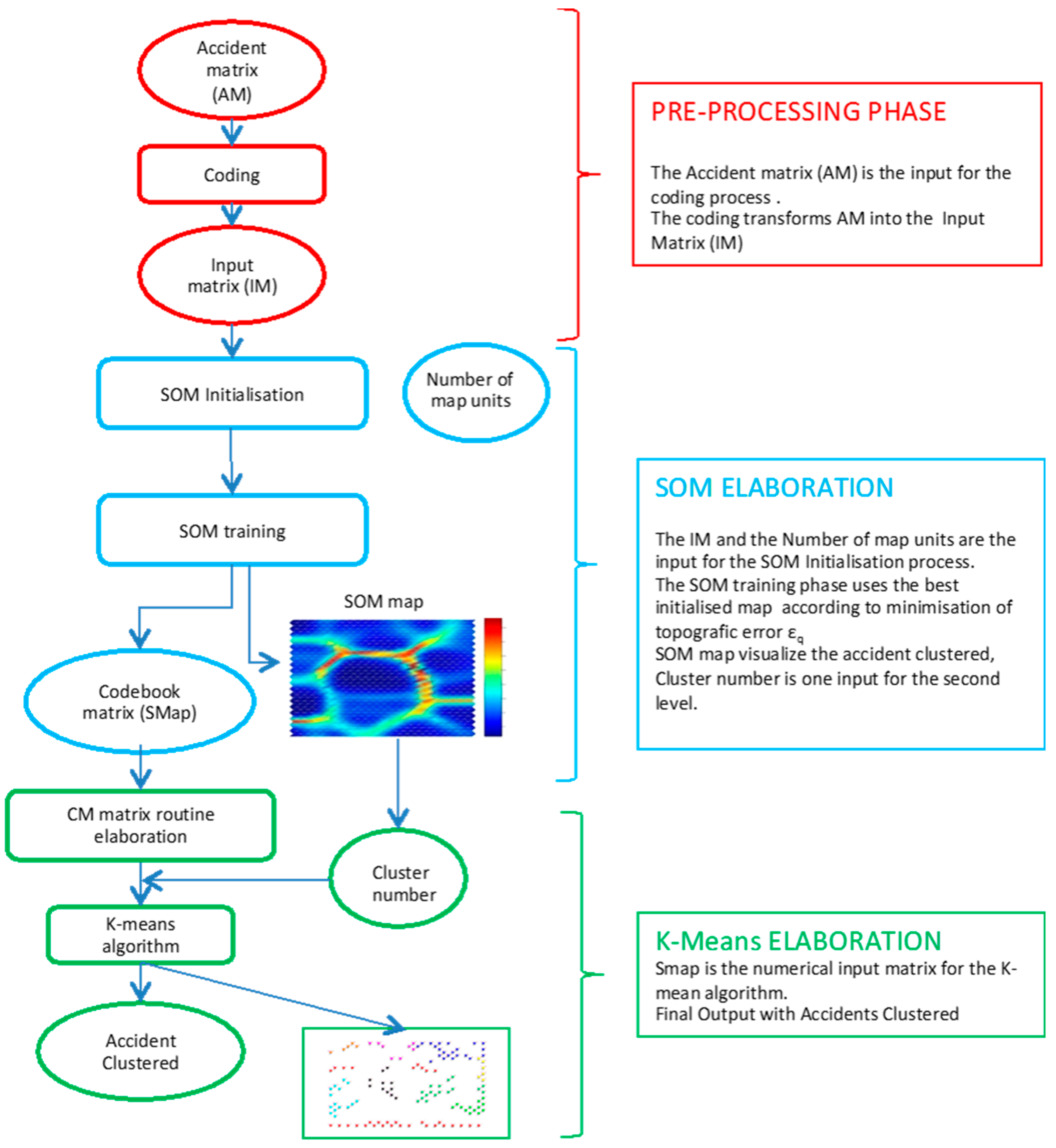
The method requires a pre-processing phase to adapt the data from the occupational accident database to the algorithm characteristic. The pre-processing phase overcomes these two drawbacks by means of a two-step coding procedure.
The first step is focused on the construction of an Accident Matrix (AM). The AM contains the occupational accidents that have to be processed; this matrix has a dimension D, which is obtained from:
where n is the accident number, and m is the number of variables selected from among those available in the ESAW classification to describe each accident.
Each variable can assume different values but, to limit the computational efforts, these values are limited with respect to the hierarchical structure of the ESAW classification.
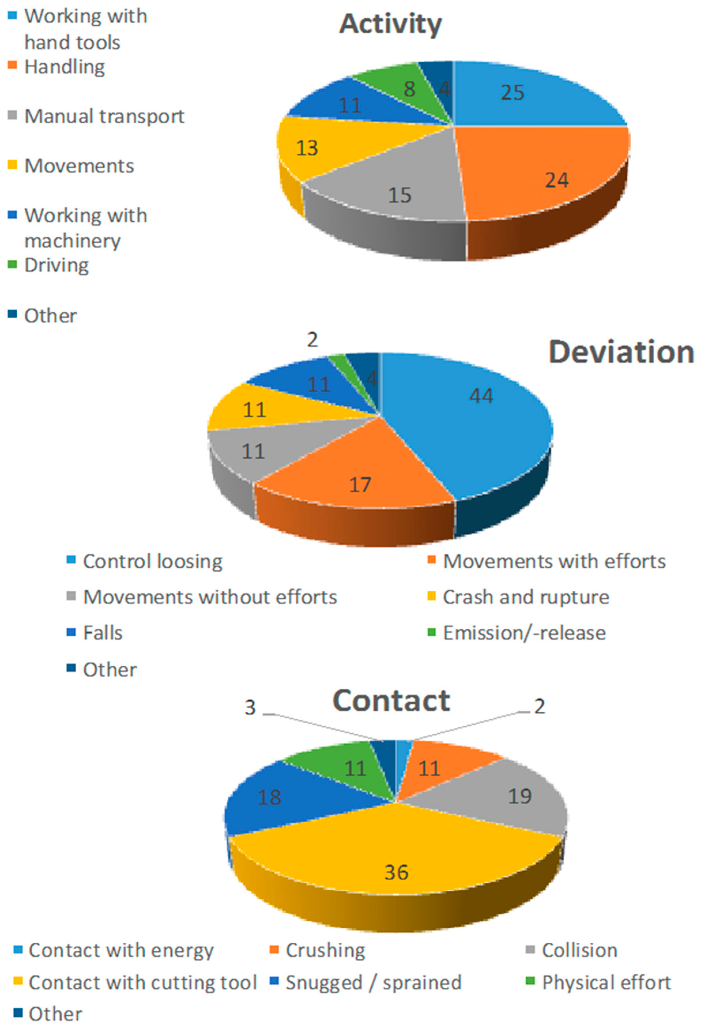
Table 1 shows part of the ESAW taxonomy for the “Activity” variable: According to the coding procedure, the labels from 41 to 49, pertaining to “handling of objects”, will be replaced by the upper level label 40, while the labels from 61 to 69, pertaining to “movement”, will be replaced by label 60.
The second step involves numerical coding; each accident is coded from a sequence of categorical information to a sequence of numbers.
As reported in Palamara et al. [
6], each parameter is coded in a numerical vector that contains a sequence of zeros and a single 1. The union of the vectors that describe the variables used for the analysis leads to the complete coding of each accident.
The resulting vector will have as many 1s as the variables and as many 0s as the total number of categories for all the variables, less the number of variables.
The “Input matrix” (IM) contains all the accidents coded into numerical vectors; its dimension (D
input) is obtained from:
where n is the number of accidents and p is obtained from the number of variables multiplied by the number of categories used to describe them.
Let us assume that an accident is described by 4 variables and each variable can have 5 possible different categories. The parameter p will thus have a value of 20.
This coding procedure is run automatically through the use of conversion tables that allow an univocal correspondence between categorical values and numerical vectors to be achieved, as shown in
Table 2.
At the end of the pre-processing phase, the AM that originally contained a group of selected occupational accidents is coded into the IM that contains an equivalent number of numerical vectors.
2.1.2. SOM Elaboration
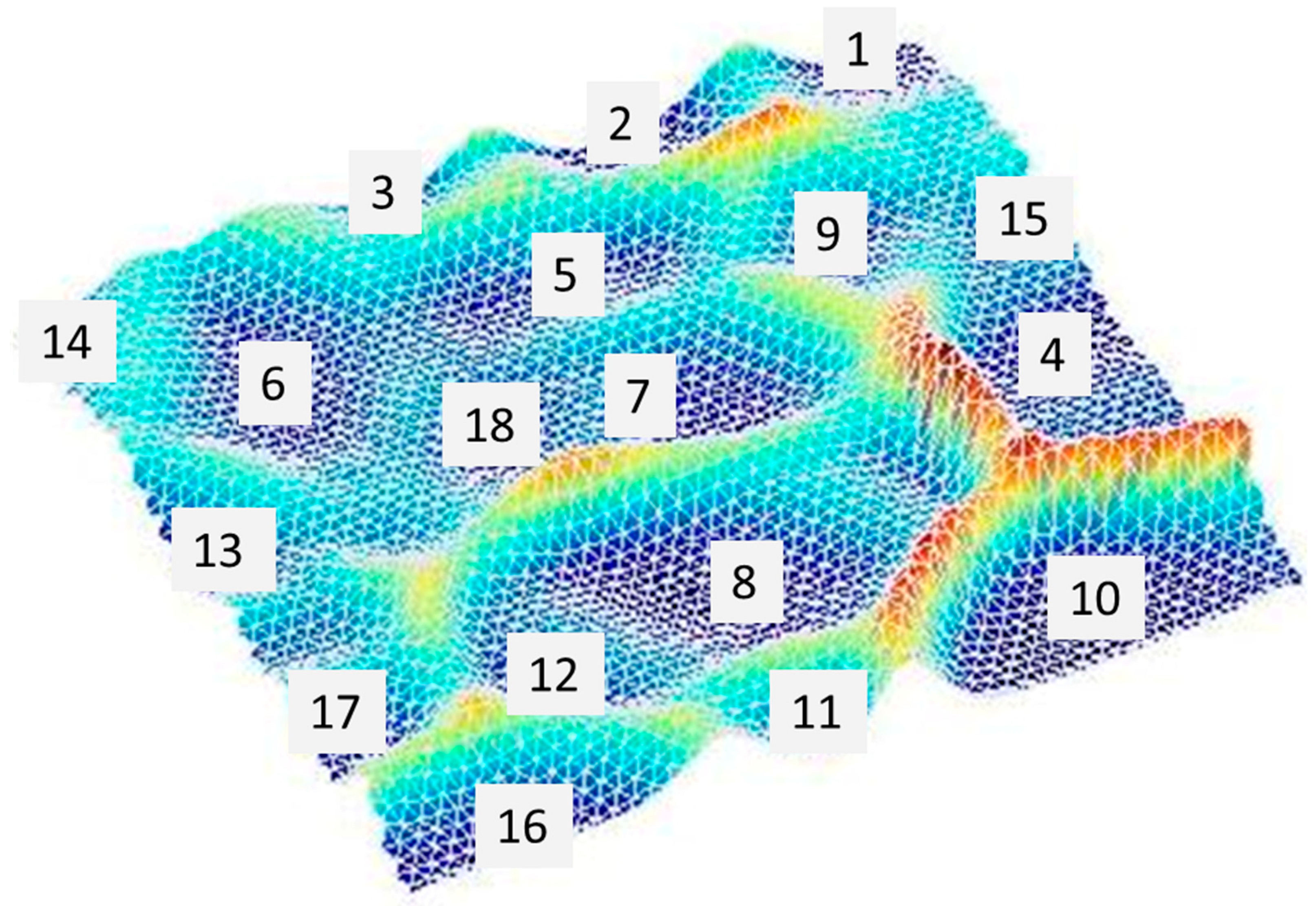
With reference to
Figure 1, the first level of SKM contains the Self Organizing Map (SOM) algorithm, which allows multidimensional vectors to be represented in a two-dimensional space, while preserving the topology of the multidimensional space.
SOM is based on a neural network scheme that is formed by two layers: The first layer is made up of the input vectors; the second layer is a map that is characterized by several units that are set by the user.
There are several ways of calculating SOM; SKM is configured with the “batch SOM” approach [
27], which guarantees faster and more efficient performances for complex data sets than the traditional approach.
This approach uses an iterative calculation of matrices and it depends on the initial condition, as will be discussed later on.
The input data are fed as a single block, that is, “batch” [
27], and the algorithm assigns a random vector of equal size as the input data, called “weight”, to each unit during the initialization phase.
In the training phase, the algorithm calculates the Hamming distance [
28] between IM elements and all the unit weights.
This is an iterative process in which, at each iteration, the input data set is presented as a batch to the SOM, and the algorithm calculates the distance between each input vector and each unit weight vector. As in a competitive learning algorithm, the units in the map layer compete to represent the input data and, for each input data, the unit whose weight vector is closest to it wins the competition. This unit is called the ‘Best Matching Unit’ (BMU).
The weight vector values of the winning units are updated, at each iteration, in order to make each output unit representative of a particular kind of input [
29], together with those of the surrounding units. The magnitude of this update depends on the distance between the winning unit in the network and the other units, according to the Gaussian neighborhood function.
The value of the neighborhood function decrees with the distance from the winning unit. In this way, the weight of the units around the winner is modified, while it remains almost unaltered for distant units.
This ensures that the data projected into the next units are similar.
The process ends when each input data is coupled with a BMU.
As mentioned above, this iterative process depends on the initial condition; in order to deal with this dependency, the SKM allows several independent initializations, named seeds, to be made, and these produce several different rough maps.
SKM evaluates, for each map, the topology preservation accuracy that describes how well the data, which are close in the input space, are projected to close units in the SOM.
The topology preservation accuracy is pointed out by the topographic error, which is given by the following equation:
where
N is the data number,
xi is the
ith input data and
u(
xi) is equal to 1, if the first and the second best matching units are not adjacent units, otherwise it is zero.
The topographic error minimization leads to the identification of the best map among all those generated.
At the end of the training process, the map has organized itself by mapping input data into SOM units and, in particular, by connecting similar input data to neighboring units.
The number of units has to be chosen by the user. There is not an objective criterion to set it up and, as discussed in Comberti et al. [
7], a rule of thumb is to set it with a lower value than the number of analysed occupational accidents.
The output of the training process is a bi-dimensional map and a numerical output that is represented by a matrix called SMap.
SMap contains the numerical code of the map and the dimension of this matrix, which is obtained from:
where U is the number of the unit of the map and p is the same as for Equation (2).
Each element is characterized by a sequence of real numbers that represent the weights of each unit, which is also called prototype vector [
15]. The weights are basically proportional to the number and type of data that are projected into the corresponding unit, consequently, all the units without projected data are characterized by a similar prototype vector.
SKM defines a new matrix, called Clustering Matrix (CM), from SMap.
CM contains a number of elements that is equal to the number of IM elements, and the prototype vector of the corresponding activated unit defines each element.
The CM matrix and the Cluster number, evaluated from the SOM map interpretation, are the input data for the second level of the method.
2.1.3. K-Means Elaboration
As mentioned in the introduction, the second level of clustering is based on a K-Means algorithm.
K-Means is based on the concept of cluster centers, which are called ‘centroids’. A centroid is a point in the data space that represents a cluster. The algorithm finds the positions of the cluster centroids in the input space, and minimizes an objective function E, the ‘square-error distortion’.
After each data has been assigned, the centroid of each cluster has clearly changed, on the basis of the positions of the data in the space and on the random initial position of the centroid.
Therefore, a new cluster centroid is calculated in such a way that the sum of the squared distances is minimized.
The process continues with the calculation of the new distances between each input data and each centroid and re-assigning the data to the nearest centroid. This process is repeated until no more changes occur. In other words, the algorithm ends when all the data have been assigned to their nearest centroids.
The K-Means algorithm requires three user-specified parameters: A number of clusters K, cluster initialization and a distance metric.
The most critical choice is
K. Although no perfect mathematical criterion exists, several heuristics criteria [
30] are available to choose
K.
The value of K in SKM is obtained from a SOM map visual evaluation. The CM matrix constitutes the input data for the K-Means algorithm.
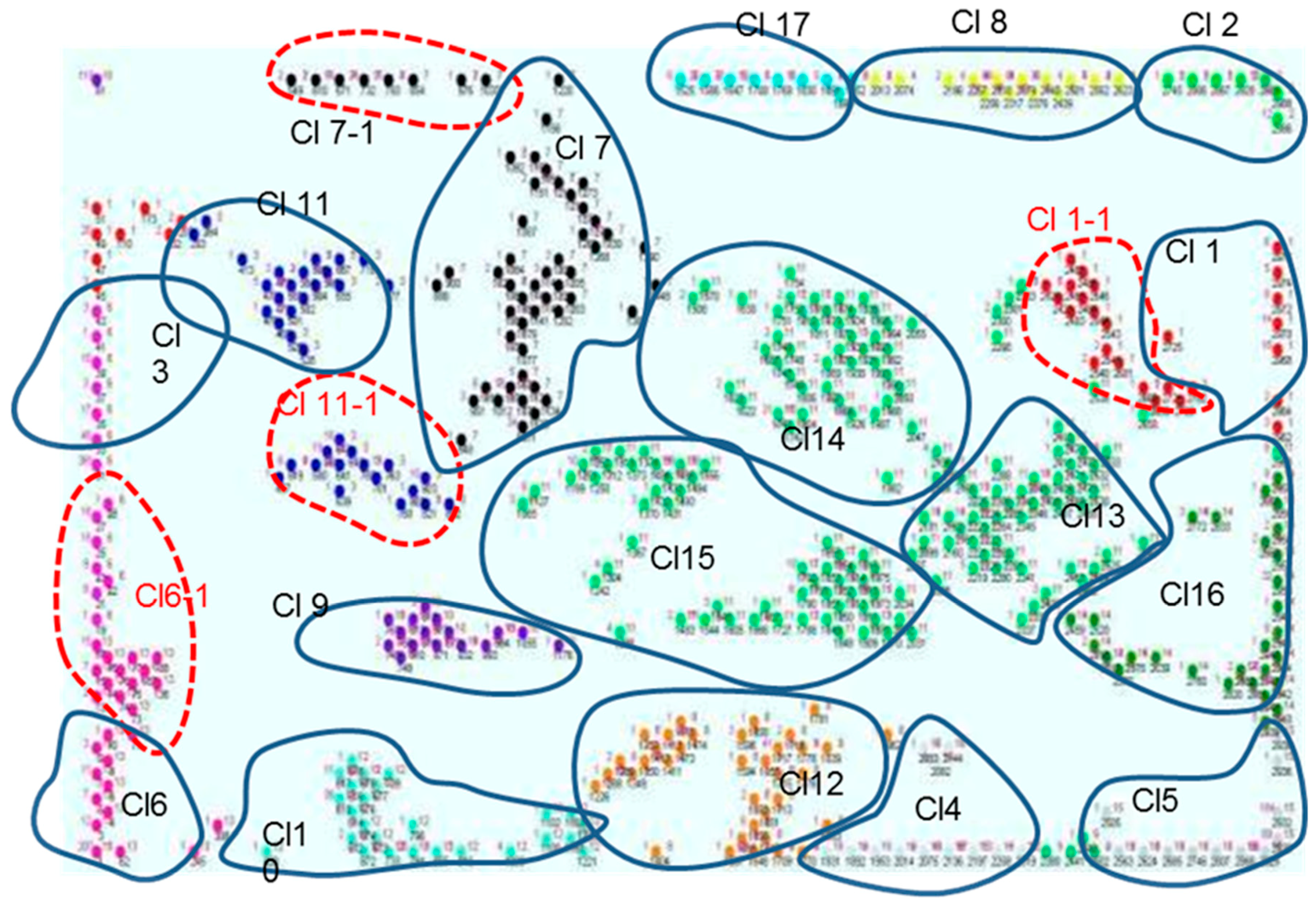
The clustering phase provides a data partition that is summarized in a chart, where each occupational accident is attributed to a specific cluster, and a graphical output, dedicated to clustering visualization, is drawn, as shown in
Figure 2.
The graph shows the distribution of activated units in the SOM map domain. Each unit is described by different colors, depending on the membership cluster. Each unit is marked by its own number (see the green circle in
Figure 2), the number of projected elements (blue circle), and the cluster to which the unit belongs (red circle).
This graphical elaboration makes the comparison between several partitions easier, thus the evaluation of clustering accuracy becomes more immediate and intuitive.
With this visualization, it is also possible to carry out a comparison with the corresponding SOM map.

 ,
, 