

Limitations of Out-of-Distribution Detection in 3D Medical Image Segmentation


Abstract
:1. Introduction
- We demonstrate the severe limitations of the existing OOD detection methods with 3D medical images;
- We designed and now release the corresponding benchmark that can be used as a starting point for related research;
- We propose a method, IHF, and suggest it as a solid baseline for OOD detection with 3D medical images.
2. Data
- We included two large publicly available CT and MRI in-distribution (ID) datasets to cover the most frequent volumetric modalities.
- We ensured both datasets had a downstream segmentation task, allowing us to use the full spectrum of methods.
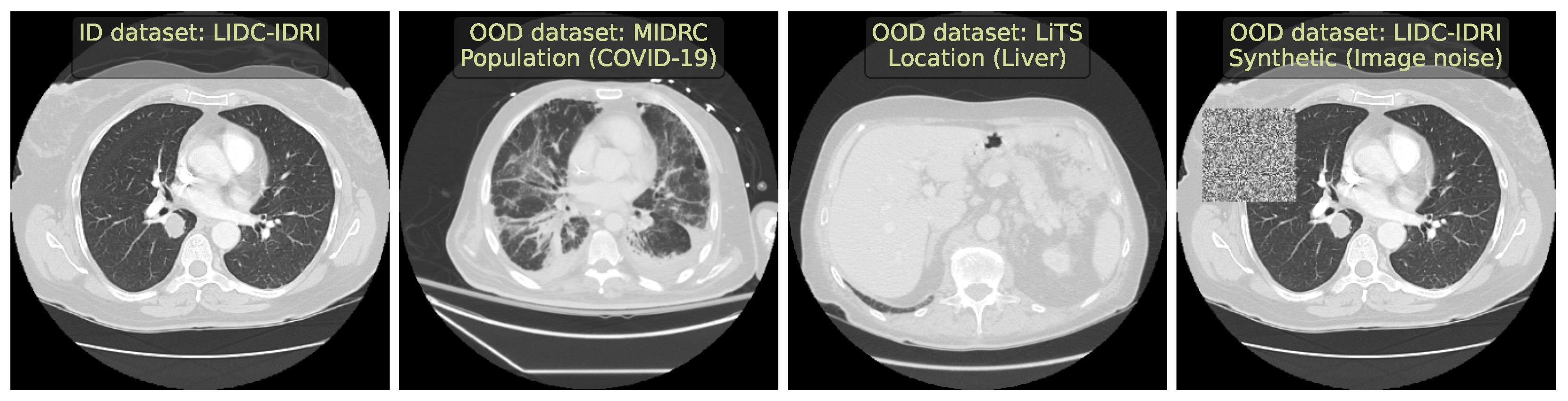
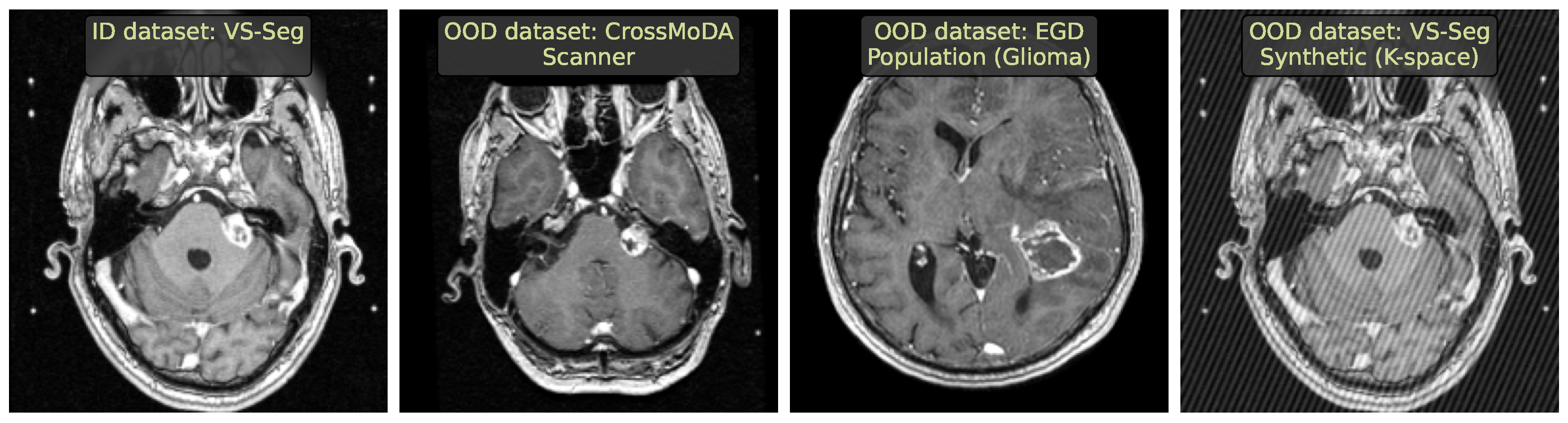
- We selected diverse OOD datasets that simulated the clinically occurring sources of anomalies: changes in acquisition protocol, patient population, or anatomical region. All these datasets are publicly available.
2.1. Lung Nodules Segmentation
2.2. Vestibular Schwannoma Segmentation
2.3. Problem Setting
3. Methods
3.1. Methods Selection
3.2. Method Implementation
3.2.1. Entropy
3.2.2. Ensemble
3.2.3. MCD
3.2.4. SVD
3.2.5. G-ODIN
3.2.6. MOOD-1
3.2.7. Volume Predictor
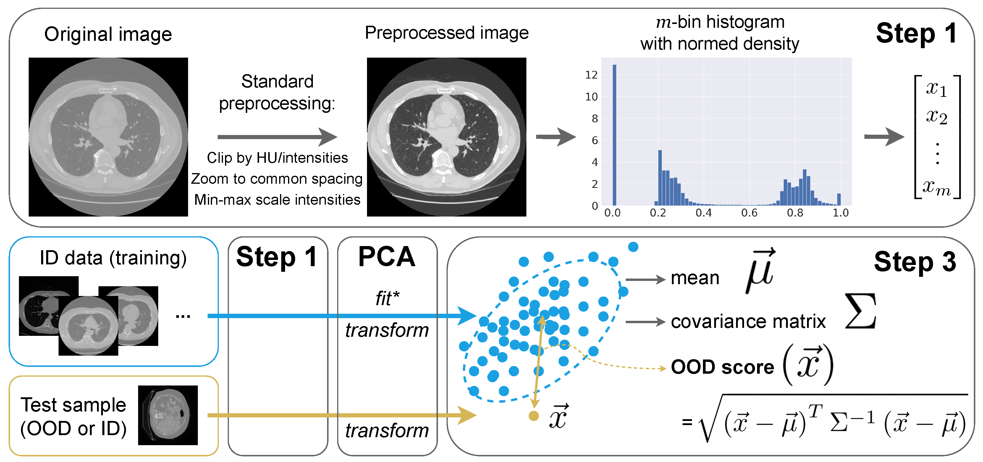
3.3. Intensity Histogram Features
- Step 1: Preprocessing and histograms
- We interpolate images to the median ID spacing. So, in all CT and MRI experiments, we use mm.
- We clip image intensities to Hounsfield units for CT (a standard lung window) and [1th percentile, 99th percentile] for MRI.
- We MinMax-scale image intensities to the range.
- Step 2: Principal Component Analysis (PCA)
- Step 3: OOD detection algorithm
4. Experimental Setup
4.1. Downstream Task
4.1.1. Data Preprocessing
4.1.2. Architecture and Training
4.1.3. Segmentation Evaluation
4.2. OOD Detection Evaluation
5. Results
5.1. Benchmarking
5.2. In-Depth Benchmark Analysis
- OOD methods should be studied under a benchmark with diverse OOD challenges.
- Setups should represent clinically occurring cases.
- Potential biases in the benchmark should be explored using simple methods, such as IHF or Volume predictor.
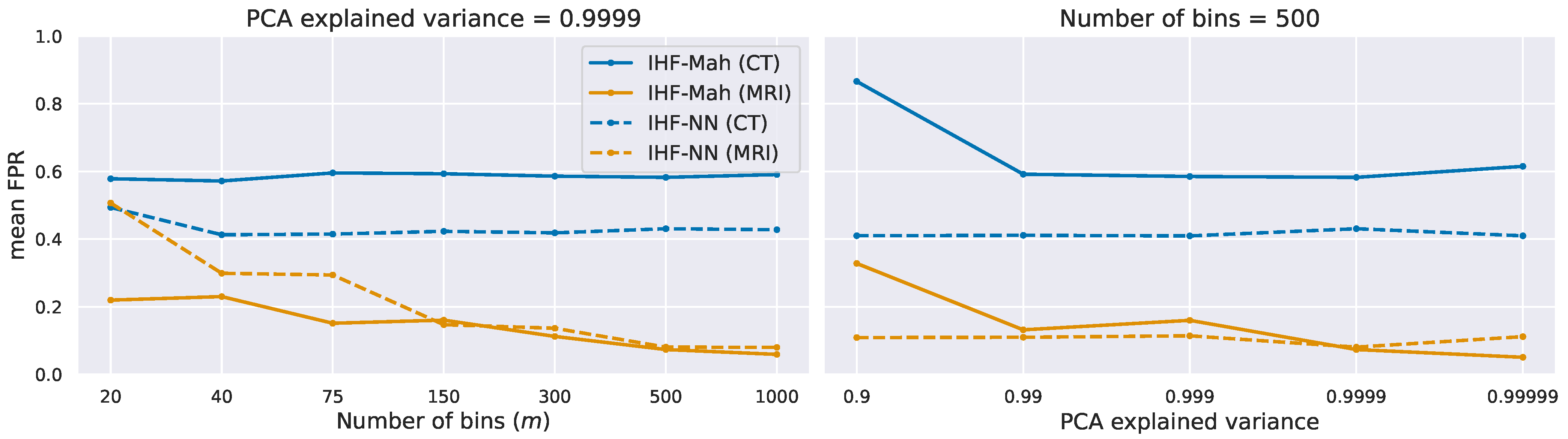
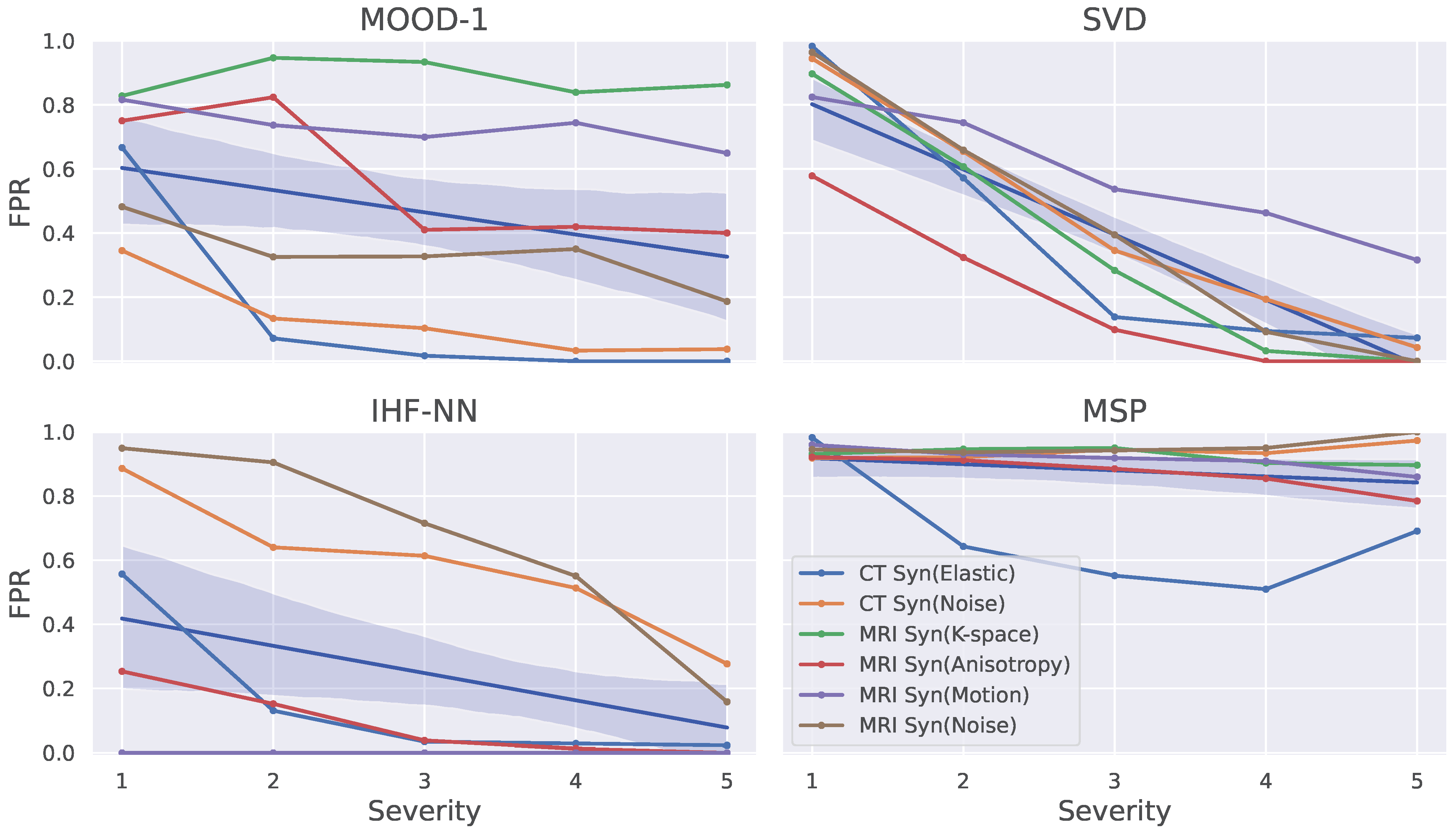
5.3. Ablation Study on Synthetic Data
6. Discussion
6.1. Benchmark Design
6.2. Uncertainty Estimation
6.3. Other IHF Applications
7. Conclusions
Author Contributions
Funding
Institutional Review Board Statement
Informed Consent Statement
Data Availability Statement
Acknowledgments
Conflicts of Interest
Abbreviations
| AD | Anomaly detection |
| AUROC | Area under receiver operating characteristic |
| COVID-19 | Coronavirus disease 19 |
| CT | Computed Tomography |
| DL | Deep Learning |
| DSC | Dice similarity coefficient |
| FPR | False positive rate |
| ID | In-distribution |
| IHF | Intensity Histogram Features |
| MCD | Monte Carlo dropout |
| MDPI | Multidisciplinary Digital Publishing Institute |
| MOOD | Medical out-of-distribution |
| MRI | Magnetic resonance imaging |
| OOD | Out-of-distribution |
| PCA | Principal Component Analysis |
| SVD | Singular value decomposition |
| TPR | True positive rate |
| UE | Uncertainty estimation |
References
- Wang, M.; Deng, W. Deep Visual Domain Adaptation: A Survey. Neurocomputing 2018, 312, 135–153. [Google Scholar] [CrossRef]
- Kompa, B.; Snoek, J.; Beam, A.L. Second opinion needed: Communicating uncertainty in medical machine learning. NPJ Digit. Med. 2021, 4, 4. [Google Scholar] [CrossRef] [PubMed]
- Yang, J.; Zhou, K.; Li, Y.; Liu, Z. Generalized out-of-distribution detection: A survey. arXiv 2021, arXiv:2110.11334. [Google Scholar]
- Hendrycks, D.; Gimpel, K. A baseline for detecting misclassified and out-of-distribution examples in neural networks. arXiv 2016, arXiv:1610.02136. [Google Scholar]
- Hendrycks, D.; Basart, S.; Mazeika, M.; Mostajabi, M.; Steinhardt, J.; Song, D. Scaling out-of-distribution detection for real-world settings. arXiv 2019, arXiv:1911.11132. [Google Scholar]
- Mahmood, A.; Oliva, J.; Styner, M. Multiscale score matching for out-of-distribution detection. arXiv 2020, arXiv:2010.13132. [Google Scholar]
- Pacheco, A.G.; Sastry, C.S.; Trappenberg, T.; Oore, S.; Krohling, R.A. On out-of-distribution detection algorithms with deep neural skin cancer classifiers. In Proceedings of the IEEE/CVF Conference on Computer Vision and Pattern Recognition Workshops, Seattle, WA, USA, 14–19 June 2020; pp. 732–733. [Google Scholar]
- Berger, C.; Paschali, M.; Glocker, B.; Kamnitsas, K. Confidence-based out-of-distribution detection: A comparative study and analysis. In Uncertainty for Safe Utilization of Machine Learning in Medical Imaging, and Perinatal Imaging, Placental and Preterm Image Analysis; Springer: Berlin/Heidelberg, Germany, 2021; pp. 122–132. [Google Scholar]
- Cao, T.; Huang, C.W.; Hui, D.Y.T.; Cohen, J.P. A benchmark of medical out of distribution detection. arXiv 2020, arXiv:2007.04250. [Google Scholar]
- Litjens, G.; Kooi, T.; Bejnordi, B.E.; Setio, A.A.A.; Ciompi, F.; Ghafoorian, M.; Van Der Laak, J.A.; Van Ginneken, B.; Sánchez, C.I. A survey on deep learning in medical image analysis. Med. Image Anal. 2017, 42, 60–88. [Google Scholar] [CrossRef]
- Karimi, D.; Gholipour, A. Improving Calibration and Out-of-Distribution Detection in Deep Models for Medical Image Segmentation. IEEE Trans. Artif. Intell. 2022, 4, 383–397. [Google Scholar] [CrossRef]
- Zimmerer, D.; Petersen, J.; Köhler, G.; Jäger, P.; Full, P.; Maier-Hein, K.; Roß, T.; Adler, T.; Reinke, A.; Maier-Hein, L. Medical Out-of-Distribution Analysis Challenge 2022. In Proceedings of the 25th International Conference on Medical Image Computing and Computer Assisted Intervention (MICCAI 2022), Singapore, 18–22 September 2022. [Google Scholar] [CrossRef]
- Lambert, B.; Forbes, F.; Doyle, S.; Tucholka, A.; Dojat, M. Improving Uncertainty-based Out-of-Distribution Detection for Medical Image Segmentation. arXiv 2022, arXiv:2211.05421. [Google Scholar]
- Armato III, S.G.; McLennan, G.; Bidaut, L.; McNitt-Gray, M.F.; Meyer, C.R.; Reeves, A.P.; Zhao, B.; Aberle, D.R.; Henschke, C.I.; Hoffman, E.A.; et al. The lung image database consortium (LIDC) and image database resource initiative (IDRI): A completed reference database of lung nodules on CT scans. Med. Phys. 2011, 38, 915–931. [Google Scholar] [CrossRef] [PubMed]
- Morozov, S.; Gombolevskiy, V.; Elizarov, A.; Gusev, M.; Novik, V.; Prokudaylo, S.; Bardin, A.; Popov, E.; Ledikhova, N.; Chernina, V.; et al. A simplified cluster model and a tool adapted for collaborative labeling of lung cancer CT scans. Comput. Methods Programs Biomed. 2021, 206, 106111. [Google Scholar] [CrossRef] [PubMed]
- Tsai, E.B.; Simpson, S.; Lungren, M.P.; Hershman, M.; Roshkovan, L.; Colak, E.; Erickson, B.J.; Shih, G.; Stein, A.; Kalpathy-Cramer, J.; et al. The RSNA International COVID-19 Open Radiology Database (RICORD). Radiology 2021, 299, E204–E213. [Google Scholar] [CrossRef] [PubMed]
- Bilic, P.; Christ, P.F.; Vorontsov, E.; Chlebus, G.; Chen, H.; Dou, Q.; Fu, C.W.; Han, X.; Heng, P.A.; Hesser, J.; et al. The liver tumor segmentation benchmark (lits). arXiv 2019, arXiv:1901.04056. [Google Scholar] [CrossRef]
- Hssayeni, M.; Croock, M.; Salman, A.; Al-khafaji, H.; Yahya, Z.; Ghoraani, B. Computed tomography images for intracranial hemorrhage detection and segmentation. Intracranial Hemorrhage Segm. Using A Deep. Convolutional Model Data 2020, 5, 14. [Google Scholar]
- Shapey, J.; Kujawa, A.; Dorent, R.; Wang, G.; Dimitriadis, A.; Grishchuk, D.; Paddick, I.; Kitchen, N.; Bradford, R.; Saeed, S.R.; et al. Segmentation of vestibular schwannoma from MRI, an open annotated dataset and baseline algorithm. Sci. Data 2021, 8, 1–6. [Google Scholar] [CrossRef]
- Dorent, R.; Kujawa, A.; Cornelissen, S.; Langenhuizen, P.; Shapey, J.; Vercauteren, T. Cross-Modality Domain Adaptation Challenge 2022 (CrossMoDA). 2022. Available online: https://zenodo.org/record/6504722 (accessed on 6 August 2023).
- van der Voort, S.R.; Incekara, F.; Wijnenga, M.M.; Kapsas, G.; Gahrmann, R.; Schouten, J.W.; Dubbink, H.J.; Vincent, A.J.; van den Bent, M.J.; French, P.J.; et al. The Erasmus Glioma Database (EGD): Structural MRI scans, WHO 2016 subtypes, and segmentations of 774 patients with glioma. Data Brief 2021, 37, 107191. [Google Scholar] [CrossRef]
- Souza, R.; Lucena, O.; Garrafa, J.; Gobbi, D.; Saluzzi, M.; Appenzeller, S.; Rittner, L.; Frayne, R.; Lotufo, R. An open, multi-vendor, multi-field-strength brain MR dataset and analysis of publicly available skull stripping methods agreement. NeuroImage 2018, 170, 482–494. [Google Scholar] [CrossRef]
- Pérez-García, F.; Sparks, R.; Ourselin, S. TorchIO: A Python library for efficient loading, preprocessing, augmentation and patch-based sampling of medical images in deep learning. Comput. Methods Programs Biomed. 2021, 208, 106236. [Google Scholar] [CrossRef]
- Yang, J.; Wang, P.; Zou, D.; Zhou, Z.; Ding, K.; Peng, W.; Wang, H.; Chen, G.; Li, B.; Sun, Y.; et al. OpenOOD: Benchmarking Generalized Out-of-Distribution Detection. arXiv 2022, arXiv:2210.07242. [Google Scholar]
- Jungo, A.; Reyes, M. Assessing reliability and challenges of uncertainty estimations for medical image segmentation. In Proceedings of the International Conference on Medical Image Computing and Computer-Assisted Intervention; Springer: Berlin/Heidelberg, Germany, 2019; pp. 48–56. [Google Scholar]
- Zimmerer, D.; Full, P.M.; Isensee, F.; Jäger, P.; Adler, T.; Petersen, J.; Köhler, G.; Ross, T.; Reinke, A.; Kascenas, A.; et al. MOOD 2020: A public Benchmark for Out-of-Distribution Detection and Localization on medical Images. IEEE Trans. Med. Imaging 2022, 41, 2728–2738. [Google Scholar] [CrossRef] [PubMed]
- Mehrtash, A.; Wells, W.M.; Tempany, C.M.; Abolmaesumi, P.; Kapur, T. Confidence Calibration and Predictive Uncertainty Estimation for Deep Medical Image Segmentation. IEEE Trans. Med. Imaging 2020, 39, 3868–3878. [Google Scholar] [CrossRef]
- Smith, L.; Gal, Y. Understanding Measures of Uncertainty for Adversarial Example Detection. arXiv 2018, arXiv:1803.08533. [Google Scholar]
- Lakshminarayanan, B.; Pritzel, A.; Blundell, C. Simple and scalable predictive uncertainty estimation using deep ensembles. Adv. Neural Inf. Process. Syst. 2017, 30, 6402–6413. [Google Scholar]
- Gal, Y.; Ghahramani, Z. Dropout as a bayesian approximation: Representing model uncertainty in deep learning. In Proceedings of the International Conference on MACHINE Learning, PMLR, New York, NY, USA, 20–22 June 2016; pp. 1050–1059. [Google Scholar]
- Hsu, Y.C.; Shen, Y.; Jin, H.; Kira, Z. Generalized odin: Detecting out-of-distribution image without learning from out-of-distribution data. In Proceedings of the IEEE/CVF Conference on Computer Vision and Pattern Recognition, Seattle, WA, USA, 14–19 June 2020; pp. 10951–10960. [Google Scholar]
- Liang, Y.; Zhang, J.; Zhao, S.; Wu, R.; Liu, Y.; Pan, S. Omni-frequency Channel-selection Representations for Unsupervised Anomaly Detection. arXiv 2022, arXiv:2203.00259. [Google Scholar] [CrossRef]
- Meissen, F.; Wiestler, B.; Kaissis, G.; Rueckert, D. On the Pitfalls of Using the Residual Error as Anomaly Score. arXiv 2022, arXiv:2202.03826. [Google Scholar]
- Cho, J.; Kang, I.; Park, J. Self-supervised 3D Out-of-Distribution Detection via Pseudoanomaly Generation. In Proceedings of the International Conference on Medical Image Computing and Computer-Assisted Intervention; Springer: Berlin/Heidelberg, Germany, 2021; pp. 95–103. [Google Scholar]
- Zakazov, I.; Shirokikh, B.; Chernyavskiy, A.; Belyaev, M. Anatomy of Domain Shift Impact on U-Net Layers in MRI Segmentation. In Proceedings of the International Conference on Medical Image Computing and Computer-Assisted Intervention; Springer: Cham, Switzerland, 2021; pp. 211–220. [Google Scholar]
- Lee, K.; Lee, K.; Lee, H.; Shin, J. A simple unified framework for detecting out-of-distribution samples and adversarial attacks. Adv. Neural Inf. Process. Syst. 2018, 31, 7167–7177. [Google Scholar]
- Isensee, F.; Kickingereder, P.; Wick, W.; Bendszus, M.; Maier-Hein, K.H. No new-net. In Proceedings of the International MICCAI Brainlesion Workshop; Springer: Berlin/Heidelberg, Germany, 2018; pp. 234–244. [Google Scholar]
- Abraham, N.; Khan, N.M. A novel focal tversky loss function with improved attention u-net for lesion segmentation. In Proceedings of the 2019 IEEE 16th International Symposium on Biomedical Imaging (ISBI 2019), Venice, Italy, 8–11 April 2019; pp. 683–687. [Google Scholar]


| Metric | ID Dataset | OOD Challenges | |||||
|---|---|---|---|---|---|---|---|
| LIDC | Loc (Head) | Loc (Liver) | Scanner | Pop (COVID-19) | Syn (Noise) | Syn (Elastic) | |
| DSC | |||||||
| Avg. FP | |||||||
| Metric | ID Dataset | OOD Challenges | ||||||
|---|---|---|---|---|---|---|---|---|
| VS-Seg | Pop (Healthy) | Pop (Glioma) | Scanner | Syn (K-Space) | Syn (Anisotropy) | Syn (Motion) | Syn (Noise) | |
| DSC | ||||||||
| OOD Setup | IHF-NN | SVD | IHF-Mah | MOOD-1 | G-ODIN | Volume | MCD | Ensemble | Entropy |
|---|---|---|---|---|---|---|---|---|---|
| Location (Head) | 0.00 | 0.00 | 0.00 | 0.12 | 0.55 | 0.53 | 0.36 | 0.51 | 0.56 |
| Location (Liver) | 0.51 | 0.13 | 0.64 | 0.56 | 0.56 | 0.84 | 0.89 | 0.93 | 0.78 |
| Population (COVID-19) | 0.54 | 0.75 | 0.72 | 0.51 | 0.54 | 0.82 | 0.58 | 0.58 | 0.87 |
| Scanner | 0.88 | 0.89 | 0.85 | 0.73 | 0.92 | 0.86 | 0.89 | 0.90 | 0.83 |
| Synthetic (Elastic) | 0.15 | 0.37 | 0.67 | 0.16 | 0.59 | 0.81 | 0.42 | 0.37 | 0.84 |
| Synthetic (Image noise) | 0.49 | 0.37 | 0.62 | 0.11 | 0.89 | 0.85 | 0.87 | 0.82 | 0.81 |
| Population (Glioblastoma) | 0.00 | 0.00 | 0.00 | 0.10 | 0.21 | 0.01 | 0.85 | 0.81 | 0.86 |
| Population (Healthy) | 0.00 | 0.00 | 0.00 | 0.11 | 0.00 | 0.00 | 0.88 | 10.0 | 0.85 |
| Scanner | 0.00 | 0.00 | 0.00 | 0.15 | 0.00 | 0.74 | 0.63 | 0.66 | 0.89 |
| Synthetic (K-space noise) | 0.00 | 0.36 | 0.00 | 0.88 | 0.88 | 0.90 | 0.82 | 0.77 | 0.73 |
| Synthetic (Anisotropy) | 0.09 | 0.20 | 0.05 | 0.57 | 0.88 | 0.93 | 0.77 | 0.77 | 0.81 |
| Synthetic (Motion) | 0.00 | 0.58 | 0.00 | 0.73 | 0.93 | 0.94 | 0.85 | 0.88 | 0.91 |
| Synthetic (Image noise) | 0.47 | 0.33 | 0.47 | 0.30 | 0.56 | 0.71 | 0.78 | 0.75 | 0.75 |
| CT average | 0.43 | 0.42 | 0.58 | 0.36 | 0.67 | 0.79 | 0.67 | 0.68 | 0.78 |
| MRI average | 0.08 | 0.21 | 0.07 | 0.41 | 0.50 | 0.60 | 0.80 | 0.81 | 0.83 |
| OOD Setup | IHF-NN | IHF-Mah | SVD | G-ODIN | Volume | MOOD-1 | MCD | Ensemble | Entropy |
|---|---|---|---|---|---|---|---|---|---|
| Location (Head) | 1.0 | 1.0 | 1.0 | 0.83 | 0.73 | 0.83 | 0.85 | 0.79 | 0.62 |
| Location (Liver) | 0.89 | 0.85 | 0.97 | 0.88 | 0.65 | 0.61 | 0.42 | 0.45 | 0.67 |
| Population (COVID-19) | 0.88 | 0.83 | 0.74 | 0.86 | 0.76 | 0.66 | 0.79 | 0.80 | 0.72 |
| Scanner | 0.73 | 0.73 | 0.58 | 0.72 | 0.68 | 0.51 | 0.58 | 0.55 | 0.65 |
| Synthetic (Elastic) | 0.97 | 0.83 | 0.86 | 0.85 | 0.77 | 0.78 | 0.84 | 0.85 | 0.65 |
| Synthetic (Image noise) | 0.81 | 0.77 | 0.84 | 0.75 | 0.67 | 0.80 | 0.56 | 0.61 | 0.59 |
| Population (Glioblastoma) | 1.0 | 1.0 | 1.0 | 0.96 | 0.68 | 0.87 | 0.44 | 0.41 | 0.14 |
| Population (Healthy) | 1.0 | 1.0 | 1.0 | 1.0 | 0.68 | 0.86 | 0.44 | 0.16 | 0.15 |
| Scanner | 1.0 | 1.0 | 1.0 | 1.0 | 0.77 | 0.83 | 0.70 | 0.74 | 0.59 |
| Synthetic (K-space noise) | 1.0 | 1.0 | 0.86 | 0.81 | 0.66 | 0.24 | 0.56 | 0.63 | 0.66 |
| Synthetic (Anisotropy) | 0.98 | 0.98 | 0.94 | 0.81 | 0.68 | 0.57 | 0.63 | 0.63 | 0.71 |
| Synthetic (Motion) | 0.99 | 1.0 | 0.75 | 0.78 | 0.68 | 0.48 | 0.57 | 0.54 | 0.57 |
| Synthetic (Image noise) | 0.81 | 0.83 | 0.85 | 0.88 | 0.66 | 0.77 | 0.58 | 0.58 | 0.56 |
| CT average | 0.88 | 0.84 | 0.83 | 0.82 | 0.71 | 0.70 | 0.67 | 0.68 | 0.65 |
| MRI average | 0.97 | 0.97 | 0.92 | 0.89 | 0.69 | 0.66 | 0.56 | 0.53 | 0.48 |
| IHF-NN | SVD | IHF-M | MOOD | GODIN | Vol | MCD | Ens | Ent | |
|---|---|---|---|---|---|---|---|---|---|
| IHF-NN | 1.00 | 0.38 | 0.85 | 0.23 | −0.08 | 0.23 | 0.08 | −0.08 | −0.23 |
| Volume | 0.23 | 0.54 | 0.38 | 0.38 | 0.38 | 1.00 | 0.23 | 0.08 | 0.23 |
Disclaimer/Publisher’s Note: The statements, opinions and data contained in all publications are solely those of the individual author(s) and contributor(s) and not of MDPI and/or the editor(s). MDPI and/or the editor(s) disclaim responsibility for any injury to people or property resulting from any ideas, methods, instructions or products referred to in the content. |
© 2023 by the authors. Licensee MDPI, Basel, Switzerland. This article is an open access article distributed under the terms and conditions of the Creative Commons Attribution (CC BY) license (https://creativecommons.org/licenses/by/4.0/).
Share and Cite
Vasiliuk, A.; Frolova, D.; Belyaev, M.; Shirokikh, B. Limitations of Out-of-Distribution Detection in 3D Medical Image Segmentation. J. Imaging 2023, 9, 191. https://doi.org/10.3390/jimaging9090191
Vasiliuk A, Frolova D, Belyaev M, Shirokikh B. Limitations of Out-of-Distribution Detection in 3D Medical Image Segmentation. Journal of Imaging. 2023; 9(9):191. https://doi.org/10.3390/jimaging9090191
Chicago/Turabian StyleVasiliuk, Anton, Daria Frolova, Mikhail Belyaev, and Boris Shirokikh. 2023. "Limitations of Out-of-Distribution Detection in 3D Medical Image Segmentation" Journal of Imaging 9, no. 9: 191. https://doi.org/10.3390/jimaging9090191
APA StyleVasiliuk, A., Frolova, D., Belyaev, M., & Shirokikh, B. (2023). Limitations of Out-of-Distribution Detection in 3D Medical Image Segmentation. Journal of Imaging, 9(9), 191. https://doi.org/10.3390/jimaging9090191