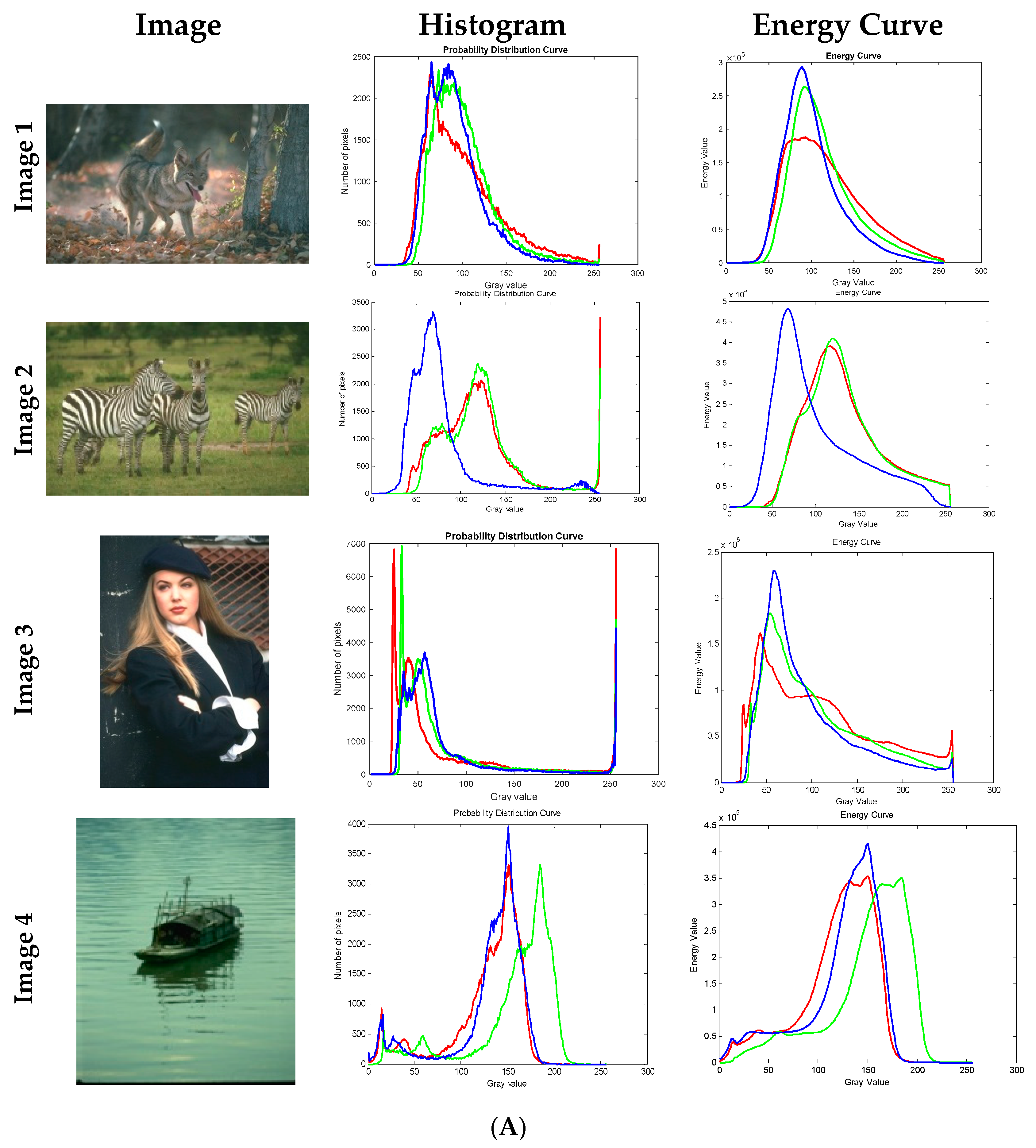
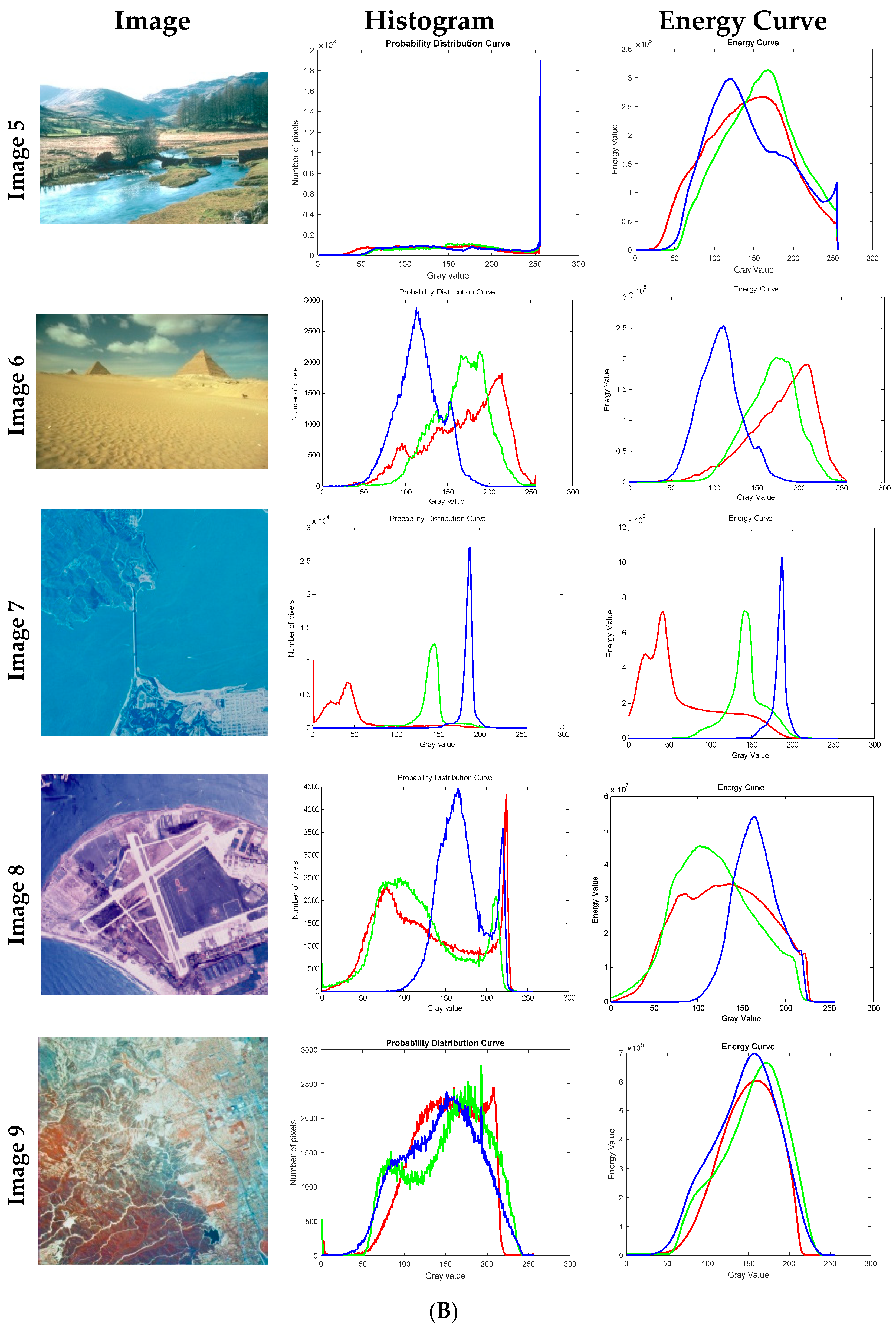
Figure 1.
(A) Images considered for experimentation along with histogram and energy curves of images. Red, green, and blue color plots indicate histograms and energy curves of red, green, and blue components of input images. (B) Images considered for experimentation along with histogram and energy curves of images. Red, green, and blue color plots indicate the histograms and energy curves of red, green, and blue components of input images.
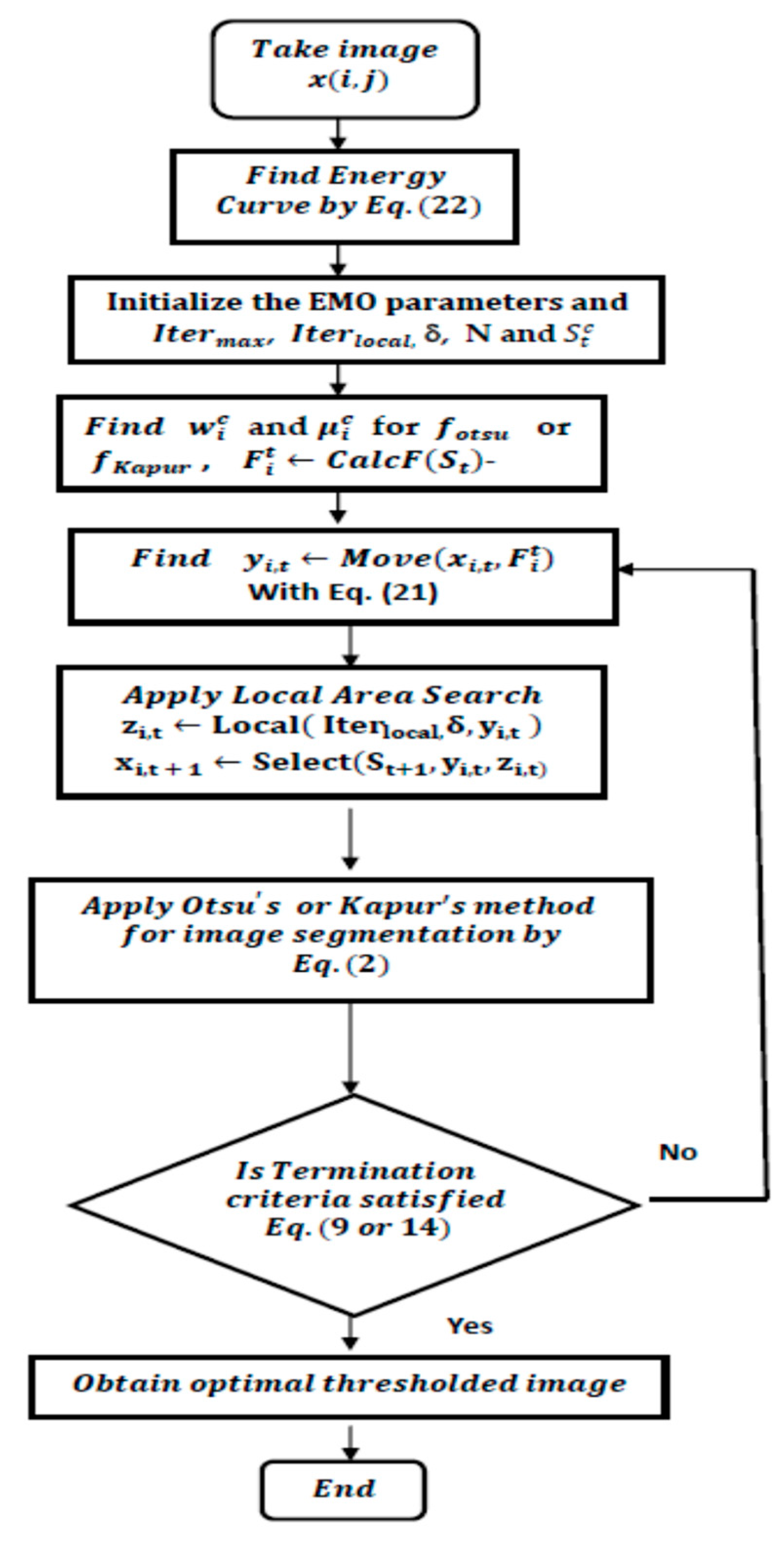
Figure 2.
Flow chart of the proposed approach to color image segmentation.
Figure 2.
Flow chart of the proposed approach to color image segmentation.
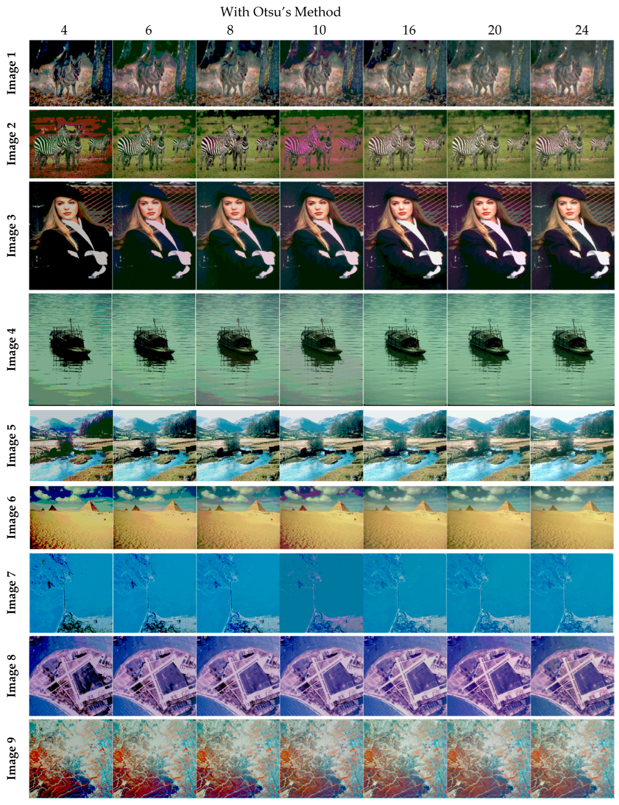
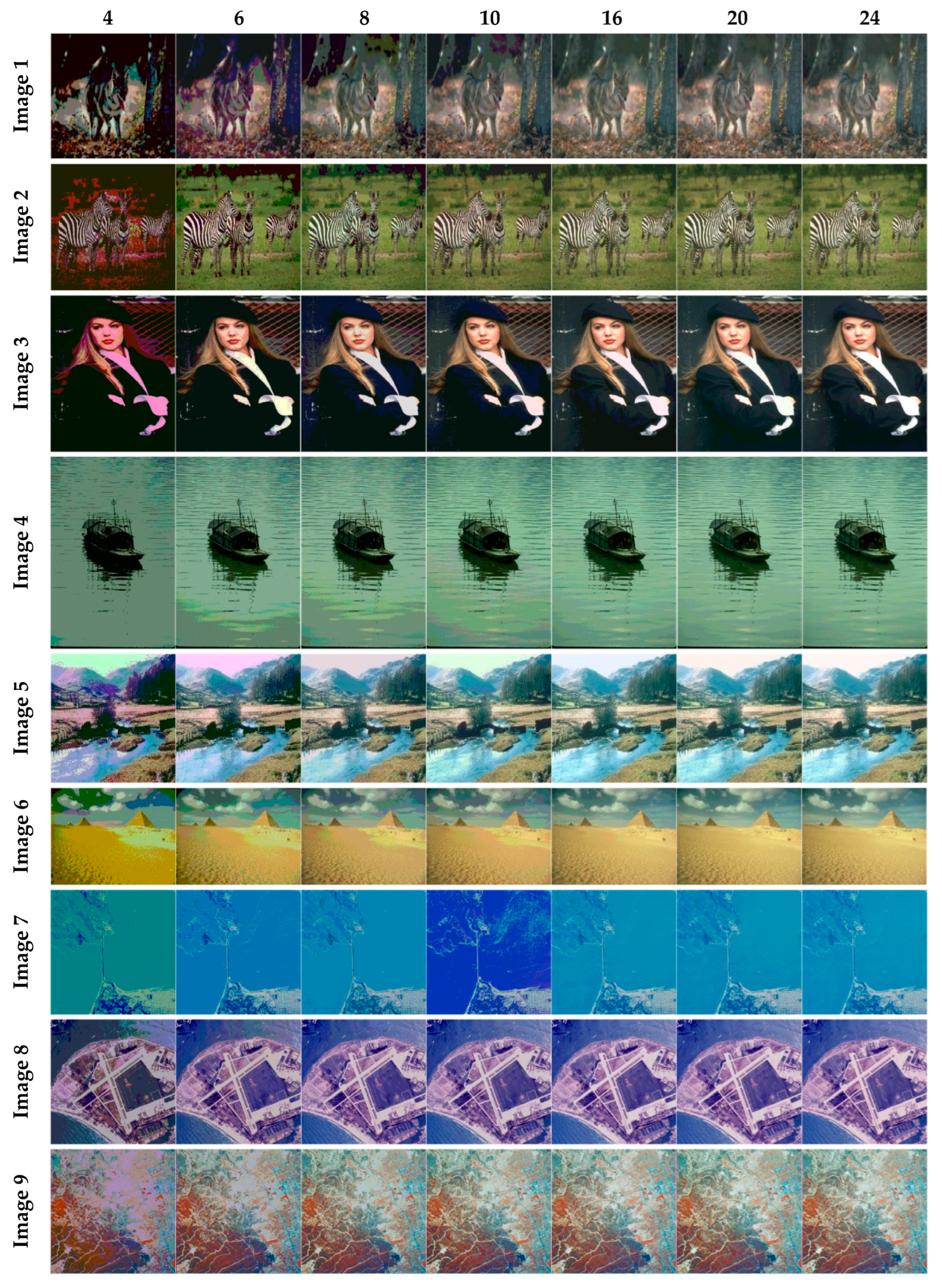
Figure 3.
Segmented images of Image 1 to Image 9 for N = 4, 6, 8, 10, 16, 20, and 24 using the proposed method based on Otsu’s method.
Figure 3.
Segmented images of Image 1 to Image 9 for N = 4, 6, 8, 10, 16, 20, and 24 using the proposed method based on Otsu’s method.
Figure 4.
Segmented images of Image 1 to Image 9 for N = 4, 6, 8, 10, 16, 20, and 24 using the proposed method based on Kapur’s method.
Figure 4.
Segmented images of Image 1 to Image 9 for N = 4, 6, 8, 10, 16, 20, and 24 using the proposed method based on Kapur’s method.
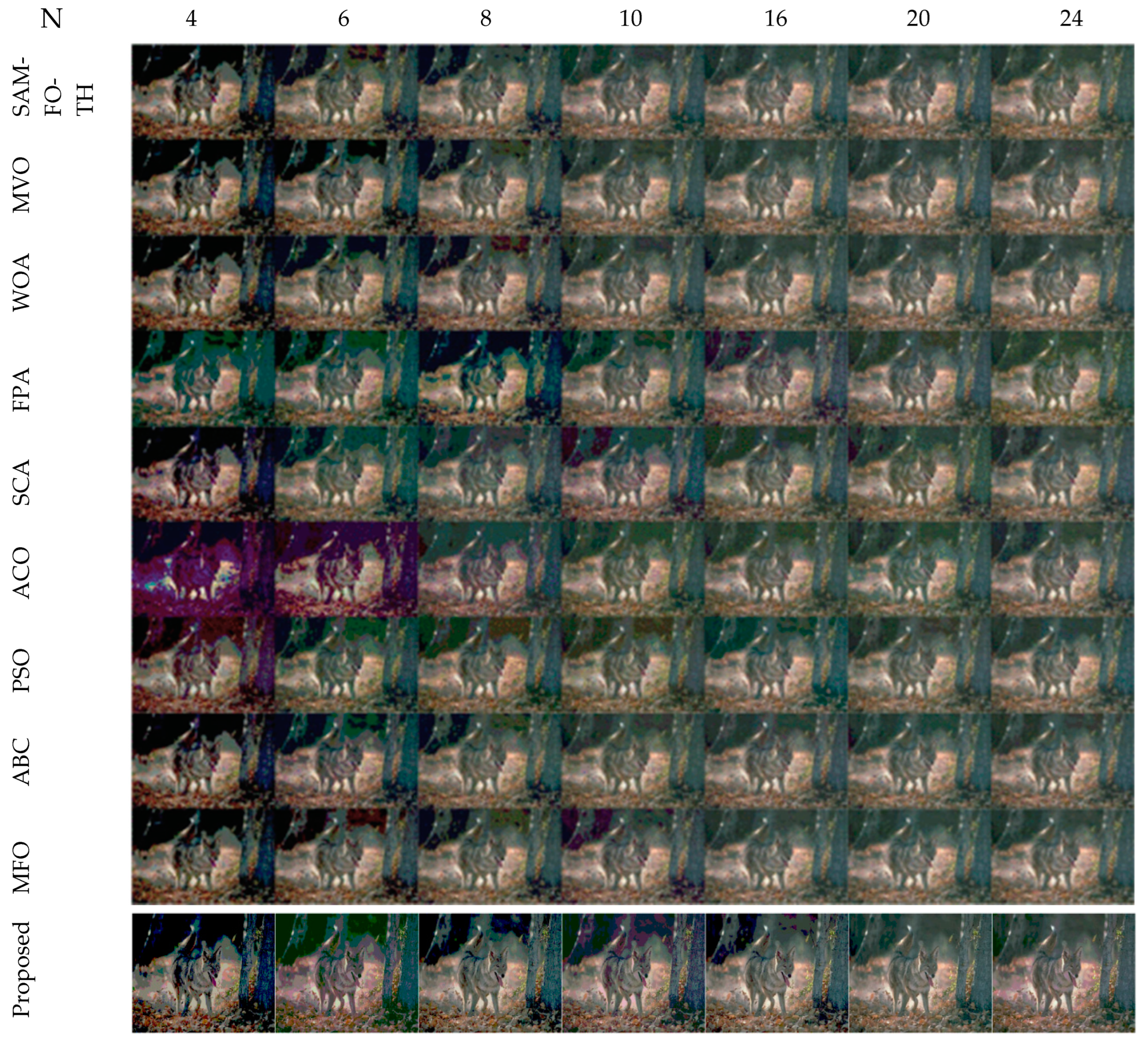
Figure 5.
Segmented images of Image 1 at N = 4, 6, 8, 10, 16, 20, and 24, using SAMFO-TH, MVO, WOA, FPA, SCA, ACO, PSO, ABC, and MFO, and with the proposed model based on Kapur’s method.
Figure 5.
Segmented images of Image 1 at N = 4, 6, 8, 10, 16, 20, and 24, using SAMFO-TH, MVO, WOA, FPA, SCA, ACO, PSO, ABC, and MFO, and with the proposed model based on Kapur’s method.
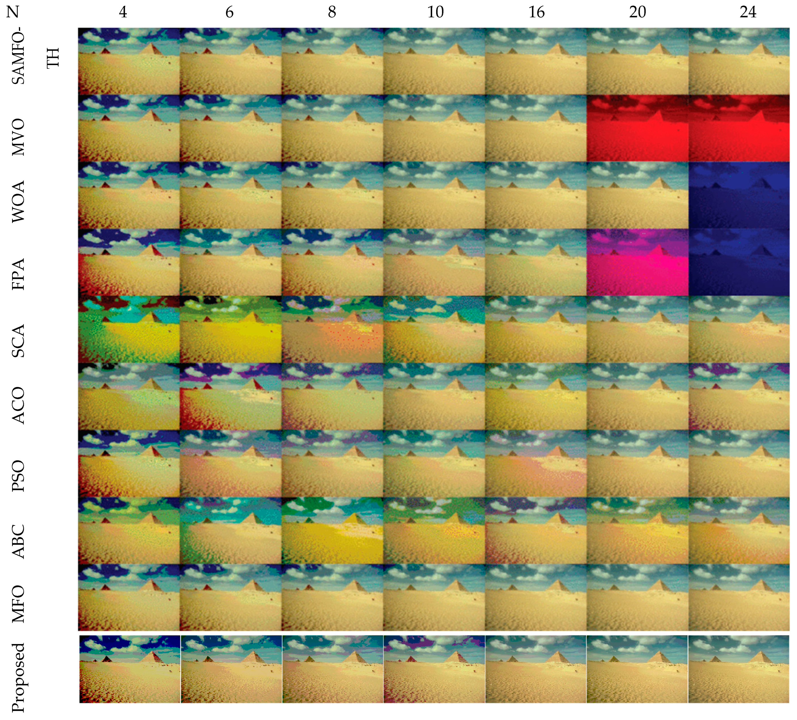
Figure 6.
Segmented images of Image 6 at N = 4, 6, 8, 10, 16, 20, and 24, using SAMFO-TH, MVO, WOA, FPA, SCA, ACO, PSO, ABC, and MFO, and with the proposed model based on Otsu’s method.
Figure 6.
Segmented images of Image 6 at N = 4, 6, 8, 10, 16, 20, and 24, using SAMFO-TH, MVO, WOA, FPA, SCA, ACO, PSO, ABC, and MFO, and with the proposed model based on Otsu’s method.
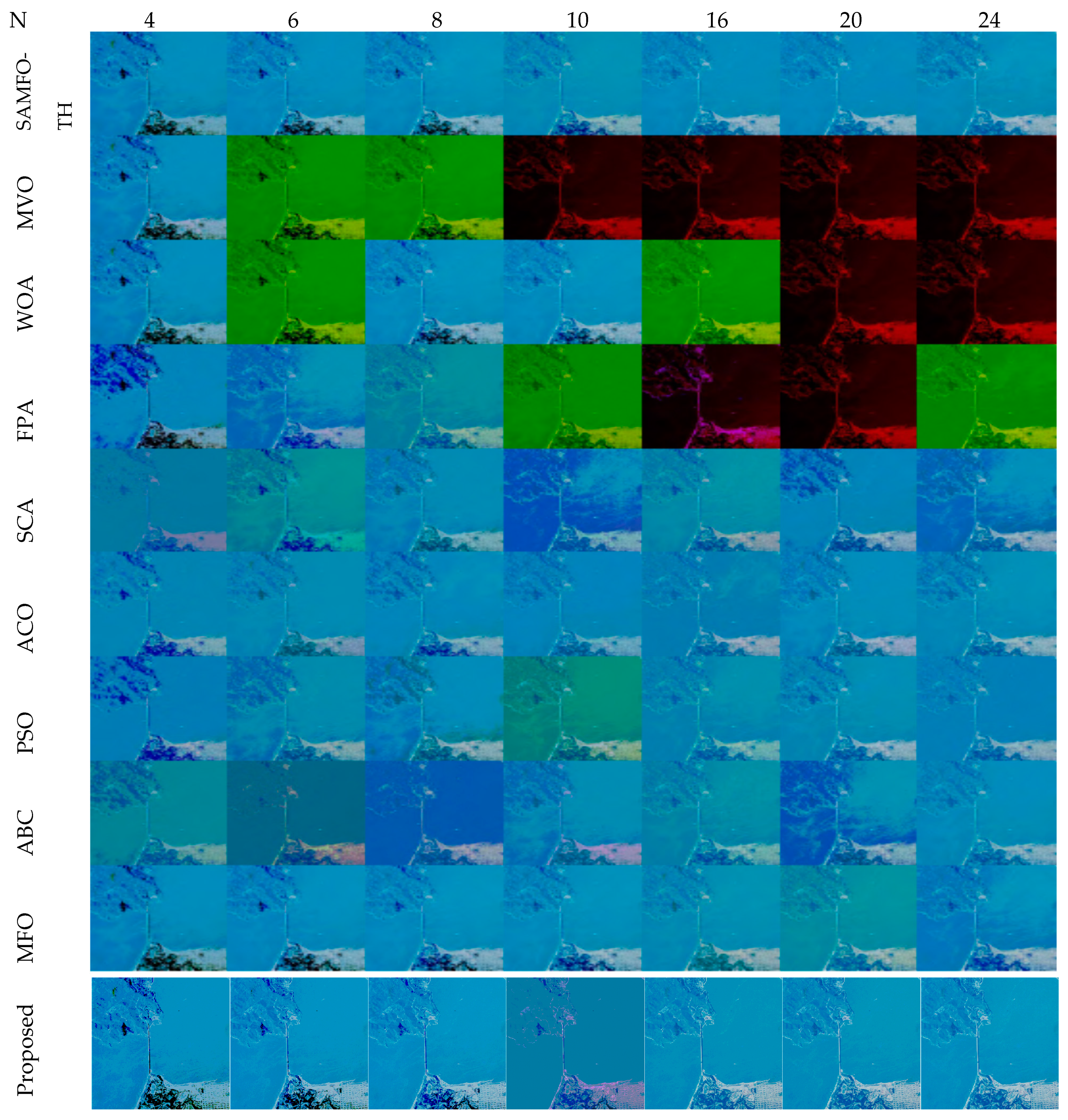
Figure 7.
Segmented images of Image 7 at N = 4, 6, 8, 10, 16, 20, and 24, using SAMFO-TH, MVO, WOA, FPA, SCA, ACO, PSO, ABC, and MFO, and with the proposed model based on Otsu’s method.
Figure 7.
Segmented images of Image 7 at N = 4, 6, 8, 10, 16, 20, and 24, using SAMFO-TH, MVO, WOA, FPA, SCA, ACO, PSO, ABC, and MFO, and with the proposed model based on Otsu’s method.
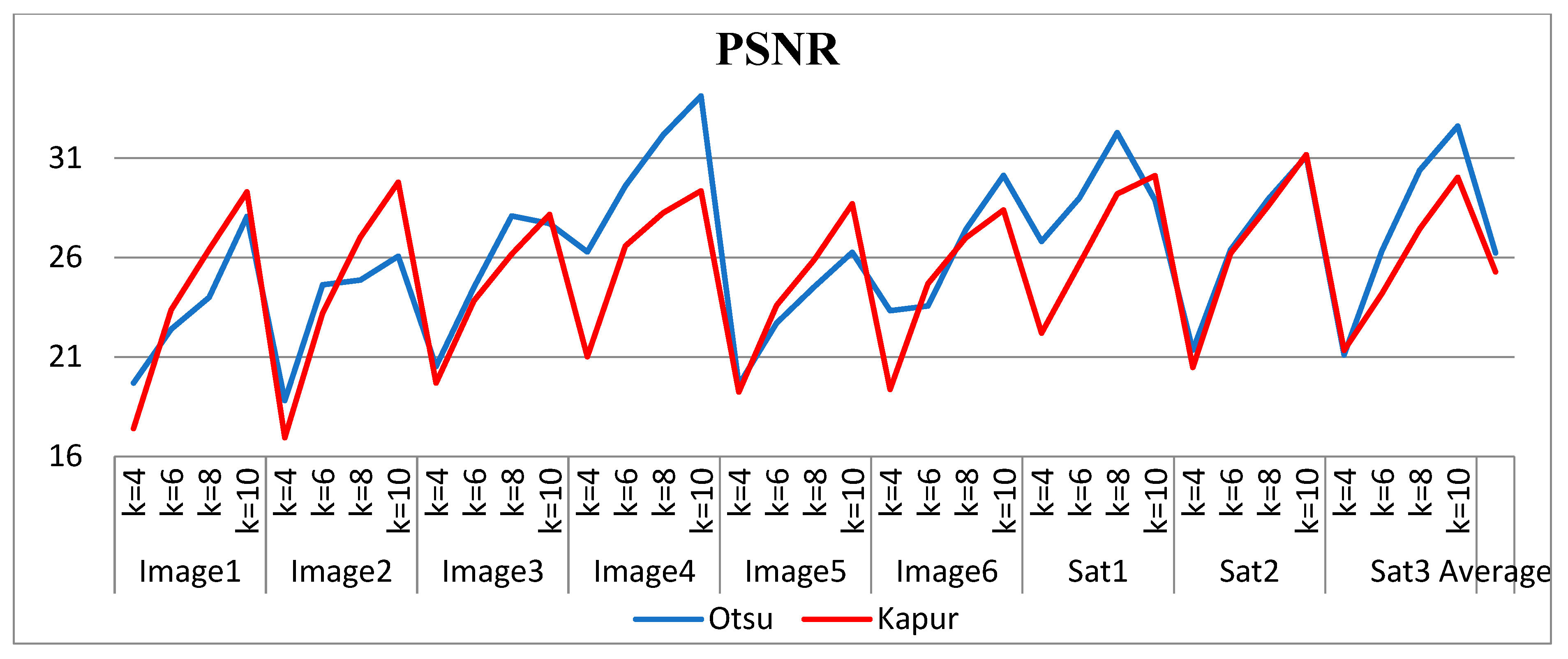
Figure 8.
Comparison of PSNR for the proposed method using Otsu’s and Kapur’s methods.
Figure 8.
Comparison of PSNR for the proposed method using Otsu’s and Kapur’s methods.
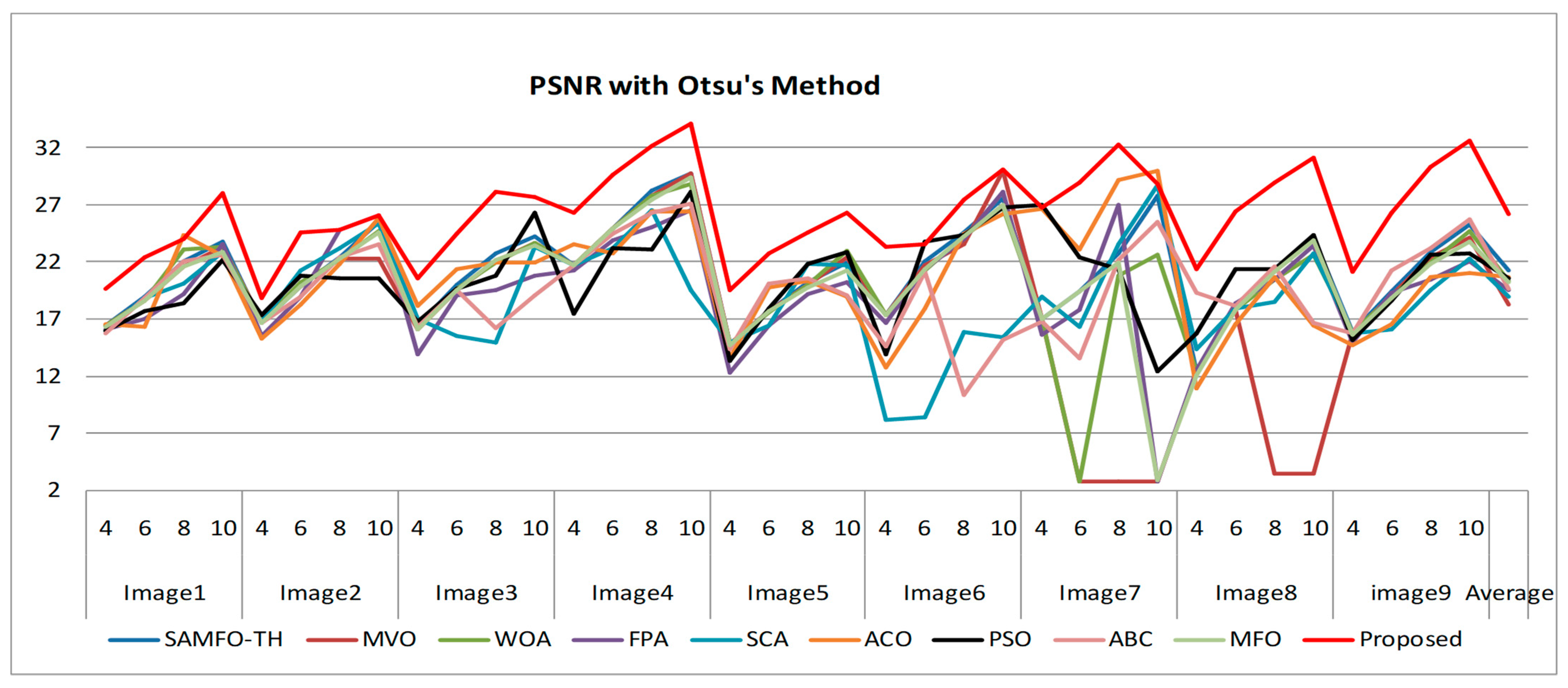
Figure 9.
Comparison of PSNR based on Otsu’s method.
Figure 9.
Comparison of PSNR based on Otsu’s method.
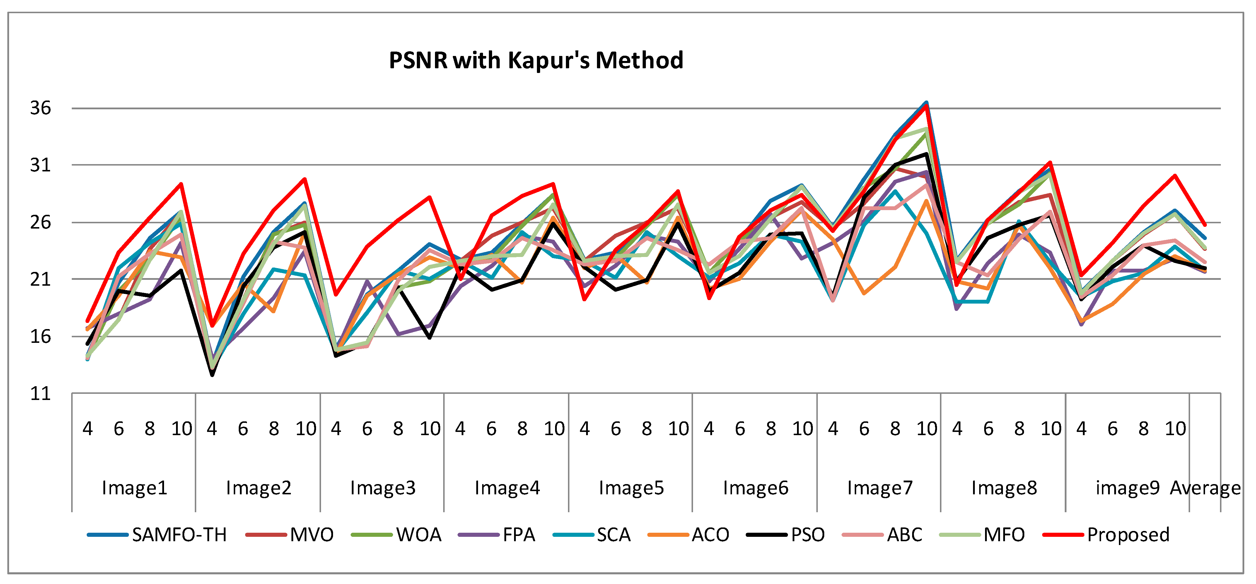
Figure 10.
Comparison of PSNR based on Kapur’s method.
Figure 10.
Comparison of PSNR based on Kapur’s method.
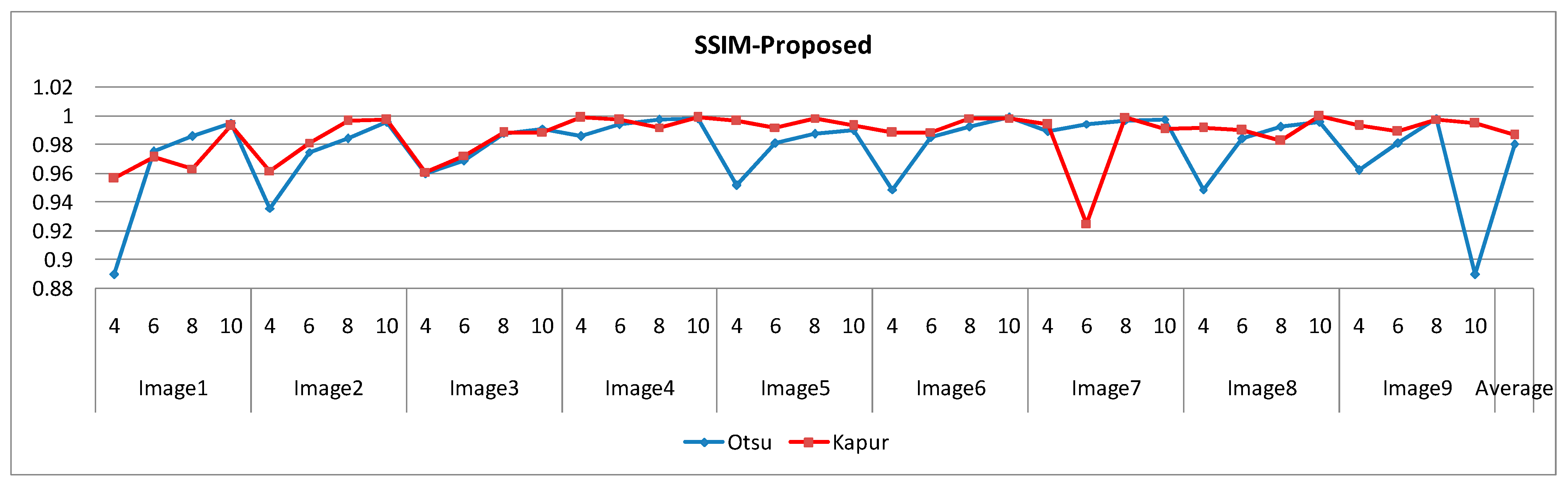
Figure 11.
Comparison of SSIM with the proposed method based on Otsu’s and Kapur’s criteria.
Figure 11.
Comparison of SSIM with the proposed method based on Otsu’s and Kapur’s criteria.
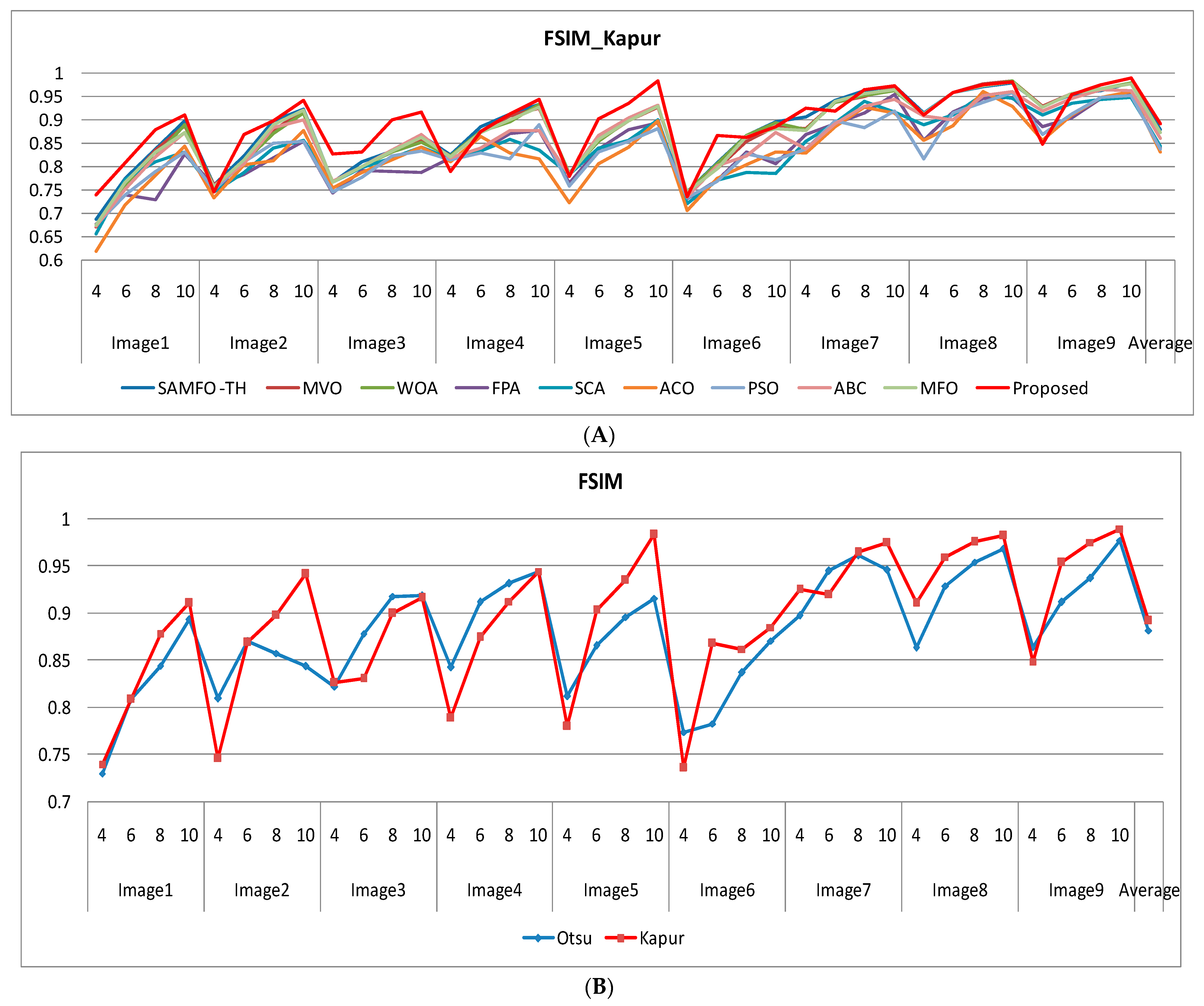
Figure 12.
(A) Comparison of PSNR based on Kapur’s method. (B) Comparison of FSIM with the proposed method based on Otsu’s and Kapur’scriteria.
Figure 12.
(A) Comparison of PSNR based on Kapur’s method. (B) Comparison of FSIM with the proposed method based on Otsu’s and Kapur’scriteria.
Table 1.
Different metrics to test the efficiency of the algorithms.
Table 1.
Different metrics to test the efficiency of the algorithms.
| S.No | Comparative
Parameters | Formula | Remarks |
|---|
| 1 | The mean value of fitness (MEAN) | It can be calculated as the average value of fitness values of objective values at each iteration of the algorithm. | Inter-class variance and entropy are the objective functions for Otsu’s and Kapur’s methods. |
| 3 | Peak signal-to-noise ratio (PSNR) | | The MAX is the maximum gray value taken as 255. |
| 4 | Mean square error (MSE) |
| is the input image and the segmented image is . is the size of the image. |
| 5 | Structural similarity (SSIM) | | and are the mean intensities of input and segmented images. is the covariance, and are the variance of images. |
| 6 | Feature similarity index (FSIM) | | is the similarity between images. is the maximum phase congruency of two images. |
| 7 | Probability Rand Index (PRI) | The internal validation measurePRIis an indication of resemblance between two regions in an image or clusters; it is expressed as given below
| Whereas dataset is portioned into two subsets and , the number of pairs of pixels (or elements) that are present in both subsets and is indicated by .
indicates the number of pairs of elements in X that are a different subset in C1 and a different subset in C2.
indicates the number of pairs of elements in X that are the same subset in C1 and a different subset in C2.
denotes the number of pairs of elements in X that are a different subset in C1 and the same subset in C2. |
| 8 | Variation of information (VOI) |
| is the segmented image, is the reference image, is entropy, is joint entropy. |
Table 2.
Comparison of PSNR computed by SAMFO-TH, MVO, WOA, FPA, SCA, ACO, PSO, ABC, and MFO with the proposed model using Kapur’s method with N = 4, 6, 8, and 10.
Table 2.
Comparison of PSNR computed by SAMFO-TH, MVO, WOA, FPA, SCA, ACO, PSO, ABC, and MFO with the proposed model using Kapur’s method with N = 4, 6, 8, and 10.
| Image | N | PSNR |
|---|
| | | SAMFO-TH | MVO | WOA | FPA | SCA | ACO | PSO | ABC | MFO | Proposed |
|---|
| Image 1 | 4 | 14.2867 | 14.2850 | 14.1218 | 16.6767 | 13.9373 | 16.6382 | 15.3040 | 14.1319 | 14.2850 | 17.411 |
| 6 | 0.7623 | 17.4474 | 20.0144 | 18.0251 | 22.0077 | 19.5418 | 19.9410 | 21.2326 | 17.4474 | 23.3624 |
| 8 | 24.5806 | 23.6349 | 22.7130 | 19.2523 | 24.1795 | 23.4068 | 19.5648 | 23.2057 | 22.6762 | 26.4105 |
| 10 | 26.9502 | 26.7858 | 26.4701 | 24.2091 | 25.8698 | 22.9264 | 21.8110 | 24.9282 | 26.8866 | 29.3038 |
| Image 2 | 4 | 13.5789 | 13.3799 | 13.2111 | 14.0750 | 13.1322 | 16.9569 | 12.6058 | 13.2116 | 13.3799 | 16.9332 |
| 6 | 21.2486 | 19.1958 | 19.1717 | 16.7705 | 18.0188 | 20.6228 | 20.3663 | 18.9082 | 19.2011 | 23.2135 |
| 8 | 25.1726 | 24.9161 | 24.9029 | 19.3409 | 21.8487 | 18.1980 | 23.7460 | 24.3227 | 24.1126 | 27.0255 |
| 10 | 27.6556 | 26.0105 | 25.7441 | 23.4190 | 21.3457 | 25.1496 | 25.1499 | 23.7446 | 27.4677 | 29.7932 |
| Image 3 | 4 | 14.9730 | 14.7516 | 14.7516 | 14.6601 | 14.6416 | 14.3734 | 14.3436 | 14.7839 | 14.8017 | 19.6832 |
| 6 | 19.6315 | 15.3583 | 15.3563 | 20.8057 | 18.0842 | 19.5661 | 15.4180 | 15.1249 | 15.4616 | 23.8255 |
| 8 | 21.8110 | 20.2832 | 20.2763 | 16.1667 | 21.7836 | 21.4141 | 20.3278 | 20.8963 | 19.9967 | 26.1728 |
| 10 | 24.0922 | 20.8407 | 20.7880 | 16.9484 | 21.0673 | 22.9669 | 15.8518 | 23.5685 | 22.0379 | 28.1644 |
| Image 4 | 4 | 22.6650 | 22.6187 | 22.6187 | 20.3850 | 22.5610 | 21.9843 | 22.1260 | 22.2906 | 22.5522 | 21.0083 |
| 6 | 23.3561 | 24.8435 | 22.8323 | 22.1698 | 21.1181 | 23.1694 | 20.0681 | 22.5925 | 23.0749 | 26.5867 |
| 8 | 25.8717 | 25.9515 | 25.6615 | 24.8007 | 25.1022 | 20.6755 | 20.9384 | 24.5891 | 23.1128 | 28.2479 |
| 10 | 28.3709 | 27.2012 | 28.3390 | 24.2414 | 22.9892 | 26.3917 | 25.8571 | 23.5946 | 27.5801 | 29.3581 |
| Image 5 | 4 | 22.6650 | 22.6187 | 22.6187 | 20.3850 | 22.5610 | 21.9843 | 22.1260 | 22.2906 | 22.5522 | 19.2267 |
| 6 | 23.3561 | 24.8435 | 22.8323 | 22.1698 | 21.1181 | 23.1694 | 20.0681 | 22.5925 | 23.0749 | 23.5926 |
| 8 | 25.8717 | 25.9515 | 25.6615 | 24.8007 | 25.1022 | 20.6755 | 20.9384 | 24.5891 | 23.1128 | 25.8969 |
| 10 | 28.3709 | 27.2012 | 28.3390 | 24.2414 | 22.9892 | 26.3917 | 25.8571 | 23.5946 | 27.5801 | 28.7066 |
| Image 6 | 4 | 21.5290 | 21.5290 | 21.5290 | 20.8569 | 21.0864 | 20.1992 | 19.9682 | 22.2765 | 21.5068 | 19.3631 |
| 6 | 24.3622 | 24.3605 | 24.3905 | 23.6272 | 22.4015 | 21.0277 | 21.5290 | 24.3142 | 23.0741 | 24.6747 |
| 8 | 27.8633 | 26.4006 | 26.2061 | 26.7374 | 24.9330 | 24.2707 | 24.8640 | 24.5837 | 26.2940 | 26.9835 |
| 10 | 29.1790 | 27.7527 | 29.1194 | 22.7830 | 24.2800 | 27.0600 | 25.0170 | 27.2259 | 29.0730 | 28.3946 |
| Image 7 | 4 | 25.5470 | 25.4570 | 25.4570 | 24.1766 | 19.1235 | 24.5240 | 19.4536 | 19.0881 | 25.4570 | 25.195 |
| 6 | 29.7362 | 27.6434 | 28.9754 | 26.1089 | 25.7468 | 19.7999 | 28.1928 | 27.1875 | 28.9557 | 28.6755 |
| 8 | 33.6300 | 30.7366 | 30.6802 | 29.5335 | 28.6656 | 22.0921 | 30.9938 | 27.1974 | 33.3217 | 33.1943 |
| 10 | 36.4519 | 29.9769 | 33.7857 | 30.3995 | 24.9723 | 27.8741 | 31.9742 | 29.1914 | 34.1678 | 36.1217 |
| Image 8 | 4 | 22.6392 | 22.5244 | 22.5244 | 18.4377 | 19.0066 | 20.8646 | 20.8291 | 22.5279 | 22.5244 | 20.4749 |
| 6 | 26.1655 | 25.8536 | 25.8350 | 22.4239 | 19.0136 | 20.1567 | 24.5617 | 21.3842 | 25.8134 | 26.2102 |
| 8 | 28.6575 | 27.7273 | 27.5732 | 24.9561 | 26.0938 | 25.7541 | 25.7131 | 24.5071 | 28.6420 | 28.6113 |
| 10 | 30.5915 | 28.401 | 30.2800 | 23.3037 | 22.4820 | 21.9794 | 26.6112 | 26.8636 | 30.2009 | 31.1743 |
| Image 9 | 4 | 19.8193 | 19.7421 | 19.7421 | 17.0760 | 19.4905 | 17.2988 | 19.2776 | 19.4984 | 19.8087 | 21.3238 |
| 6 | 22.6291 | 22.5596 | 22.6157 | 21.7415 | 20.7706 | 18.7977 | 22.0371 | 21.3628 | 22.6060 | 24.1806 |
| 8 | 25.1702 | 24.9523 | 25.0680 | 21.7143 | 21.5330 | 21.4059 | 23.9504 | 23.9585 | 25.0186 | 27.439 |
| 10 | 27.0309 | 26.7189 | 26.6886 | 22.8024 | 23.8913 | 23.0109 | 22.6262 | 24.3817 | 26.6501 | 30.0399 |
| Average | | 24.6188 | 23.6325 | 23.8026 | 21.6728 | 21.7482 | 21.7316 | 21.9444 | 22.4984 | 23.7086 | 25.7213 |
Table 3.
Comparison of MSE computed by SAMFO-TH, MVO, WOA, FPA, SCA, ACO, PSO, ABC, and MFO with the proposed model using Kapur’s method with N = 4, 6, 8, and 10.
Table 3.
Comparison of MSE computed by SAMFO-TH, MVO, WOA, FPA, SCA, ACO, PSO, ABC, and MFO with the proposed model using Kapur’s method with N = 4, 6, 8, and 10.
| Image | N | MSE-Kapur |
|---|
| | | SAMFO-TH | MVO | WOA | FPA | SCA | ACO | PSO | ABC | MFO | Proposed |
|---|
| Image 1 | 4 | 2423.32 | 2424.22 | 2517.14 | 1397.72 | 2626.34 | 1410.17 | 1917.33 | 2511.23 | 2424.28 | 1183.26 |
| 6 | 545.564 | 1170.47 | 648.102 | 1024.60 | 409.55 | 722.602 | 659.140 | 489.575 | 1170.47 | 299.806 |
| 8 | 197.301 | 281.571 | 348.158 | 772.419 | 226.473 | 296.753 | 718.782 | 310.824 | 351.125 | 148.604 |
| 10 | 131.237 | 136.302 | 146.579 | 246.702 | 168.305 | 331.467 | 428.533 | 209.054 | 133.175 | 76.3309 |
| Image 2 | 4 | 2956.02 | 2986.04 | 3104.45 | 2544.33 | 3161.27 | 1310.45 | 3568.64 | 3104.05 | 2986.03 | 1317.53 |
| 6 | 355.465 | 782.530 | 786.885 | 1367.80 | 1026.15 | 487.773 | 597.653 | 836.101 | 781.568 | 310.2633 |
| 8 | 197.617 | 209.639 | 210.277 | 756.819 | 424.825 | 984.645 | 274.458 | 240.330 | 252.243 | 128.9824 |
| 10 | 111.562 | 162.940 | 173.249 | 295.925 | 476.991 | 198.665 | 198.650 | 274.547 | 116.495 | 68.19623 |
| Image 3 | 4 | 2152.35 | 2177.33 | 2177.33 | 2223.71 | 2233.28 | 2375.45 | 1899.97 | 2151.26 | 2152.30 | 699.4559 |
| 6 | 707.825 | 1893.42 | 1894.34 | 540.146 | 1010.88 | 718.566 | 1867.60 | 1998.01 | 1848.93 | 269.4824 |
| 8 | 428.524 | 609.199 | 610.169 | 1571.85 | 431.236 | 469.541 | 602.970 | 528.995 | 650.742 | 156.9641 |
| 10 | 253.433 | 535.808 | 542.347 | 1312.95 | 508.565 | 328.393 | 1690.17 | 285.908 | 406.716 | 99.2294 |
| Image 4 | 4 | 352.032 | 355.804 | 355.804 | 595.089 | 336.500 | 411.762 | 316.575 | 383.729 | 361.295 | 515.5257 |
| 6 | 300.242 | 213.170 | 338.727 | 394.552 | 502.651 | 313.429 | 640.131 | 357.955 | 320.322 | 142.6955 |
| 8 | 168.231 | 165.168 | 176.575 | 215.281 | 159.537 | 556.585 | 523.894 | 226.032 | 317.543 | 97.33978 |
| 10 | 94.6216 | 123.869 | 95.3183 | 244.874 | 326.710 | 149.250 | 168.800 | 284.196 | 113.518 | 75.38247 |
| Image 5 | 4 | 1525.07 | 1529.68 | 1529.63 | 2356.50 | 1356.78 | 1662.81 | 1220.39 | 1689.70 | 1558.81 | 776.9809 |
| 6 | 623.770 | 650.887 | 636.915 | 634.497 | 469.579 | 1258.92 | 702.469 | 441.362 | 666.638 | 284.3285 |
| 8 | 325.161 | 343.619 | 335.542 | 425.048 | 553.578 | 861.665 | 568.193 | 357.963 | 326.081 | 167.2593 |
| 10 | 195.209 | 237.657 | 205.215 | 407.361 | 330.530 | 264.978 | 529.601 | 203.436 | 236.277 | 87.58311 |
| Image 6 | 4 | 457.273 | 457.273 | 457.273 | 533.814 | 506.337 | 621.104 | 655.032 | 384.975 | 459.617 | 752.9573 |
| 6 | 236.608 | 238.250 | 320.382 | 282.072 | 374.051 | 513.229 | 457.273 | 240.802 | 238.152 | 221.6207 |
| 8 | 106.353 | 148.943 | 155.764 | 137.829 | 208.824 | 243.228 | 212.170 | 226.312 | 152.644 | 130.2358 |
| 10 | 78.5562 | 109.097 | 79.6421 | 342.597 | 242.706 | 127.961 | 204.821 | 123.164 | 80.4963 | 94.10666 |
| Image 7 | 4 | 185.090 | 185.090 | 185.090 | 248.551 | 795.662 | 229.447 | 737.426 | 802.177 | 185.090 | 392.2657 |
| 6 | 69.0973 | 111.875 | 82.3258 | 159.289 | 173.142 | 680.915 | 98.5827 | 124.258 | 82.7000 | 176.0072 |
| 8 | 28.1892 | 54.8811 | 55.5983 | 72.3988 | 88.4136 | 401.668 | 51.7245 | 123.975 | 30.2638 | 78.27992 |
| 10 | 14.7190 | 65.3712 | 27.1964 | 59.3091 | 206.943 | 106.089 | 41.2723 | 78.3322 | 62.5614 | 63.22813 |
| Image 8 | 4 | 354.124 | 363.613 | 363.613 | 931.783 | 817.366 | 532.874 | 537.243 | 363.320 | 363.613 | 582.895 |
| 6 | 157.227 | 168.935 | 169.662 | 372.125 | 816.056 | 627.207 | 227.463 | 472.784 | 170.506 | 155.6182 |
| 8 | 25.7542 | 88.5788 | 113.698 | 207.717 | 159.844 | 109.735 | 174.491 | 230.341 | 88.8945 | 89.52624 |
| 10 | 62.0859 | 93.9654 | 60.9653 | 303.882 | 367.180 | 412.227 | 141.894 | 133.882 | 56.7455 | 49.61927 |
| Image 9 | 4 | 677.871 | 690.033 | 690.033 | 1274.95 | 731.182 | 1211.21 | 767.929 | 729.868 | 679.526 | 479.4026 |
| 6 | 354.950 | 360.679 | 356.051 | 435.445 | 544.529 | 857.653 | 406.786 | 475.113 | 356.846 | 248.325 |
| 8 | 197.722 | 207.897 | 202.433 | 438.178 | 456.855 | 470.421 | 261.845 | 261.355 | 204.750 | 117.2682 |
| 10 | 128.822 | 138.417 | 139.384 | 341.065 | 265.432 | 325.078 | 355.185 | 237.088 | 140.626 | 64.43033 |
| Average | | 477.194 | 568.672 | 563.662 | 707.477 | 652.618 | 627.331 | 678.474 | 608.111 | 70.219 | 294.4718 |
Table 4.
Comparison of SSIM computed by SAMFO-TH, MVO, WOA, FPA, SCA, ACO, PSO, ABC, and MFO with the proposed model using Kapur’s method with N = 4, 6, 8, and 10.
Table 4.
Comparison of SSIM computed by SAMFO-TH, MVO, WOA, FPA, SCA, ACO, PSO, ABC, and MFO with the proposed model using Kapur’s method with N = 4, 6, 8, and 10.
| Image | N | SSIM-Kapur |
|---|
| | | SAMFO-TH | MVO | WOA | FPA | SCA | ACO | PSO | ABC | MFO | Proposed |
|---|
| Image 1 | 4 | 0.9275 | 0.9190 | 0.9209 | 0.9206 | 0.9016 | 0.8788 | 0.9193 | 0.9146 | 0.9213 | 0.9568 |
| 6 | 0.9768 | 0.9600 | 0.9652 | 0.9624 | 0.9758 | 0.9419 | 0.9723 | 0.9681 | 0.9653 | 0.9713 |
| 8 | 0.9882 | 0.9858 | 0.9830 | 0.9389 | 0.9860 | 0.9877 | 0.9837 | 0.9861 | 0.9852 | 0.9636 |
| 10 | 0.9958 | 0.9947 | 0.9952 | 0.9879 | 0.9885 | 0.9927 | 0.9914 | 0.9949 | 0.9908 | 0.9932 |
| Image 2 | 4 | 0.9386 | 0.9353 | 0.9339 | 0.9475 | 0.9295 | 0.9353 | 0.9305 | 0.9357 | 0.9357 | 0.9619 |
| 6 | 0.9785 | 0.9735 | 0.9731 | 0.9634 | 0.9636 | 0.9662 | 0.9762 | 0.9738 | 0.9741 | 0.9815 |
| 8 | 0.9935 | 0.9874 | 0.9861 | 0.9794 | 0.9878 | 0.9790 | 0.9896 | 0.9924 | 0.9920 | 0.9967 |
| 10 | 0.9953 | 0.9951 | 0.9944 | 0.9850 | 0.9894 | 0.9907 | 0.9876 | 0.9934 | 0.9952 | 0.9971 |
| Image 3 | 4 | 0.9417 | 0.9393 | 0.9395 | 0.9382 | 0.9404 | 0.9332 | 0.9397 | 0.9390 | 0.9397 | 0.961 |
| 6 | 0.9611 | 0.9460 | 0.9464 | 0.9733 | 0.9549 | 0.9649 | 0.9559 | 0.9432 | 0.9490 | 0.9724 |
| 8 | 0.9785 | 0.9673 | 0.9662 | 0.9572 | 0.9713 | 0.9615 | 0.9726 | 0.9766 | 0.9675 | 0.9881 |
| 10 | 0.9890 | 0.9772 | 0.9725 | 0.9694 | 0.9853 | 0.9809 | 0.9722 | 0.9882 | 0.9770 | 0.9888 |
| Image 4 | 4 | 0.9886 | 0.9881 | 0.9881 | 0.9873 | 0.9876 | 0.9878 | 0.9879 | 0.9885 | 0.9879 | 0.9988 |
| 6 | 0.9942 | 0.9932 | 0.9934 | 0.9897 | 0.9905 | 0.9922 | 0.9873 | 0.9904 | 0.9939 | 0.9971 |
| 8 | 0.9959 | 0.9951 | 0.9959 | 0.9938 | 0.9919 | 0.9877 | 0.9883 | 0.9934 | 0.9955 | 0.9921 |
| 10 | 0.9973 | 0.9971 | 0.9972 | 0.9924 | 0.9910 | 0.9894 | 0.9951 | 0.9943 | 0.9970 | 0.999 |
| Image 5 | 4 | 0.9699 | 0.9695 | 0.9695 | 0.9632 | 0.9638 | 0.9606 | 0.9695 | 0.9658 | 0.9691 | 0.9964 |
| 6 | 0.9869 | 0.9858 | 0.9865 | 0.9817 | 0.9836 | 0.9789 | 0.9855 | 0.9894 | 0.9863 | 0.9921 |
| 8 | 0.9916 | 0.9915 | 0.9914 | 0.9910 | 0.9872 | 0.9859 | 0.9833 | 0.9918 | 0.9911 | 0.9986 |
| 10 | 0.9952 | 0.9949 | 0.9945 | 0.9936 | 0.9932 | 0.9920 | 0.9917 | 0.9953 | 0.9943 | 0.9934 |
| Image 6 | 4 | 0.9887 | 0.9887 | 0.9887 | 0.9870 | 0.9837 | 0.9826 | 0.9766 | 0.9874 | 0.9888 | 0.9885 |
| 6 | 0.9935 | 0.9927 | 0.9935 | 0.9899 | 0.9906 | 0.9885 | 0.9903 | 0.9930 | 0.9931 | 0.98871 |
| 8 | 0.9965 | 0.9960 | 0.9957 | 0.9950 | 0.9918 | 0.9928 | 0.9934 | 0.9945 | 0.9959 | 0.9984 |
| 10 | 0.9978 | 0.9973 | 0.9975 | 0.9935 | 0.9921 | 0.9932 | 0.9929 | 0.9968 | 0.9975 | 0.9986 |
| Image 7 | 4 | 0.9915 | 0.9811 | 0.9811 | 0.9810 | 0.9768 | 0.9768 | 0.9730 | 0.9759 | 0.9809 | 0.9939 |
| 6 | 0.9950 | 0.9946 | 0.9946 | 0.9838 | 0.9883 | 0.9903 | 0.9913 | 0.9931 | 0.9948 | 0.9252 |
| 8 | 0.9971 | 0.9954 | 0.9959 | 0.9932 | 0.9952 | 0.9956 | 0.9888 | 0.9947 | 0.9958 | 0.9994 |
| 10 | 0.9980 | 0.9977 | 0.9964 | 0.9972 | 0.9956 | 0.9948 | 0.9927 | 0.9973 | 0.9976 | 0.9908 |
| Image 8 | 4 | 0.9855 | 0.9853 | 0.9853 | 0.9771 | 0.9797 | 0.9796 | 0.9799 | 0.9851 | 0.9853 | 0.9918 |
| 6 | 0.9932 | 0.9930 | 0.9929 | 0.9900 | 0.9840 | 0.9820 | 0.9850 | 0.9899 | 0.9931 | 0.9899 |
| 8 | 0.9961 | 0.9956 | 0.9954 | 0.9912 | 0.9939 | 0.9905 | 0.9936 | 0.9918 | 0.9954 | 0.9829 |
| 10 | 0.9974 | 0.9969 | 0.9971 | 0.9934 | 0.9920 | 0.9909 | 0.9949 | 0.9946 | 0.9971 | 0.9995 |
| Image 9 | 4 | 0.9799 | 0.9795 | 0.9795 | 0.9735 | 0.9774 | 0.9708 | 0.9744 | 0.9742 | 0.9796 | 0.993 |
| 6 | 0.9902 | 0.9898 | 0.9895 | 0.9767 | 0.9805 | 0.9816 | 0.9857 | 0.9881 | 0.9892 | 0.9892 |
| 8 | 0.9935 | 0.9934 | 0.9933 | 0.9843 | 0.9903 | 0.9895 | 0.9922 | 0.9933 | 0.9932 | 0.9976 |
| 10 | 0.9963 | 0.9962 | 0.9961 | 0.9918 | 0.9855 | 0.9926 | 0.9920 | 0.9938 | 0.9962 | 0.9948 |
| Average | | 0.98539 | 0.982472 | 0.98237 | 0.97811 | 0.97945 | 0.97720 | 0.97989 | 0.98217 | 0.98281 | 0.9867 |
Table 5.
Comparison of FSIM computed by SAMFO-TH, MVO, WOA, FPA, SCA, ACO, PSO, ABC, and MFO with the proposed model using Kapur’s method with N = 4, 6, 8, and 10.
Table 5.
Comparison of FSIM computed by SAMFO-TH, MVO, WOA, FPA, SCA, ACO, PSO, ABC, and MFO with the proposed model using Kapur’s method with N = 4, 6, 8, and 10.
| Image | N | FSIM |
|---|
| | | SAMFO-TH | MVO | WOA | FPA | SCA | ACO | PSO | ABC | MFO | Proposed |
|---|
| Image 1 | 4 | 0.6875 | 0.6716 | 0.6749 | 0.6783 | 0.6558 | 0.6183 | 0.6754 | 0.6725 | 0.6754 | 0.74 |
| 6 | 0.7756 | 0.7626 | 0.7607 | 0.7405 | 0.7728 | 0.7182 | 0.7392 | 0.7532 | 0.7679 | 0.8089 |
| 8 | 0.8377 | 0.8365 | 0.8217 | 0.7294 | 0.8117 | 0.7807 | 0.7907 | 0.8218 | 0.8319 | 0.8787 |
| 10 | 0.8988 | 0.8890 | 0.8903 | 0.8268 | 0.8315 | 0.8444 | 0.8313 | 0.8727 | 0.8733 | 0.9108 |
| Image | 4 | 0.7613 | 0.7611 | 0.7597 | 0.7578 | 0.7452 | 0.7329 | 0.7496 | 0.7590 | 0.7563 | 0.7461 |
| 6 | 0.8234 | 0.8114 | 0.8109 | 0.7829 | 0.7881 | 0.8038 | 0.8111 | 0.8077 | 0.8150 | 0.8696 |
| 8 | 0.8982 | 0.8769 | 0.8704 | 0.8184 | 0.8409 | 0.8127 | 0.8499 | 0.8835 | 0.8910 | 0.8978 |
| 10 | 0.9233 | 0.9206 | 0.9153 | 0.8541 | 0.8561 | 0.8782 | 0.8540 | 0.9007 | 0.9216 | 0.9421 |
| Image | 4 | 0.7674 | 0.7664 | 0.7662 | 0.7441 | 0.7665 | 0.7537 | 0.7469 | 0.7681 | 0.7670 | 0.8265 |
| 6 | 0.8118 | 0.8001 | 0.7997 | 0.7927 | 0.7977 | 0.7878 | 0.7765 | 0.7995 | 0.8005 | 0.8310 |
| 8 | 0.8344 | 0.8326 | 0.8324 | 0.7906 | 0.8188 | 0.8149 | 0.8230 | 0.8355 | 0.8330 | 0.9001 |
| 10 | 0.8663 | 0.8561 | 0.8517 | 0.7883 | 0.8428 | 0.8417 | 0.8339 | 0.8691 | 0.8629 | 0.9168 |
| Image 4 | 4 | 0.8245 | 0.8241 | 0.8242 | 0.8196 | 0.8161 | 0.8114 | 0.8149 | 0.8183 | 0.8205 | 0.7890 |
| 6 | 0.8852 | 0.8756 | 0.8746 | 0.8334 | 0.8330 | 0.8650 | 0.8300 | 0.8391 | 0.8726 | 0.8751 |
| 8 | 0.9122 | 0.9094 | 0.8972 | 0.8718 | 0.8583 | 0.8294 | 0.8176 | 0.8775 | 0.9003 | 0.9129 |
| 10 | 0.9349 | 0.9246 | 0.9341 | 0.8766 | 0.8367 | 0.8171 | 0.8906 | 0.8766 | 0.9283 | 0.9446 |
| Image 5 | 4 | 0.7856 | 0.7854 | 0.7854 | 0.7641 | 0.7842 | 0.7222 | 0.7585 | 0.7809 | 0.7842 | 0.7800 |
| 6 | 0.8603 | 0.8576 | 0.8551 | 0.8370 | 0.8397 | 0.8069 | 0.8318 | 0.8678 | 0.8596 | 0.9032 |
| 8 | 0.9010 | 0.8983 | 0.9007 | 0.8793 | 0.8568 | 0.8419 | 0.8550 | 0.9038 | 0.8993 | 0.9350 |
| 10 | 0.9308 | 0.9287 | 0.9305 | 0.8953 | 0.9008 | 0.8995 | 0.8811 | 0.9311 | 0.9306 | 0.9834 |
| Image 6 | 4 | 0.7456 | 0.7454 | 0.7454 | 0.7311 | 0.7209 | 0.7069 | 0.7327 | 0.7359 | 0.7453 | 0.7363 |
| 6 | 0.8079 | 0.7953 | 0.8077 | 0.7717 | 0.7710 | 0.7751 | 0.7684 | 0.8032 | 0.7963 | 0.8682 |
| 8 | 0.8682 | 0.8544 | 0.8662 | 0.8326 | 0.7871 | 0.8044 | 0.8282 | 0.8236 | 0.8659 | 0.8621 |
| 10 | 0.8965 | 0.8862 | 0.8946 | 0.8066 | 0.7853 | 0.8316 | 0.8154 | 0.8731 | 0.8828 | 0.8851 |
| Image 7 | 4 | 0.9068 | 0.8824 | 0.8792 | 0.8687 | 0.8546 | 0.8298 | 0.8384 | 0.8384 | 0.8774 | 0.9252 |
| 6 | 0.9418 | 0.9377 | 0.9376 | 0.8928 | 0.8940 | 0.8857 | 0.8980 | 0.8921 | 0.9400 | 0.9198 |
| 8 | 0.9623 | 0.9500 | 0.9537 | 0.9161 | 0.9393 | 0.9279 | 0.8830 | 0.9298 | 0.9569 | 0.9647 |
| 10 | 0.9732 | 0.9707 | 0.9633 | 0.9553 | 0.9182 | 0.9146 | 0.9186 | 0.9442 | 0.9657 | 0.9746 |
| Image 8 | 4 | 0.9160 | 0.9139 | 0.9139 | 0.8562 | 0.8902 | 0.8572 | 0.8179 | 0.9099 | 0.9139 | 0.9111 |
| 6 | 0.9593 | 0.9591 | 0.9592 | 0.9170 | 0.9100 | 0.8888 | 0.9158 | 0.9004 | 0.9589 | 0.9599 |
| 8 | 0.9716 | 0.9772 | 0.9740 | 0.9472 | 0.9555 | 0.9605 | 0.9378 | 0.9537 | 0.9736 | 0.9759 |
| 10 | 0.9805 | 0.9849 | 0.9846 | 0.9479 | 0.9473 | 0.9299 | 0.9595 | 0.9620 | 0.9812 | 0.9827 |
| Image 9 | 4 | 0.9290 | 0.9289 | 0.9286 | 0.8854 | 0.9117 | 0.8562 | 0.8693 | 0.9203 | 0.9282 | 0.8489 |
| 6 | 0.9539 | 0.9577 | 0.9574 | 0.9050 | 0.9361 | 0.9106 | 0.9135 | 0.9472 | 0.9566 | 0.9541 |
| 8 | 0.9622 | 0.9682 | 0.9672 | 0.9468 | 0.9437 | 0.9495 | 0.9489 | 0.9658 | 0.9676 | 0.9756 |
| 10 | 0.9792 | 0.9797 | 0.9790 | 0.9558 | 0.9479 | 0.9613 | 0.9523 | 0.9630 | 0.9783 | 0.9897 |
| Average | | 0.8798 | 0.8744 | 0.87409 | 0.83936 | 0.84350 | 0.83251 | 0.83774 | 0.86113 | 0.87443 | 0.89237 |
Table 6.
Comparison of PRI computed by SAMFO-TH, MVO, WOA, FPA, SCA, ACO, PSO, ABC, and MFO with the proposed model using Kapur’s method with N = 4, 6, 8, and 10.
Table 6.
Comparison of PRI computed by SAMFO-TH, MVO, WOA, FPA, SCA, ACO, PSO, ABC, and MFO with the proposed model using Kapur’s method with N = 4, 6, 8, and 10.
| Image | N | PRI-Kapur-EMO |
|---|
| | | SAMFO-TH | MVO | WOA | FPA | SCA | ACO | PSO | ABC | MFO | Proposed |
|---|
| Image 1 | 4 | 0.6470 | 0.6352 | 0.6418 | 0.5833 | 0.5986 | 0.4005 | 0.6423 | 0.6350 | 0.6422 | 0.5264 |
| 6 | 0.7467 | 0.7427 | 0.7182 | 0.7070 | 0.7198 | 0.6157 | 0.6552 | 0.6828 | 0.7247 | 0.6681 |
| 8 | 0.7948 | 0.7945 | 0.7693 | 0.6684 | 0.7489 | 0.6820 | 0.7519 | 0.7934 | 0.7839 | 0.7899 |
| 10 | 0.8282 | 0.82827 | 0.8201 | 0.7990 | 0.7611 | 0.7693 | 0.7777 | 0.8033 | 0.8170 | 0.8188 |
| Image 2 | 4 | 0.6210 | 0.6008 | 0.5931 | 0.6372 | 0.5361 | 0.5523 | 0.5907 | 0.5731 | 0.6010 | 0.5698 |
| 6 | 0.7332 | 0.7214 | 0.7234 | 0.7045 | 0.7064 | 0.7020 | 0.7147 | 0.7121 | 0.6969 | 0.6712 |
| 8 | 0.7919 | 0.7797 | 0.7790 | 0.7006 | 0.7050 | 0.7393 | 0.7059 | 0.7802 | 0.7729 | 0.7458 |
| 10 | 0.8265 | 0.8078 | 0.8013 | 0.7267 | 0.7053 | 0.8069 | 0.7511 | 0.7678 | 0.8250 | 0.8225 |
| Image 3 | 4 | 0.5290 | 0.5092 | 0.5109 | 0.5044 | 0.5226 | 0.4611 | 0.5122 | 0.5103 | 0.5125 | 0.4985 |
| 6 | 0.6597 | 0.5466 | 0.5496 | 0.6219 | 0.6039 | 0.6781 | 0.6335 | 0.5237 | 0.5700 | 0.63255 |
| 8 | 0.7125 | 0.6771 | 0.6647 | 0.6287 | 0.6602 | 0.6378 | 0.7067 | 0.7190 | 0.6807 | 0.6043 |
| 10 | 0.7903 | 0.7526 | 0.7165 | 0.6949 | 0.7875 | 0.7894 | 0.6729 | 0.7781 | 0.7496 | 0.7192 |
| Image 4 | 4 | 0.6152 | 0.6193 | 0.6193 | 0.6214 | 0.6046 | 0.6412 | 0.6049 | 0.6004 | 0.6117 | 0.4589 |
| 6 | 0.7180 | 0.7014 | 0.6903 | 0.6401 | 0.6035 | 0.6577 | 0.6116 | 0.6421 | 0.6935 | 0.6546 |
| 8 | 0.7476 | 0.7558 | 0.7605 | 0.7389 | 0.6795 | 0.7027 | 0.6658 | 0.7412 | 0.7263 | 0.721 |
| 10 | 0.7966 | 0.7927 | 0.7802 | 0.7521 | 0.6231 | 0.7273 | 0.7363 | 0.7132 | 0.7840 | 0.7524 |
| Image 5 | 4 | 0.7942 | 0.7914 | 0.7925 | 0.7704 | 0.7677 | 0.7311 | 0.7576 | 0.7902 | 0.7939 | 0.7542 |
| 6 | 0.8487 | 0.8364 | 0.8441 | 0.8348 | 0.8201 | 0.7911 | 0.8087 | 0.8466 | 0.8433 | 0.8525 |
| 8 | 0.8838 | 0.8815 | 0.8830 | 0.8595 | 0.8463 | 0.8234 | 0.8523 | 0.8750 | 0.8822 | 0.8778 |
| 10 | 0.9048 | 0.9031 | 0.9057 | 0.8831 | 0.8706 | 0.8735 | 0.8673 | 0.8951 | 0.9003 | 0.8952 |
| Image 6 | 4 | 0.6642 | 0.6639 | 0.6642 | 0.6286 | 0.6329 | 0.5797 | 0.6621 | 0.6638 | 0.6634 | 0.61258 |
| 6 | 0.7566 | 0.7414 | 0.7453 | 0.7465 | 0.6773 | 0.7694 | 0.6809 | 0.7580 | 0.7231 | 0.7299 |
| 8 | 0.8141 | 0.7982 | 0.7906 | 0.7986 | 0.7316 | 0.7832 | 0.7763 | 0.7762 | 0.7948 | 0.7788 |
| 10 | 0.8455 | 0.8276 | 0.8431 | 0.7847 | 0.7402 | 0.7664 | 0.7938 | 0.8281 | 0.8320 | 0.8436 |
| Image 7 | 4 | 0.4376 | 0.3253 | 0.3242 | 0.3180 | 0.3403 | 0.3340 | 0.2412 | 0.2772 | 0.3280 | 0.3658 |
| 6 | 0.4615 | 0.4502 | 0.4540 | 0.4148 | 0.3937 | 0.3654 | 0.3925 | 0.4566 | 0.4581 | 0.4589 |
| 8 | 0.5227 | 0.5154 | 0.4970 | 0.5117 | 0.4590 | 0.4837 | 0.4901 | 0.4265 | 0.5133 | 0.6384 |
| 10 | 0.6222 | 0.5989 | 0.5442 | 0.5579 | 0.5417 | 0.6113 | 0.5790 | 0.5440 | 0.5320 | 0.6683 |
| Image 8 | 4 | 0.7585 | 0.7337 | 0.7337 | 0.7337 | 0.7143 | 0.7049 | 0.7005 | 0.7183 | 0.7341 | 0.6867 |
| 6 | 0.8129 | 0.8096 | 0.8094 | 0.7717 | 0.7809 | 0.7490 | 0.7476 | 0.7663 | 0.8017 | 0.8423 |
| 8 | 0.8544 | 0.8464 | 0.8360 | 0.7986 | 0.8283 | 0.7916 | 0.8389 | 0.7878 | 0.8395 | 0.8507 |
| 10 | 0.8738 | 0.8612 | 0.8717 | 0.8397 | 0.7780 | 0.7937 | 0.8621 | 0.8378 | 0.8684 | 0.865 |
| Image 9 | 4 | 0.7531 | 0.7520 | 0.7514 | 0.7140 | 0.7380 | 0.6981 | 0.7412 | 0.7518 | 0.7524 | 0.6142 |
| 6 | 0.8214 | 0.8201 | 0.8041 | 0.7613 | 0.7619 | 0.7749 | 0.7381 | 0.7831 | 0.8200 | 0.6983 |
| 8 | 0.8563 | 0.8479 | 0.8494 | 0.8191 | 0.8003 | 0.8017 | 0.8063 | 0.8350 | 0.8337 | 0.775 |
| 10 | 0.8825 | 0.8765 | 0.8760 | 0.8490 | 0.8210 | 0.8411 | 0.8425 | 0.8437 | 0.8726 | 0.8384 |
| Average | | 0.7424 | 0.7262 | 0.7210 | 0.6979 | 0.6836 | 0.6841 | 0.6920 | 0.7065 | 0.7216 | 0.7027 |
Table 7.
Comparison of VOI computed by SAMFO-TH, MVO, WOA, FPA, SCA, ACO, PSO, ABC, and MFO with the proposed model using Kapur’s method with N = 4, 6, 8, and 10.
Table 7.
Comparison of VOI computed by SAMFO-TH, MVO, WOA, FPA, SCA, ACO, PSO, ABC, and MFO with the proposed model using Kapur’s method with N = 4, 6, 8, and 10.
| Image | N | VOI-Kapur-EMO |
|---|
| | | SAMFO-TH | MVO | WOA | FPA | SCA | ACO | PSO | ABC | MFO | Proposed |
|---|
| Image 1 | 4 | 5.3330 | 5.3576 | 5.3336 | 5.4371 | 5.4764 | 5.9613 | 5.2945 | 5.3470 | 5.3324 | 5.4929 |
| 6 | 4.8227 | 4.8497 | 4.9617 | 4.9534 | 4.9410 | 5.2220 | 5.1722 | 5.0549 | 4.9153 | 4.7986 |
| 8 | 4.5099 | 4.5170 | 4.6569 | 5.0336 | 4.7645 | 4.9313 | 4.7757 | 4.5355 | 4.5731 | 4.4826 |
| 10 | 4.2423 | 4.3121 | 4.3065 | 4.4640 | 4.6410 | 4.5176 | 4.5288 | 4.3774 | 4.3215 | 4.2165 |
| Image 2 | 4 | 5.2284 | 5.3003 | 5.3176 | 5.2022 | 5.4836 | 5.4641 | 5.3048 | 5.3813 | 5.2958 | 5.1645 |
| 6 | 4.7333 | 4.8488 | 4.8459 | 4.9018 | 4.9639 | 4.8143 | 4.9237 | 4.8548 | 4.7964 | 4.8883 |
| 8 | 4.4419 | 4.5026 | 4.5222 | 4.8948 | 4.9212 | 4.9252 | 4.7919 | 4.5447 | 4.5486 | 4.3051 |
| 10 | 4.2167 | 4.2874 | 4.3251 | 4.5219 | 4.7620 | 4.3481 | 4.6797 | 4.4438 | 4.2172 | 4.1258 |
| Image 3 | 4 | 5.1486 | 5.1894 | 5.1876 | 5.2404 | 5.1837 | 5.3184 | 5.1667 | 5.1845 | 5.1814 | 5.1224 |
| 6 | 4.6392 | 4.9628 | 4.9574 | 4.6476 | 4.8242 | 4.7506 | 4.7276 | 5.0135 | 4.9010 | 4.6039 |
| 8 | 4.4126 | 4.5210 | 4.5607 | 4.7344 | 4.6110 | 4.6030 | 4.4475 | 4.3978 | 4.5123 | 4.3412 |
| 10 | 4.1030 | 4.1800 | 4.3102 | 4.4259 | 4.1170 | 4.1168 | 4.4745 | 4.1607 | 4.1549 | 4.1243 |
| Image 4 | 4 | 5.1787 | 5.1617 | 5.1614 | 5.1402 | 5.2015 | 5.0637 | 5.1667 | 5.1457 | 5.1851 | 5.1776 |
| 6 | 4.7021 | 4.7650 | 4.8077 | 4.9795 | 5.0493 | 4.7123 | 4.9176 | 4.9828 | 4.8211 | 4.6573 |
| 8 | 4.4405 | 4.4753 | 4.4438 | 4.5795 | 4.7648 | 4.6895 | 4.8842 | 4.5344 | 4.5506 | 4.3403 |
| 10 | 4.2049 | 4.2094 | 4.2883 | 4.4242 | 4.8911 | 4.6964 | 4.4474 | 4.5626 | 4.2779 | 4.2658 |
| Image 5 | 4 | 5.0841 | 5.0933 | 5.0841 | 5.1615 | 5.2042 | 5.3147 | 5.2377 | 5.1676 | 5.0848 | 5.0065 |
| 6 | 4.6610 | 4.7338 | 4.6999 | 4.7572 | 4.8916 | 4.9611 | 4.8981 | 4.6937 | 4.7025 | 4.6558 |
| 8 | 4.3212 | 4.3385 | 4.3278 | 4.4909 | 4.6591 | 4.6347 | 4.5010 | 4.3848 | 4.3361 | 4.2331 |
| 10 | 4.0469 | 4.0638 | 4.1039 | 4.2530 | 4.4220 | 4.3279 | 4.3399 | 4.1630 | 4.0583 | 4.3297 |
| Image 6 | 4 | 5.2650 | 5.2676 | 5.2650 | 5.3632 | 5.3958 | 5.5519 | 5.2872 | 5.2788 | 5.2674 | 5.1710 |
| 6 | 4.7954 | 4.9082 | 4.8970 | 4.8278 | 5.1177 | 4.9170 | 5.0589 | 4.7993 | 4.9751 | 4.4071 |
| 8 | 4.4488 | 4.5450 | 4.6060 | 4.5046 | 4.9017 | 4.5562 | 4.6108 | 4.6814 | 4.5639 | 4.0305 |
| 10 | 4.1773 | 4.3155 | 4.2042 | 4.4149 | 4.8285 | 4.5117 | 4.5394 | 4.2892 | 4.2814 | 4.3887 |
| Image 7 | 4 | 4.4371 | 4.6715 | 4.6934 | 4.6916 | 4.6462 | 4.7513 | 4.9261 | 4.8303 | 4.6838 | 4.7709 |
| 6 | 4.3105 | 4.3017 | 4.3222 | 4.3926 | 4.5140 | 4.5557 | 4.4991 | 4.3334 | 4.3303 | 4.4257 |
| 8 | 4.0766 | 4.0629 | 4.1389 | 3.8737 | 4.2378 | 4.1750 | 4.2134 | 4.3480 | 4.1253 | 4.0134 |
| 10 | 3.7302 | 3.8034 | 3.9591 | 3.8714 | 3.9576 | 3.7968 | 3.9279 | 3.9594 | 3.9441 | 3.5823 |
| Image 8 | 4 | 5.2353 | 5.2396 | 5.2396 | 5.3274 | 5.3096 | 5.2584 | 5.3555 | 5.2864 | 5.2396 | 5.1201 |
| 6 | 4.7303 | 4.7425 | 4.7413 | 4.8706 | 4.8987 | 5.0754 | 5.0003 | 4.9568 | 4.7932 | 4.7156 |
| 8 | 4.3851 | 4.4530 | 4.5217 | 4.7100 | 4.6106 | 4.6958 | 4.4705 | 4.7702 | 4.5139 | 4.7666 |
| 10 | 4.1701 | 4.2839 | 4.1797 | 4.3947 | 4.7208 | 4.6088 | 4.2242 | 4.4325 | 4.2204 | 4.2265 |
| Image 9 | 4 | 5.2527 | 5.2685 | 5.2758 | 5.3564 | 5.3178 | 5.4439 | 5.2739 | 5.3524 | 5.2705 | 5.1827 |
| 6 | 4.8043 | 4.8097 | 4.8980 | 5.0513 | 5.1684 | 4.9999 | 5.1457 | 5.0007 | 4.8105 | 4.7817 |
| 8 | 4.4959 | 4.5616 | 4.5543 | 4.7000 | 4.8973 | 4.8750 | 4.8079 | 4.6274 | 4.6573 | 4.4210 |
| 10 | 4.2281 | 4.2806 | 4.2873 | 4.4128 | 4.7177 | 4.4756 | 4.4871 | 4.4928 | 4.3162 | 4.1244 |
| Average | | 4.5837 | 4.6440 | 4.6662 | 4.75016 | 4.8614 | 4.82281 | 4.79189 | 4.73248 | 4.65997 | 4.5683 |
Table 8.
Comparison of MEAN computed by SAMFO-TH, MVO, WOA, FPA, SCA, ACO, PSO, ABC, and MFOwith the proposed model using Kapur’s method with N = 4, 6, 8, and 10.
Table 8.
Comparison of MEAN computed by SAMFO-TH, MVO, WOA, FPA, SCA, ACO, PSO, ABC, and MFOwith the proposed model using Kapur’s method with N = 4, 6, 8, and 10.
| | | Proposed Method |
|---|
| | N | EMO_Kapur | EMO_OTSU |
|---|
| Image | | R | G | B | R | G | B |
|---|
| Image 1 | 4 | 22.7245 | 20.6617 | 21.9151 | 1.8715 × 10¹⁰ | 2.7645 × 10¹⁰ | 2.3448 × 10¹⁰ |
| 6 | 31.3838 | 31.1731 | 30.2143 | 1.8715 × 10¹⁰ | 2.7645 × 10¹⁰ | 2.3448 × 10¹⁰ |
| 8 | 38.9241 | 37.9386 | 37.6682 | 1.8715 × 10¹⁰ | 2.7645 × 10¹⁰ | 2.3448 × 10¹⁰ |
| 10 | 45.6957 | 44.2571 | 44.3222 | 1.8715 × 10¹⁰ | 2.7645 × 10¹⁰ | 2.3448 × 10¹⁰ |
| Image 2 | 4 | 23.1335 | 21.3695 | 21.3695 | 1.2788 × 10¹¹ | 2.2774 × 10¹¹ | 2.2464 × 10¹¹ |
| 6 | 31.7350 | 30.2454 | 30.6368 | 2.2774 × 10¹¹ | 1.2788 × 10¹¹ | 2.2464 × 10¹¹ |
| 8 | 38.7069 | 37.1543 | 37.7688 | 2.2774 × 10¹¹ | 2.2464 × 10¹¹ | 1.2788 × 10¹¹ |
| 10 | 45.7586 | 45.4235 | 44.4192 | 2.2774 × 10¹¹ | 2.2464 × 10¹¹ | 1.2788 × 10¹¹ |
| Image 3 | 4 | 23.3813 | 20.7151 | 23.1100 | 1.3372 × 10¹⁰ | 1.0266 × 10¹⁰ | 8.4907 × 10⁹ |
| 6 | 31.6050 | 30.3837 | 31.5643 | 1.3372 × 10¹⁰ | 1.0266 × 10¹⁰ | 8.4907 × 10⁹ |
| 8 | 39.2754 | 38.5151 | 39.1151 | 1.3372 × 10¹⁰ | 1.0266 × 10¹⁰ | 8.4907 × 10⁹ |
| 10 | 46.0921 | 45.6209 | 44.8967 | 1.3372 × 10¹⁰ | 1.0266 × 10¹⁰ | 8.4907 × 10⁹ |
| Image 4 | 4 | 22.0506 | 20.3480 | 22.4926 | 7.1205 × 10¹⁰ | 1.1270 × 10¹¹ | 6.8970 × 10¹⁰ |
| 6 | 30.1096 | 28.7478 | 29.7487 | 7.1205 × 10¹⁰ | 1.1270 × 10¹¹ | 6.8970 × 10¹⁰ |
| 8 | 37.5105 | 36.9517 | 38.4094 | 7.1205 × 10¹⁰ | 1.1270 × 10¹¹ | 6.8970 × 10¹⁰ |
| 10 | 44.1471 | 43.7316 | 44.8359 | 7.1205 × 10¹⁰ | 1.1270 × 10¹¹ | 6.8970 × 10¹⁰ |
| Image 5 | 4 | 23.0147 | 21.6803 | 22.5429 | 2.8927 × 10¹¹ | 3.1468 × 10¹¹ | 2.4490 × 10¹¹ |
| 6 | 31.1646 | 31.0380 | 30.4736 | 2.8927 × 10¹¹ | 3.1468 × 10¹¹ | 2.4490 × 10¹¹ |
| 8 | 38.3985 | 37.7448 | 38.5851 | 2.8927 × 10¹¹ | 3.1468 × 10¹¹ | 2.4490 × 10¹¹ |
| 10 | 44.9580 | 45.6851 | 45.2806 | 2.8927 × 10¹¹ | 3.1468 × 10¹¹ | 2.4490 × 10¹¹ |
| Image 6 | 4 | 22.4669 | 21.5328 | 21.5243 | 2.8820 × 10¹⁰ | 2.3478 × 10¹⁰ | 8.8752 × 10⁹ |
| 6 | 31.3892 | 29.5077 | 29.6574 | 2.8820 × 10¹⁰ | 2.3478 × 10¹⁰ | 8.8752 × 10⁹ |
| 8 | 39.0856 | 37.1529 | 37.6348 | 2.8820 × 10¹⁰ | 2.3478 × 10¹⁰ | 8.8752 × 10⁹ |
| 10 | 45.9102 | 42.9632 | 44.0875 | 2.8820 × 10¹⁰ | 2.3478 × 10¹⁰ | 8.8752 × 10⁹ |
| Image 7 | 4 | 22.9682 | 19.4795 | 21.3255 | 1.8752 × 10¹⁰ | 1.6944 × 10¹⁰ | 3.6049 × 10⁹ |
| 6 | 31.2527 | 29.0121 | 30.4313 | 1.8752 × 10¹⁰ | 1.6944 × 10¹⁰ | 3.6049 × 10⁹ |
| 8 | 38.2344 | 35.3177 | 37.6600 | 1.8752 × 10¹⁰ | 1.6944 × 10¹⁰ | 3.6049 × 10⁹ |
| 10 | 45.5786 | 42.0219 | 43.9885 | 1.8752 × 10¹⁰ | 1.6944 × 10¹⁰ | 3.6049 × 10⁹ |
| Image 8 | 4 | 22.5804 | 22.6632 | 21.8942 | 1.1475 × 10¹¹ | 1.0766 × 10¹¹ | 5.5300 × 10¹⁰ |
| 6 | 35.5656 | 33.8955 | 34.6598 | 1.1475 × 10¹¹ | 1.0766 × 10¹¹ | 5.5300 × 10¹⁰ |
| 8 | 37.9865 | 37.9041 | 38.1715 | 1.1475 × 10¹¹ | 1.0766 × 10¹¹ | 5.5300 × 10¹⁰ |
| 10 | 45.7055 | 44.2770 | 45.0063 | 1.1475 × 10¹¹ | 1.0766 × 10¹¹ | 5.5300 × 10¹⁰ |
| Image 9 | 4 | 79.7932 | 79.2440 | 79.2472 | 2.1651 × 10¹¹ | 3.3482 × 10¹¹ | 3.7903 × 10¹¹ |
| 6 | 22.3258 | 22.0532 | 21.7375 | 2.1651 × 10¹¹ | 3.3482 × 10¹¹ | 3.7903 × 10¹¹ |
| 8 | 31.4954 | 29.6734 | 30.1372 | 2.1651 × 10¹¹ | 3.3482 × 10¹¹ | 3.7903 × 10¹¹ |
| 10 | 39.0669 | 37.7023 | 37.6457 | 2.1651 × 10¹¹ | 3.3482 × 10¹¹ | 3.7903 × 10¹¹ |
| Average | | 42.72888 | 41.809 | 41.9909 | 1.83× 10¹¹ | 2.59× 10¹¹ | 2.71× 10¹¹ |
Table 9.
Comparison of PSNR computed by SAMFO-TH, MVO, WOA, FPA, SCA, ACO, PSO, ABC, and MFOwith the proposed model using Otsu’s method with N = 4, 6, 8, and 10.
Table 9.
Comparison of PSNR computed by SAMFO-TH, MVO, WOA, FPA, SCA, ACO, PSO, ABC, and MFOwith the proposed model using Otsu’s method with N = 4, 6, 8, and 10.
| Image | N | PSNR |
|---|
| | | SAMFO-TH | MVO | WOA | FPA | SCA | ACO | PSO | ABC | MFO | Proposed |
|---|
| Image 1 | 4 | 16.3860 | 16.4406 | 16.4308 | 16.1198 | 15.9518 | 16.5188 | 15.9471 | 15.7504 | 16.3509 | 19.6804 |
| 6 | 18.9503 | 18.6464 | 18.6453 | 17.0514 | 18.8871 | 16.2863 | 17.6779 | 18.8405 | 18.6600 | 22.3901 |
| 8 | 22.1062 | 21.6261 | 23.1484 | 19.1913 | 20.1582 | 24.3537 | 18.3762 | 22.1011 | 21.6192 | 23.9987 |
| 10 | 23.7705 | 23.3273 | 23.3233 | 23.5426 | 22.8207 | 22.5577 | 22.1879 | 22.6202 | 22.8891 | 28.0707 |
| Image 2 | 4 | 16.6237 | 16.8918 | 16.7502 | 15.5177 | 16.8216 | 15.2934 | 17.3576 | 16.6367 | 16.6237 | 18.8124 |
| 6 | 19.9297 | 19.9122 | 20.1880 | 18.9867 | 21.2966 | 18.3149 | 20.8387 | 18.9461 | 19.9028 | 24.6275 |
| 8 | 22.3808 | 22.2341 | 22.1322 | 24.7995 | 23.1557 | 21.8098 | 20.5504 | 22.4373 | 22.2379 | 24.8692 |
| 10 | 25.5448 | 22.2341 | 24.6603 | 26.0898 | 25.3696 | 25.8321 | 20.5533 | 23.6078 | 24.6386 | 26.0680 |
| Image 3 | 4 | 16.4184 | 16.1060 | 16.4101 | 13.9539 | 17.0046 | 18.1521 | 16.7390 | 16.3032 | 16.1370 | 20.5265 |
| 6 | 19.9828 | 19.5770 | 19.6195 | 19.1009 | 15.4523 | 21.3334 | 19.6198 | 19.5441 | 19.5530 | 24.4963 |
| 8 | 22.7395 | 22.0050 | 21.9373 | 19.5140 | 14.9593 | 21.9748 | 20.7408 | 16.1947 | 22.1665 | 28.0946 |
| 10 | 24.2109 | 23.6942 | 23.6708 | 20.8159 | 23.3595 | 21.9945 | 26.2623 | 19.0748 | 23.4534 | 27.7046 |
| Image 4 | 4 | 21.7144 | 21.7140 | 21.7517 | 21.2717 | 21.7111 | 23.5486 | 17.4448 | 21.6892 | 21.7140 | 26.2798 |
| 6 | 24.9365 | 24.9499 | 24.9711 | 23.8558 | 23.2487 | 22.7919 | 23.2571 | 24.5169 | 24.9234 | 29.6004 |
| 8 | 28.2781 | 27.8412 | 27.8172 | 25.0977 | 26.4994 | 26.4631 | 23.0717 | 26.3194 | 27.4682 | 32.1619 |
| 10 | 29.7479 | 29.7163 | 28.8792 | 26.5819 | 19.5857 | 26.4818 | 28.1911 | 27.0843 | 29.3546 | 34.1414 |
| Image 5 | 4 | 14.8363 | 14.8311 | 14.8393 | 12.3275 | 14.9024 | 13.5501 | 13.3716 | 14.3507 | 14.6782 | 19.5873 |
| 6 | 17.7317 | 17.6955 | 17.5783 | 16.3833 | 16.4033 | 19.7073 | 17.9584 | 20.1421 | 17.7269 | 22.7009 |
| 8 | 20.2708 | 20.0328 | 20.0432 | 19.2313 | 21.8799 | 20.3893 | 21.8624 | 20.5749 | 19.7951 | 24.5320 |
| 10 | 21.9833 | 22.3498 | 22.9532 | 20.2590 | 21.6939 | 18.9397 | 22.8995 | 19.1012 | 21.2030 | 26.2652 |
| Image 6 | 4 | 17.3196 | 17.4019 | 17.3845 | 16.6688 | 8.1594 | 12.7024 | 13.8483 | 14.6232 | 17.3196 | 23.3272 |
| 6 | 22.0303 | 21.7427 | 21.3055 | 21.3326 | 8.3820 | 17.8780 | 23.8202 | 21.1869 | 21.4152 | 23.5649 |
| 8 | 24.6298 | 23.5592 | 24.2151 | 23.9717 | 15.8327 | 24.4255 | 24.3540 | 10.3526 | 24.2388 | 27.4039 |
| 10 | 27.6155 | 30.0282 | 26.7338 | 28.1801 | 15.3929 | 26.2118 | 26.7839 | 15.1460 | 26.9620 | 30.1257 |
| Image 7 | 4 | 17.0406 | 17.0447 | 17.0409 | 15.6237 | 18.9268 | 26.6051 | 26.9731 | 16.7555 | 17.0104 | 26.8075 |
| 6 | 19.3985 | 2.7706 | 2.7706 | 17.7746 | 16.3519 | 23.1112 | 22.4328 | 13.5358 | 19.3658 | 28.9907 |
| 8 | 22.7231 | 2.7706 | 20.7583 | 27.0120 | 23.5447 | 29.1942 | 21.3682 | 22.1778 | 21.9322 | 32.2855 |
| 10 | 27.8591 | 2.7706 | 22.6694 | 2.7706 | 28.7546 | 30.0138 | 12.3543 | 25.4857 | 2.8175 | 28.8837 |
| Image 8 | 4 | 12.3553 | 12.4126 | 12.3557 | 12.4771 | 14.3196 | 10.9526 | 15.7630 | 19.3305 | 12.0893 | 21.3351 |
| 6 | 17.8286 | 17.8180 | 17.8605 | 18.3484 | 17.9321 | 16.5747 | 21.3367 | 18.1996 | 17.7560 | 26.3956 |
| 8 | 21.2291 | 3.4714 | 20.4676 | 20.4749 | 18.4503 | 20.7354 | 21.3140 | 21.6457 | 21.1268 | 28.9553 |
| 10 | 24.0933 | 3.4714 | 22.6721 | 23.4736 | 22.7114 | 16.4386 | 24.3220 | 16.6142 | 23.8562 | 31.0910 |
| Image 9 | 4 | 15.8561 | 15.6938 | 15.8340 | 14.9129 | 15.7650 | 14.7494 | 15.1135 | 15.7597 | 15.6550 | 21.0972 |
| 6 | 19.4060 | 19.0694 | 18.9712 | 19.2740 | 16.0860 | 16.5833 | 18.6378 | 21.2941 | 18.8624 | 26.3328 |
| 8 | 22.9089 | 22.4093 | 21.9344 | 20.4690 | 19.4735 | 20.6358 | 22.6642 | 23.2027 | 21.8292 | 30.3863 |
| 10 | 25.2257 | 24.1457 | 24.6802 | 22.1094 | 22.3322 | 21.0518 | 22.7531 | 25.7185 | 23.7436 | 32.6120 |
| Average | | 21.2795 | 18.289 | 20.3723 | 19.5712 | 18.9882 | 20.6710 | 20.5207 | 19.6351 | 20.1965 | 26.2278 |
Table 10.
Comparison of MSE computed by SAMFO-TH, MVO, WOA, FPA, SCA, ACO, PSO, ABC, and MFO with the proposed model using Otsu’s method with N = 4, 6, 8, and 10.
Table 10.
Comparison of MSE computed by SAMFO-TH, MVO, WOA, FPA, SCA, ACO, PSO, ABC, and MFO with the proposed model using Otsu’s method with N = 4, 6, 8, and 10.
| Image | N | MSE |
|---|
| | | SAMFO-TH | MVO | WOA | FPA | SCA | ACO | PSO | ABC | MFO | Proposed |
|---|
| Image 1 | 4 | 1494.51 | 1475.82 | 1479.16 | 1588.94 | 1651.68 | 1449.46 | 1653.48 | 1730.05 | 1506.67 | 699.907 |
| 6 | 828.028 | 888.056 | 888.275 | 1282.26 | 840.169 | 1529.14 | 1109.97 | 874.585 | 885.276 | 375.0338 |
| 8 | 400.368 | 447.168 | 314.952 | 783.336 | 622.564 | 238.619 | 945.053 | 400.843 | 447.880 | 258.9467 |
| 10 | 272.918 | 302.235 | 302.520 | 287.620 | 339.636 | 360.835 | 392.904 | 355.687 | 334.323 | 101.3936 |
| Image 2 | 4 | 1414.80 | 1330.12 | 1374.24 | 1825.26 | 1351.81 | 1922.02 | 1194.93 | 1410.62 | 1414.80 | 854.7525 |
| 6 | 660.860 | 663.536 | 622.700 | 821.135 | 482.416 | 958.506 | 536.061 | 828.859 | 664.974 | 224.0425 |
| 8 | 375.835 | 388.752 | 397.975 | 215.342 | 314.418 | 428.643 | 572.847 | 354.681 | 388.413 | 211.9143 |
| 10 | 181.383 | 388.752 | 222.356 | 159.992 | 188.852 | 169.775 | 572.463 | 283.335 | 223.471 | 160.7979 |
| Image 3 | 4 | 1483.35 | 1594.03 | 1486.21 | 2616.30 | 1296.09 | 995.099 | 1377.87 | 1523.20 | 1582.63 | 576.0104 |
| 6 | 652.823 | 716.768 | 709.797 | 799.811 | 1825.94 | 478.348 | 709.746 | 722.213 | 720.747 | 230.9141 |
| 8 | 346.045 | 409.811 | 416.244 | 727.240 | 2075.66 | 412.666 | 548.278 | 1561.85 | 394.849 | 100.8371 |
| 10 | 246.600 | 277.754 | 279.254 | 538.876 | 300.003 | 410.796 | 153.761 | 804.646 | 293.589 | 110.3114 |
| Image 4 | 4 | 438.168 | 438.205 | 434.423 | 485.192 | 438.496 | 287.221 | 1171.15 | 440.713 | 438.205 | 153.1441 |
| 6 | 208.656 | 208.012 | 206.998 | 267.610 | 307.761 | 341.890 | 307.164 | 229.82 | 209.286 | 71.29193 |
| 8 | 96.6658 | 106.895 | 107.489 | 201.050 | 145.593 | 146.814 | 320.563 | 151.750 | 116.483 | 39.52668 |
| 10 | 68.9119 | 69.4147 | 84.1704 | 142.853 | 715.340 | 146.185 | 98.6201 | 127.241 | 75.4424 | 25.05765 |
| Image 5 | 4 | 2135.33 | 2137.82 | 2133.85 | 3840.84 | 2103.04 | 2871.26 | 2991.75 | 2387.92 | 2214.41 | 715.073 |
| 6 | 1096.23 | 1105.40 | 1135.72 | 1495.41 | 1488.58 | 695.577 | 1040.57 | 629.324 | 1097.59 | 349.1326 |
| 8 | 610.943 | 645.363 | 643.810 | 776.151 | 421.786 | 594.500 | 423.484 | 569.622 | 681.670 | 229.0237 |
| 10 | 411.860 | 378.529 | 329.429 | 612.604 | 440.239 | 830.066 | 333.524 | 799.767 | 492.920 | 153.6598 |
| Image 6 | 4 | 1205.40 | 1182.73 | 1187.55 | 1400.21 | 9934.32 | 3490.10 | 2680.7 | 2242.71 | 1205.47 | 302.2459 |
| 6 | 407.424 | 435.319 | 481.429 | 478.427 | 9438.04 | 1059.96 | 269.818 | 494.758 | 469.419 | 286.1478 |
| 8 | 223.925 | 286.523 | 246.359 | 260.561 | 1697.58 | 234.709 | 238.606 | 5995.41 | 245.019 | 118.2198 |
| 10 | 112.598 | 64.6047 | 137.942 | 98.8710 | 1878.42 | 155.562 | 136.361 | 1988.32 | 130.882 | 63.16992 |
| Image 7 | 4 | 1285.30 | 1284.14 | 1285.35 | 1781.25 | 832.535 | 142.093 | 130.548 | 1372.62 | 1291.32 | 135.6221 |
| 6 | 746.842 | 3435.82 | 3435.82 | 1085.56 | 1506.27 | 317.659 | 371.367 | 2880.74 | 753.742 | 82.03711 |
| 8 | 350.520 | 3435.82 | 546.068 | 129.383 | 287.479 | 78.2817 | 474.529 | 380.256 | 21.9322 | 38.41761 |
| 10 | 105.163 | 3435.82 | 351.671 | 3435.82 | 86.6203 | 64.8187 | 3781.45 | 183.868 | 3398.81 | 84.08342 |
| Image 8 | 4 | 3780.54 | 3731.0 | 3780.28 | 3676.02 | 2405.19 | 5221.88 | 1725.08 | 758.633 | 3786.56 | 478.1568 |
| 6 | 1072.16 | 1074.7 | 1064.25 | 951.136 | 1046.80 | 1430.92 | 477.979 | 984.288 | 1080.15 | 149.1147 |
| 8 | 489.974 | 2923.71 | 583.880 | 582.888 | 929.082 | 548.963 | 480.488 | 445.158 | 489.974 | 82.70854 |
| 10 | 253.366 | 2923.71 | 351.453 | 292.227 | 348.290 | 1476.44 | 240.372 | 1418.05 | 253.366 | 50.58018 |
| Image 9 | 4 | 1688.44 | 1752.75 | 1697.01 | 2097.92 | 1724.25 | 2178.42 | 1591.21 | 1762.36 | 1768.52 | 505.0802 |
| 6 | 745.555 | 805.642 | 824.069 | 769.197 | 1601.33 | 1428.13 | 889.810 | 482.687 | 844.971 | 151.2866 |
| 8 | 332.804 | 373.378 | 416.522 | 583.683 | 734.065 | 561.690 | 352.099 | 311.036 | 426.741 | 59.49088 |
| 10 | 195.214 | 250.330 | 221.338 | 400.074 | 380.069 | 510.392 | 344.961 | 174.271 | 274.613 | 35.6353 |
| Average | | 733.8752 | 1149.1232 | 838.3489 | 1041.4180 | 1449.4559 | 949.0955 | 851.0990 | 1057.2747 | 850.6977 | 229.5213 |
Table 11.
Comparison of SSIM computed by SAMFO-TH, MVO, WOA, FPA, SCA, ACO, PSO, ABC, and MFO with the proposed model using Otsu’s method with N = 4, 6, 8, and 10.
Table 11.
Comparison of SSIM computed by SAMFO-TH, MVO, WOA, FPA, SCA, ACO, PSO, ABC, and MFO with the proposed model using Otsu’s method with N = 4, 6, 8, and 10.
| Image | N | SSIM-O |
|---|
| | | SAMFO-TH | MVO | WOA | FPA | SCA | ACO | PSO | ABC | MFO | Proposed |
|---|
| Image 1 | 4 | 0.9394 | 0.9395 | 0.9395 | 0.9239 | 0.9361 | 0.9284 | 0.9365 | 0.9330 | 0.9393 | 0.8898 |
| 6 | 0.9696 | 0.9669 | 0.9661 | 0.9486 | 0.9568 | 0.9624 | 0.9663 | 0.9672 | 0.9688 | 0.9755 |
| 8 | 0.9847 | 0.9835 | 0.9843 | 0.9836 | 0.9822 | 0.9668 | 0.9784 | 0.9728 | 0.9817 | 0.9857 |
| 10 | 0.9928 | 0.9883 | 0.9878 | 0.9898 | 0.9859 | 0.9882 | 0.9865 | 0.9877 | 0.9874 | 0.9954 |
| Image 2 | 4 | 0.9472 | 0.9462 | 0.9469 | 0.9322 | 0.9311 | 0.9373 | 0.9465 | 0.9105 | 0.9466 | 0.9358 |
| 6 | 0.9738 | 0.9737 | 0.9733 | 0.9669 | 0.9707 | 0.9677 | 0.9818 | 0.9569 | 0.9744 | 0.9748 |
| 8 | 0.9844 | 0.9837 | 0.9836 | 0.9801 | 0.9779 | 0.9823 | 0.9825 | 0.9879 | 0.9837 | 0.9844 |
| 10 | 0.9912 | 0.9901 | 0.9893 | 0.9873 | 0.9849 | 0.9898 | 0.9865 | 0.9910 | 0.9910 | 0.9955 |
| Image 3 | 4 | 0.9559 | 0.9461 | 0.9469 | 0.9289 | 0.9463 | 0.9430 | 0.9458 | 0.9474 | 0.9481 | 0.9599 |
| 6 | 0.9781 | 0.9766 | 0.9767 | 0.9700 | 0.9550 | 0.9728 | 0.9771 | 0.9744 | 0.9764 | 0.9689 |
| 8 | 0.9871 | 0.9856 | 0.9852 | 0.9843 | 0.9642 | 0.9865 | 0.9776 | 0.9707 | 0.9865 | 0.9879 |
| 10 | 0.9907 | 0.9893 | 0.9890 | 0.9832 | 0.9897 | 0.9744 | 0.9890 | 0.9748 | 0.9890 | 0.9911 |
| Image 4 | 4 | 0.9857 | 0.9857 | 0.9858 | 0.9839 | 0.9860 | 0.9774 | 0.9780 | 0.9859 | 0.9858 | 0.9861 |
| 6 | 0.9938 | 0.9937 | 0.9935 | 0.9906 | 0.9919 | 0.9907 | 0.9925 | 0.9937 | 0.9938 | 0.9942 |
| 8 | 0.9968 | 0.9967 | 0.9967 | 0.9948 | 0.9945 | 0.9939 | 0.9936 | 0.9958 | 0.9967 | 0.9971 |
| 10 | 0.9978 | 0.9976 | 0.9974 | 0.9950 | 0.9838 | 0.9958 | 0.9966 | 0.9967 | 0.9977 | 0.9979 |
| Image 5 | 4 | 0.9416 | 0.9408 | 0.9414 | 0.9329 | 0.9453 | 0.9314 | 0.9390 | 0.9283 | 0.9410 | 0.95187 |
| 6 | 0.9783 | 0.9700 | 0.9694 | 0.9702 | 0.9602 | 0.9723 | 0.9750 | 0.9709 | 0.9697 | 0.98109 |
| 8 | 0.9865 | 0.9825 | 0.9828 | 0.9792 | 0.9826 | 0.9798 | 0.9837 | 0.9854 | 0.9826 | 0.9877 |
| 10 | 0.9892 | 0.9887 | 0.9889 | 0.9814 | 0.9839 | 0.9799 | 0.9890 | 0.9832 | 0.9877 | 0.9900 |
| Image 6 | 4 | 0.9540 | 0.9539 | 0.9542 | 0.9258 | 0.8634 | 0.9504 | 0.9223 | 0.9553 | 0.9538 | 0.9489 |
| 6 | 0.9842 | 0.9795 | 0.9792 | 0.9784 | 0.9062 | 0.9427 | 0.9817 | 0.9786 | 0.9821 | 0.9852 |
| 8 | 0.9913 | 0.9911 | 0.9910 | 0.9800 | 0.9646 | 0.9874 | 0.9908 | 0.9264 | 0.9914 | 0.9925 |
| 10 | 0.9975 | 0.9968 | 0.9958 | 0.9946 | 0.9696 | 0.9928 | 0.9935 | 0.9760 | 0.9959 | 0.9988 |
| Image 7 | 4 | 0.9887 | 0.9805 | 0.9805 | 0.9611 | 0.9866 | 0.9802 | 0.9796 | 0.9865 | 0.9802 | 0.98898 |
| | 6 | 0.9890 | 0.7963 | 0.7964 | 0.9910 | 0.9811 | 0.9939 | 0.9827 | 0.9724 | 0.9890 | 0.9945 |
| | 8 | 0.9953 | 0.7987 | 0.9923 | 0.9928 | 0.9946 | 0.9936 | 0.9926 | 0.9810 | 0.9936 | 0.9968 |
| | 10 | 0.9969 | 0.6464 | 0.9949 | 0.7993 | 0.9811 | 0.9958 | 0.9794 | 0.9950 | 0.8029 | 0.9978 |
| Image 8 | 4 | 0.9371 | 0.9371 | 0.9372 | 0.9656 | 0.9560 | 0.9305 | 0.9351 | 0.9226 | 0.9369 | 0.9487 |
| 6 | 0.9842 | 0.9804 | 0.9804 | 0.9802 | 0.9787 | 0.9692 | 0.9808 | 0.9855 | 0.9806 | 0.9845 |
| 8 | 0.9912 | 0.8135 | 0.9899 | 0.9597 | 0.9875 | 0.9910 | 0.9886 | 0.9903 | 0.9906 | 0.9925 |
| 10 | 0.9952 | 0.8156 | 0.9939 | 0.9860 | 0.9921 | 0.9874 | 0.9935 | 0.9859 | 0.9949 | 0.9958 |
| Image 9 | 4 | 0.9517 | 0.9511 | 0.9511 | 0.9477 | 0.9508 | 0.9292 | 0.9472 | 0.9506 | 0.9514 | 0.9625 |
| 6 | 0.9810 | 0.9793 | 0.9789 | 0.9674 | 0.9639 | 0.9740 | 0.9672 | 0.9807 | 0.9791 | 0.9811 |
| 8 | 0.9894 | 0.9869 | 0.9887 | 0.9855 | 0.9776 | 0.9860 | 0.9818 | 0.9870 | 0.9870 | 0.9985 |
| 10 | 0.9952 | 0.9947 | 0.9941 | 0.9904 | 0.9863 | 0.9905 | 0.9901 | 0.9958 | 0.9939 | 0.8898 |
| Average | | 0.9801 | 0.9479 | 0.9728 | 0.9670 | 0.9680 | 0.972 | 0.9752 | 0.9717 | 0.9730 | 0.9803 |
Table 12.
Comparison of FSIM computed by SAMFO-TH, MVO, WOA, FPA, SCA, ACO, PSO, ABC, and MFO with the proposed model using Otsu’s method with N = 4, 6, 8, and 10.
Table 12.
Comparison of FSIM computed by SAMFO-TH, MVO, WOA, FPA, SCA, ACO, PSO, ABC, and MFO with the proposed model using Otsu’s method with N = 4, 6, 8, and 10.
| Image | N | FSIM |
|---|
| | | SAMFO-TH | MVO | WOA | FPA | SCA | ACO | PSO | ABC | MFO | Proposed |
|---|
| Image 1 | 4 | 0.6964 | 0.6988 | 0.6991 | 0.6818 | 0.6945 | 0.6882 | 0.6789 | 0.6468 | 0.6960 | 0.7303 |
| 6 | 0.7898 | 0.7800 | 0.7772 | 0.7372 | 0.7239 | 0.7316 | 0.7779 | 0.7855 | 0.7782 | 0.8091 |
| 8 | 0.8357 | 0.8328 | 0.8332 | 0.8245 | 0.7911 | 0.7670 | 0.8018 | 0.7181 | 0.8299 | 0.8446 |
| 10 | 0.8705 | 0.8704 | 0.8688 | 0.8431 | 0.7797 | 0.8132 | 0.8512 | 0.7951 | 0.8667 | 0.8934 |
| Image 2 | 4 | 0.7564 | 0.7457 | 0.7544 | 0.7359 | 0.6661 | 0.7326 | 0.7440 | 0.7039 | 0.7525 | 0.8099 |
| 6 | 0.8201 | 0.8165 | 0.8198 | 0.7929 | 0.7701 | 0.8025 | 0.8082 | 0.7514 | 0.8174 | 0.8706 |
| 8 | 0.8655 | 0.8633 | 0.8609 | 0.8785 | 0.8118 | 0.8241 | 0.8505 | 0.8414 | 0.8592 | 0.8579 |
| 10 | 0.9022 | 0.8977 | 0.8950 | 0.8792 | 0.9014 | 0.8788 | 0.8615 | 0.8758 | 0.9003 | 0.8443 |
| Image 3 | 4 | 0.7309 | 0.7303 | 0.7368 | 0.7451 | 0.7412 | 0.7112 | 0.7245 | 0.7359 | 0.7312 | 0.8224 |
| 6 | 0.7973 | 0.7915 | 0.7951 | 0.7713 | 0.7622 | 0.7756 | 0.7912 | 0.7895 | 0.7922 | 0.8786 |
| 8 | 0.8494 | 0.8422 | 0.8427 | 0.8236 | 0.7705 | 0.8079 | 0.8035 | 0.8034 | 0.8337 | 0.9181 |
| 10 | 0.8762 | 0.8692 | 0.8690 | 0.8311 | 0.8409 | 0.8021 | 0.8562 | 0.8070 | 0.8728 | 0.9189 |
| Image 4 | 4 | 0.8214 | 0.8212 | 0.8212 | 0.8112 | 0.8205 | 0.7817 | 0.7841 | 0.8215 | 0.8212 | 0.8430 |
| 6 | 0.8910 | 0.8914 | 0.8941 | 0.8700 | 0.8675 | 0.8462 | 0.8712 | 0.8852 | 0.8926 | 0.9124 |
| 8 | 0.9318 | 0.9305 | 0.9315 | 0.9019 | 0.9031 | 0.8909 | 0.8775 | 0.9170 | 0.9286 | 0.9318 |
| 10 | 0.9500 | 0.9483 | 0.9464 | 0.9035 | 0.8112 | 0.9184 | 0.9271 | 0.9269 | 0.9479 | 0.9446 |
| Image 5 | 4 | 0.7487 | 0.7450 | 0.7474 | 0.7123 | 0.6931 | 0.7053 | 0.7260 | 0.6547 | 0.7471 | 0.8122 |
| 6 | 0.8329 | 0.8298 | 0.8327 | 0.8114 | 0.7323 | 0.7935 | 0.8148 | 0.8340 | 0.8325 | 0.8663 |
| 8 | 0.8788 | 0.8773 | 0.8734 | 0.8670 | 0.8156 | 0.8438 | 0.8676 | 0.8677 | 0.8748 | 0.8961 |
| 10 | 0.9027 | 0.9017 | 0.9061 | 0.8491 | 0.8379 | 0.8548 | 0.8870 | 0.8569 | 0.8992 | 0.9160 |
| Image 6 | 4 | 0.7146 | 0.7118 | 0.7134 | 0.6894 | 0.6311 | 0.6550 | 0.6651 | 0.6936 | 0.7103 | 0.7740 |
| 6 | 0.8061 | 0.8016 | 0.7956 | 0.7954 | 0.7113 | 0.6985 | 0.7667 | 0.7508 | 0.8000 | 0.7830 |
| 8 | 0.8567 | 0.8529 | 0.8540 | 0.8085 | 0.6770 | 0.7953 | 0.8009 | 0.7403 | 0.8560 | 0.8376 |
| 10 | 0.9117 | 0.8988 | 0.8993 | 0.8354 | 0.7020 | 0.8283 | 0.8384 | 0.7161 | 0.8989 | 0.8710 |
| Image 7 | 4 | 0.8415 | 0.8435 | 0.8439 | 0.7543 | 0.8313 | 0.8670 | 0.8120 | 0.8616 | 0.8383 | 0.8982 |
| 6 | 0.9093 | NaN | NaN | 0.8888 | 0.8326 | 0.8953 | 0.8560 | NaN | 0.9075 | 0.9455 |
| 8 | 0.9369 | NaN | 0.9311 | 0.8700 | 0.9038 | 0.9187 | 0.8522 | 0.8636 | 0.9367 | 0.9614 |
| 10 | 0.9559 | NaN | 0.9486 | NaN | 0.8531 | 0.9307 | 0.8982 | 0.8894 | NaN | 0.9462 |
| Image 8 | 4 | 0.8125 | 0.8173 | 0.8138 | 0.8777 | 0.7630 | 0.7839 | 0.8035 | 0.8073 | 0.8111 | 0.8636 |
| 6 | 0.8968 | 0.8958 | 0.8965 | 0.9127 | 0.8890 | 0.8600 | 0.8928 | 0.8789 | 0.8962 | 0.9294 |
| 8 | 0.9379 | NaN | 0.9343 | 0.8637 | 0.8632 | 0.9329 | 0.9164 | 0.9310 | 0.9346 | 0.9545 |
| 10 | 0.9594 | NaN | 0.9561 | 0.9124 | 0.9400 | 0.8680 | 0.9538 | 0.9166 | 0.9574 | 0.9683 |
| Image 9 | 4 | 0.8632 | 0.8501 | 0.8511 | 0.8476 | 0.8478 | 0.8133 | 0.8411 | 0.8515 | 0.8562 | 0.8645 |
| 6 | 0.9275 | 0.9219 | 0.9179 | 0.8992 | 0.8840 | 0.8915 | 0.8827 | 0.9238 | 0.9263 | 0.9125 |
| 8 | 0.9491 | 0.9440 | 0.9495 | 0.9318 | 0.8575 | 0.9209 | 0.9225 | 0.9437 | 0.9421 | 0.9375 |
| 10 | 0.9681 | 0.9653 | 0.9652 | 0.9572 | 0.9199 | 0.9544 | 0.9407 | 0.9757 | 0.9628 | 0.9775 |
| Average | | 0.8609 | 0.844 | 0.8564 | 0.8318 | 0.8011 | 0.8217 | 0.8318 | 0.8217 | 0.8545 | 0.8818 |
Table 13.
Comparison computed by SAMFO-TH, MVO, WOA, FPA, SCA, ACO, PSO, ABC, and MFO with the proposed model using Otsu’s method with N = 4, 6, 8, and 10.
Table 13.
Comparison computed by SAMFO-TH, MVO, WOA, FPA, SCA, ACO, PSO, ABC, and MFO with the proposed model using Otsu’s method with N = 4, 6, 8, and 10.
| Image | N | PRI for Otsu with EMO |
|---|
| | | SAMFO-TH | MVO | WOA | FPA | SCA | ACO | PSO | ABC | MFO | Proposed |
|---|
| Image 1 | 4 | 0.6945 | 0.6941 | 0.6944 | 0.6502 | 0.6877 | 0.6805 | 0.6783 | 0.5500 | 0.6943 | 0.6854 |
| 6 | 0.8013 | 0.7993 | 0.7976 | 0.7546 | 0.7143 | 0.6889 | 0.7569 | 0.8008 | 0.7996 | 0.8099 |
| 8 | 0.8483 | 0.8471 | 0.8385 | 0.8253 | 0.7470 | 0.7660 | 0.7971 | 0.5964 | 0.8451 | 0.8486 |
| 10 | 0.8871 | 0.8810 | 0.8799 | 0.8345 | 0.6986 | 0.7743 | 0.8192 | 0.7571 | 0.8792 | 0.8945 |
| Image 2 | 4 | 0.6603 | 0.6598 | 0.6599 | 0.6220 | 0.3651 | 0.5653 | 0.5918 | 0.5077 | 0.6597 | 0.6877 |
| 6 | 0.7905 | 0.7898 | 0.7894 | 0.7473 | 0.6506 | 0.7530 | 0.6818 | 0.6818 | 0.7875 | 0.7819 |
| 8 | 0.8410 | 0.8415 | 0.8429 | 0.7968 | 0.7797 | 0.7674 | 0.7819 | 0.7491 | 0.8404 | 0.8519 |
| 10 | 0.8755 | 0.8735 | 0.8745 | 0.8188 | 0.8229 | 0.8124 | 0.7796 | 0.8107 | 0.8754 | 0.8676 |
| Image 3 | 4 | 0.5691 | 0.5593 | 0.5605 | 0.4360 | 0.5458 | 0.4990 | 0.5531 | 0.5661 | 0.5598 | 0.5488 |
| 6 | 0.7414 | 0.7377 | 0.7378 | 0.6898 | 0.5048 | 0.7104 | 0.7087 | 0.6402 | 0.7372 | 0.6587 |
| 8 | 0.8280 | 0.8125 | 0.8065 | 0.7647 | 0.6554 | 0.7817 | 0.7246 | 0.7088 | 0.8126 | 0.6813 |
| 10 | 0.8663 | 0.8583 | 0.8507 | 0.7772 | 0.8574 | 0.6977 | 0.8003 | 0.5442 | 0.8477 | 0.7494 |
| Image 4 | 4 | 0.6876 | 0.6755 | 0.6755 | 0.6755 | 0.6657 | 0.6434 | 0.6385 | 0.6730 | 0.6746 | 0.6795 |
| 6 | 0.7855 | 0.7810 | 0.7818 | 0.7615 | 0.7281 | 0.7152 | 0.7261 | 0.7646 | 0.7794 | 0.782 |
| 8 | 0.8374 | 0.8303 | 0.8233 | 0.8077 | 0.7848 | 0.7912 | 0.7247 | 0.7969 | 0.8199 | 0.8216 |
| 10 | 0.8694 | 0.8562 | 0.8656 | 0.8231 | 0.6977 | 0.8357 | 0.8228 | 0.8438 | 0.8682 | 0.8708 |
| Image 5 | 4 | 0.7796 | 0.7695 | 0.7742 | 0.7370 | 0.6891 | 0.7514 | 0.7499 | 0.6413 | 0.7735 | 0.7612 |
| 6 | 0.8573 | 0.8538 | 0.8504 | 0.8320 | 0.7043 | 0.8033 | 0.8265 | 0.8480 | 0.8499 | 0.8447 |
| 8 | 0.8900 | 0.8879 | 0.8900 | 0.8593 | 0.8205 | 0.8512 | 0.8701 | 0.8772 | 0.8887 | 0.8846 |
| 10 | 0.9164 | 0.9134 | 0.9076 | 0.8799 | 0.8323 | 0.8780 | 0.8863 | 0.8753 | 0.9112 | 0.9084 |
| Image 6 | 4 | 0.7586 | 0.7404 | 0.7488 | 0.7476 | 0.5164 | 0.6219 | 0.7302 | 0.5437 | 0.7386 | 0.7496 |
| 6 | 0.8252 | 0.8227 | 0.8112 | 0.8159 | 0.5650 | 0.7537 | 0.7364 | 0.7478 | 0.8215 | 0.8145 |
| 8 | 0.8643 | 0.8628 | 0.8577 | 0.8351 | 0.4608 | 0.7692 | 0.7923 | 0.7273 | 0.8645 | 0.8353 |
| 10 | 0.8880 | 0.8829 | 0.8862 | 0.7944 | 0.7184 | 0.8071 | 0.8199 | 0.5512 | 0.8841 | 0.8742 |
| Image 7 | 4 | 0.6198 | 0.6198 | 0.6191 | 0.5138 | 0.2837 | 0.4030 | 0.3894 | 0.3804 | 0.6188 | 0.6266 |
| 6 | 0.7519 | 0.5113 | 0.5115 | 0.5782 | 0.5191 | 0.4573 | 0.4652 | 0.2884 | 0.7513 | 0.7895 |
| 8 | 0.8357 | 0.5641 | 0.8300 | 0.5235 | 0.5360 | 0.5801 | 0.5792 | 0.3682 | 0.8283 | 0.8145 |
| 10 | 0.8568 | 0.3171 | 0.8470 | 0.4666 | 0.5364 | 0.5900 | 0.5247 | 0.5319 | 0.5726 | 0.8836 |
| Image 8 | 4 | 0.7494 | 0.7559 | 0.7502 | 0.6977 | 0.5501 | 0.7573 | 0.7108 | 0.6869 | 0.7494 | 0.7436 |
| 6 | 0.8242 | 0.8215 | 0.8227 | 0.7983 | 0.7435 | 0.7045 | 0.7708 | 0.7165 | 0.8216 | 0.8256 |
| 8 | 0.8686 | 0.5826 | 0.8682 | 0.8200 | 0.7062 | 0.7879 | 0.8222 | 0.8191 | 0.8669 | 0.8674 |
| 10 | 0.8970 | 0.5995 | 0.8930 | 0.8240 | 0.8085 | 0.6796 | 0.8416 | 0.8397 | 0.8918 | 0.8919 |
| Image 9 | 4 | 0.7616 | 0.7470 | 0.7547 | 0.7469 | 0.7440 | 0.7047 | 0.7366 | 0.7555 | 0.7608 | 0.75477 |
| 6 | 0.8312 | 0.8243 | 0.8303 | 0.8041 | 0.7947 | 0.7814 | 0.7996 | 0.8157 | 0.8312 | 0.8164 |
| 8 | 0.8739 | 0.8627 | 0.8736 | 0.8452 | 0.6707 | 0.8326 | 0.8261 | 0.8545 | 0.8676 | 0.8612 |
| 10 | 0.8934 | 0.8909 | 0.8882 | 0.8629 | 0.7996 | 0.8357 | 0.8664 | 0.8682 | 0.8821 | 0.8995 |
| Average | | 0.8090 | 0.759 | 0.7970 | 0.7435 | 0.6640 | 0.7175 | 0.7313 | 0.6868 | 0.7959 | 0.7982 |
Table 14.
Comparison of VOI computed by SAMFO-TH, MVO, WOA, FPA, SCA, ACO, PSO, ABC, and MFO with the proposed model using Otsu’s method with N = 4, 6, 8, and 10.
Table 14.
Comparison of VOI computed by SAMFO-TH, MVO, WOA, FPA, SCA, ACO, PSO, ABC, and MFO with the proposed model using Otsu’s method with N = 4, 6, 8, and 10.
| Image | N | VOI |
|---|
| | | SAMFO-TH | MVO | WOA | FPA | SCA | ACO | PSO | ABC | MFO | Proposed |
|---|
| Image 1 | 4 | 5.1597 | 5.1735 | 5.1635 | 5.2914 | 5.1898 | 5.1906 | 5.1953 | 5.5639 | 5.1738 | 5.2185 |
| 6 | 4.6087 | 4.6091 | 4.6208 | 4.7486 | 4.9652 | 5.0643 | 4.8396 | 4.6954 | 4.6196 | 4.5787 |
| 8 | 4.2244 | 4.2283 | 4.2972 | 4.3304 | 4.6424 | 4.7098 | 4.5490 | 5.1978 | 4.2383 | 4.2931 |
| 10 | 3.8522 | 3.8926 | 0.8799 | 4.1881 | 4.9009 | 4.5518 | 4.3579 | 4.5962 | 3.9094 | 4.1352 |
| Image 2 | 4 | 5.2490 | 5.2678 | 5.2622 | 5.4100 | 6.0261 | 5.5241 | 5.4267 | 5.6839 | 5.2694 | 5.1835 |
| 6 | 4.6131 | 4.6186 | 4.6180 | 4.7996 | 5.2373 | 4.8048 | 4.9939 | 5.1233 | 4.6389 | 4.4032 |
| 8 | 4.2176 | 4.2241 | 4.2256 | 4.4096 | 4.5629 | 4.6096 | 4.5286 | 4.6637 | 4.2457 | 4.1839 |
| 10 | 3.9058 | 3.9201 | 3.9192 | 4.2513 | 4.2760 | 4.2297 | 4.4573 | 4.2364 | 3.9104 | 4.1574 |
| Image 3 | 4 | 5.0987 | 5.1648 | 5.1315 | 5.4153 | 5.2198 | 5.3013 | 5.1339 | 5.1087 | 5.1476 | 5.0607 |
| 6 | 4.4624 | 4.5006 | 4.5033 | 4.6072 | 5.1735 | 4.4920 | 4.5557 | 4.7943 | 4.5236 | 4.355 |
| 8 | 3.9634 | 4.0487 | 4.0924 | 4.2768 | 4.6220 | 4.1960 | 4.4160 | 4.4206 | 4.0406 | 4.3397 |
| 10 | 3.6484 | 3.7003 | 3.7474 | 4.1043 | 3.7382 | 4.4316 | 3.9850 | 4.8480 | 3.7688 | 4.0055 |
| Image 4 | 4 | 4.9652 | 5.0588 | 5.0588 | 5.0588 | 5.0924 | 5.1088 | 5.1571 | 5.0646 | 5.0620 | 4.81154 |
| 6 | 4.4858 | 4.5102 | 4.4942 | 4.5252 | 4.7312 | 4.7436 | 4.7174 | 4.5790 | 4.5166 | 4.2371 |
| 8 | 4.0900 | 4.1363 | 4.1466 | 4.2513 | 4.4295 | 4.3004 | 4.6372 | 4.2766 | 4.1893 | 4.1069 |
| 10 | 3.7692 | 3.8670 | 3.8496 | 4.1080 | 4.8438 | 3.9824 | 4.0803 | 3.9572 | 3.7997 | 3.6062 |
| Image 5 | 4 | 5.1647 | 5.2732 | 5.2170 | 5.3375 | 5.6024 | 5.2917 | 5.2291 | 5.5993 | 5.2183 | 5.1761 |
| 6 | 4.6169 | 4.6627 | 4.6878 | 4.7562 | 5.3031 | 4.9591 | 4.8554 | 4.6863 | 4.7021 | 4.4915 |
| 8 | 4.2945 | 4.3123 | 4.2890 | 4.5386 | 4.7541 | 4.5276 | 4.4113 | 4.3794 | 4.3081 | 4.2279 |
| 10 | 3.9536 | 3.9790 | 4.0680 | 4.2660 | 4.6134 | 4.2640 | 4.2168 | 4.2744 | 4.0125 | 3.8988 |
| Image 6 | 4 | 4.9121 | 5.0424 | 4.9890 | 4.9838 | 5.6897 | 5.4570 | 5.0618 | 5.5668 | 5.0672 | 5.1982 |
| 6 | 4.4774 | 4.5102 | 4.5846 | 4.5189 | 5.3167 | 4.7687 | 4.8922 | 4.8758 | 4.4973 | 5.0782 |
| 8 | 4.1121 | 4.1467 | 4.1851 | 4.3303 | 5.6751 | 4.7612 | 4.5974 | 4.7867 | 4.1232 | 4.8123 |
| 10 | 3.8581 | 3.8961 | 3.8785 | 4.4241 | 5.0560 | 4.4288 | 4.3883 | 5.4037 | 3.8777 | 4.0184 |
| Image 7 | 4 | 4.0540 | 4.0541 | 4.0750 | 4.3182 | 4.9103 | 4.5774 | 4.6546 | 4.6716 | 4.0858 | 4.0738 |
| 6 | 3.5037 | 4.2038 | 4.1898 | 3.9669 | 4.2314 | 4.3535 | 4.3375 | 4.8260 | 3.5100 | 3.3603 |
| 8 | 3.0216 | 3.9017 | 3.0608 | 4.0790 | 4.0959 | 3.9632 | 4.0252 | 4.5635 | 3.0545 | 3.3305 |
| 10 | 2.7955 | 4.6133 | 2.8173 | 4.2430 | 4.1140 | 3.9518 | 4.0747 | 4.0944 | 3.7790 | 3.1255 |
| Image 8 | 4 | 5.2231 | 5.1586 | 5.2130 | 5.3258 | 5.7569 | 5.1468 | 5.3772 | 5.4878 | 5.2255 | 4.6588 |
| 6 | 4.6964 | 4.7371 | 4.7190 | 4.7938 | 5.1083 | 5.2071 | 4.9315 | 5.1915 | 4.7365 | 4.1033 |
| 8 | 4.3131 | 5.2724 | 4.3166 | 4.5875 | 5.0823 | 4.8286 | 4.5802 | 4.6438 | 4.3328 | 4.2363 |
| 10 | 3.9643 | 5.0740 | 4.0037 | 4.4949 | 4.6658 | 4.8881 | 4.4133 | 4.4484 | 4.0414 | 4.0374 |
| Image 9 | 4 | 5.2450 | 5.3662 | 5.3044 | 5.3442 | 5.3740 | 5.4614 | 5.3595 | 5.3094 | 5.2614 | 5.1524 |
| 6 | 4.7590 | 4.8303 | 4.7883 | 4.8910 | 5.0262 | 5.0121 | 4.9621 | 4.8656 | 4.7724 | 4.632 |
| 8 | 4.3492 | 4.4895 | 4.3699 | 4.5726 | 5.4184 | 4.6716 | 4.7405 | 4.5477 | 4.4298 | 4.3059 |
| 10 | 4.1460 | 4.1786 | 4.1995 | 4.3524 | 4.8398 | 4.5492 | 4.3874 | 4.3532 | 4.2530 | 4.0671 |
| Average | | 4.32705 | 4.51730 | 4.3046 | 4.608 | 4.9523 | 4.7308 | 4.6813 | 4.8162 | 4.3983 | 4.3516 |
Table 15.
Comparison of MEAN computed by SAMFO-TH, MVO, and WOA using Otsu’s method with N = 4, 6, 8, and 10 for red, green, and blue components.
Table 15.
Comparison of MEAN computed by SAMFO-TH, MVO, and WOA using Otsu’s method with N = 4, 6, 8, and 10 for red, green, and blue components.
| | N | SAMFO-TH | MVO | WOA |
|---|
| | | R | G | B | R | G | B | R | G | B |
|---|
| Image 1 | 4 | 1.6087 × 10³ | 994.5160 | 845.7528 | 1.6087 × 10³ | 994.5160 | 845.7528 | 1.6087 × 10³ | 994.5160 | 845.7528 |
| 6 | 1.6950 × 10³ | 1.0597 × 10³ | 902.2855 | 1.6955 × 10³ | 1.0599 × 10³ | 902.4505 | 1.6955 × 10³ | 1.0599 × 10³ | 901.7954 |
| 8 | 1.7279 × 10³ | 1.0839 × 10³ | 922.7777 | 1.7283 × 10³ | 1.0844 × 10³ | 922.2913 | 1.7284 × 10³ | 1.0838 × 10³ | 921.2086 |
| 10 | 1.7435 × 10³ | 1.0954 × 10³ | 932.5896 | 1.7443 × 10³ | 1.0961 × 10³ | 933.4105 | 1.7436 × 10³ | 1.0956 × 10³ | 932.3066 |
| Image 2 | 4 | 1.6719 × 10³ | 1.5099 × 10³ | 1.5454 × 10³ | 1.6719 × 10³ | 1.5099 × 10³ | 1.5454 × 10³ | 1.6719 × 10³ | 1.5099 × 10³ | 1.5454 × 10³ |
| 6 | 1.7701 × 10³ | 1.5920 × 10³ | 1.6191 × 10³ | 1.7702 × 10³ | 1.5921 × 10³ | 1.6192 × 10³ | 1.7702 × 10³ | 1.592 l × 103 | 1.6192 × 10³ |
| 8 | 1.8055 × 10³ | 1.6233 × 10³ | 1.6442× 10³ | 1.8062 × 10³ | 1.6237 × 10³ | 1.6444 × 10³ | 1.8063 × 10³ | 1.6229 × 10³ | 1.6440 × 10³ |
| 10 | 1.8209 × 10³ | 1.6365 × 10³ | 1.6558× 10³ | 1.8216 × 10³ | 1.6374 × 10³ | 1.6566 × 10³ | 1.8218 × 10³ | 1.6374 × 10³ | 1.6556 × 10³ |
| Image 3 | 4 | 4.2892 × 10³ | 3.0362 × 10³ | 2.5487 × 10³ | 4.2892 × 10³ | 3.0362 × 10³ | 2.5487 × 10³ | 4.2892 × 10³ | 3.0362 × 10³ | 2.5487 × 10³ |
| 6 | 4.4047 × 10³ | 3.1388 × 10³ | 2.6482 × 10³ | 4.4049 × 10³ | 3.1390 × 10³ | 2.6483 × 10³ | 4.4049 × 10³ | 3.1390 × 10³ | 2.6483 × 10³ |
| 8 | 4.4408 × 10³ | 3.1738 × 10³ | 2.6767 × 10³ | 4.441 l × 103 | 3.1743 × 10³ | 2.6774 × 10³ | 4.441 l × 103 | 3.1743 × 10³ | 2.6775 × 10³ |
| 10 | 4.4564 × 10³ | 3.1876 × 10³ | 2.6898 × 10³ | 4.4569 × 10³ | 3.1882 × 10³ | 2.6903 × 10³ | 4.4570 × 10³ | 3.1883 × 10³ | 2.6903 × 10³ |
| Image 4 | 4 | 1.4749 × 10³ | 1.8297 × 10³ | 1.5474 × 10³ | 1.4749 × 10³ | 1.8297 × 10³ | 1.5474 × 10³ | 1.4749 × 10³ | 1.8297 × 10³ | 1.5474 × 10³ |
| 6 | 1.5234 × 10³ | 1.8925 × 10³ | 1.5981 × 10³ | 1.5223 × 10³ | 1.8927 × 10³ | 1.5982 × 10³ | 1.5235 × 10³ | 1.8927 × 10³ | 1.5982 × 10³ |
| 8 | 1.5453 × 10³ | 1.9177 × 10³ | 1.6163 × 10³ | 1.5458 × 10³ | 1.9188 × 10³ | 1.6167 × 10³ | 1.5444 × 10³ | 1.9186 × 10³ | 1.6164 × 10³ |
| 10 | 1.5542 × 10³ | 1.9285 × 10³ | 1.6255 × 10³ | 1.5546 × 10³ | 1.9293 × 10³ | 1.6257 × 10³ | 1.5552 × 10³ | 1.9300 × 10³ | 1.6259 × 10³ |
| Image 5 | 4 | 3.7536 × 10³ | 3.0007 × 10³ | 3.7919 × 10³ | 3.7536 × 10³ | 3.0007 × 10³ | 3.7919 × 10³ | 3.7536 × 10³ | 3.0007 × 10³ | 3.7919 × 10³ |
| 6 | 3.9152 × 10³ | 3.1253 × 10³ | 3.9104× 10³ | 3.9155 × 10³ | 3.1256 × 10³ | 3.9110 × 10³ | 3.9155 × 10³ | 3.1256 × 10³ | 3.9110 × 10³ |
| 8 | 3.9619 × 10³ | 3.1642 × 10³ | 3.9501 × 10³ | 3.9627 × 10³ | 3.1655 × 10³ | 3.9518 × 10³ | 3.9623 × 10³ | 3.1656 × 10³ | 3.9502 × 10³ |
| 10 | 3.9846 × 10³ | 3.1814 × 10³ | 3.9680 × 10³ | 3.9866 × 10³ | 3.1836 × 10³ | 3.970l × 103 | 3.986l × 103 | 3.1836 × 10³ | 3.9678 × 10³ |
| Image 6 | 4 | 1.8662 × 10³ | 860.0400 | 601.3654 | 1.8662 × 10³ | 860.0424 | 601.3678 | 1.8662 × 10³ | 860.0424 | 601.3678 |
| 6 | 1.9412 × 10³ | 913.4510 | 634.9386 | 1.9415 × 10³ | 914.0838 | 635.1728 | 1.9415 × 10³ | 914.1091 | 632.7640 |
| 8 | 1.9734 × 10³ | 932.0683 | 648.1786 | 1.974 l × 103 | 933.0491 | 649.1121 | 1.974l × 103 | 933.2065 | 648.1710 |
| 10 | 1.9874 × 10³ | 941.6650 | 654.5853 | 1.9892 × 10³ | 943.0225 | 655.7298 | 1.9899 × 10³ | 943.2505 | 654.2640 |
| Image 7 | 4 | 1.3407 × 10³ | 243.8439 | 40.0194 | 1.3407 × 10³ | 243.8439 | 39.9051 | 1.3407 × 10³ | 243.8395 | 39.9050 |
| 6 | 1.3917 × 10³ | 262.7468 | 43.7509 | 1.3918 × 10³ | 263.0009 | 43.7351 | 1.3918 × 10³ | 262.5177 | 43.7559 |
| 8 | 1.4132 × 10³ | 270.2212 | 45.0938 | 1.4139 × 10³ | 270.5621 | −Inf | 1.4136 × 10³ | 270.3070 | −Inf |
| 10 | 1.4235 × 10³ | 273.0833 | 48.2657 | 1.4242 × 10³ | 274.2223 | −Inf | 1.4244 × 10³ | 274.3484 | 45.8379 |
| Image 8 | 4 | 3.1017 × 10³ | 2.2453 × 10³ | 683.3868 | 3.1017 × 10³ | 2.2453 × 10³ | 683.3868 | 3.1017 × 10³ | 2.2453 × 10³ | 683.3868 |
| 6 | 3.2166 × 10³ | 2.3568 × 10³ | 717.0620 | 3.2170 × 10³ | 2.3571 × 10³ | 717.3555 | 3.2170 × 10³ | 2.357 l × 103 | 717.3477 |
| 8 | 3.2556 × 10³ | 2.3951 × 10³ | 730.8762 | 3.2566 × 10³ | 2.3958 × 10³ | 729.9960 | 3.2567 × 10³ | 2.3959 × 10³ | 730.0061 |
| 10 | 3.2742 × 10³ | 2.4123 × 10³ | 735.7058 | 3.276l × 103 | 2.4129 × 10³ | −Inf | 3.2760 × 10³ | 2.4136 × 10³ | −Inf |
| Image 9 | 4 | 1.3756 × 10³ | 1.9760 × 10³ | 1.7498 × 10³ | 1.3756 × 10³ | 1.9760 × 10³ | 1.7498 × 10³ | 1.3732 × 10³ | 1.9760 × 10³ | 1.7498 × 10³ |
| 6 | 1.4472 × 10³ | 2.0578 × 10³ | 1.8340 × 10³ | 1.4473 × 10³ | 2.0566 × 10³ | 1.8344 × 10³ | 1.4468 × 10³ | 2.0532 × 10³ | 1.8314 × 10³ |
| 8 | 1.4808 × 10³ | 2.0862 × 10³ | 1.8657 × 10³ | 1.4813 × 10³ | 2.0870 × 10³ | 1.8652 × 10³ | 1.4799 × 10³ | 2.0874 × 10³ | 1.8642 × 10³ |
| 10 | 1.4947 × 10³ | 2.1044 × 10³ | 1.8806 × 10³ | 1.4954 × 10³ | 2.1055 × 10³ | 1.8806 × 10³ | 1.496 l × 103 | 2.1060 × 10³ | 1.8791 × 10³ |
| Average | | 1.71 × 10³ | 1.44 × 10³ | 6.15 × 10² | 1.58 × 10³ | 1.66 × 10³ | 1.06 × 10³ | 1.73 × 10³ | 1.47 × 10³ | 1.06 × 10³ |
Table 16.
Comparison of MEAN computed by SAMFO-TH, MVO, and WOA using Kapur’s method with N = 4, 6, 8, and 10 for red, green, and blue components.
Table 16.
Comparison of MEAN computed by SAMFO-TH, MVO, and WOA using Kapur’s method with N = 4, 6, 8, and 10 for red, green, and blue components.
| Image | N | SAMFO-TH | MVO | WOA |
|---|
| | | R | G | B | R | G | B | R | G | B |
|---|
| Image 1 | 4 | 18.6011 | 18.3224 | 18.1192 | 18.6013 | 18.3228 | 18.1249 | 18.6013 | 18.3228 | 18.1259 |
| 6 | 23.7425 | 23.4112 | 23.3245 | 23.7519 | 23.4374 | 23.3455 | 23.7535 | 23.4374 | 23.3129 |
| 8 | 28.4075 | 27.9424 | 27.9925 | 28.3981 | 27.9889 | 28.009 | 28.3251 | 27.9161 | 28.0052 |
| 10 | 32.5752 | 31.9895 | 32.2486 | 32.5213 | 32.0989 | 32.3002 | 32.4842 | 32.0061 | 32.3188 |
| Image 2 | 4 | 17.5802 | 17.5424 | 18.5899 | 17.5805 | 17.5505 | 18.5933 | 17.5805 | 17.5505 | 18.5933 |
| 6 | 22.5676 | 22.5665 | 23.8485 | 22.5912 | 22.5931 | 23.8607 | 22.5974 | 22.5936 | 23.858 |
| 8 | 27.1253 | 27.0319 | 28.7393 | 27.0672 | 27.0603 | 28.7825 | 27.1326 | 27.0716 | 28.8099 |
| 10 | 31.2837 | 31.1974 | 33.0202 | 31.2257 | 31.3003 | 33.0647 | 31.2572 | 31.3245 | 33.1572 |
| Image 3 | 4 | 17.6776 | 17.5996 | 17.3878 | 17.6777 | 17.6 | 17.3886 | 17.6777 | 17.6003 | 17.3885 |
| 6 | 22.9482 | 22.6386 | 22.5821 | 22.9479 | 22.6474 | 22.6717 | 22.9421 | 22.6488 | 22.6716 |
| 8 | 27.7786 | 27.2642 | 27.4267 | 27.7695 | 27.3503 | 27.4994 | 27.7393 | 27.3631 | 27.5042 |
| 10 | 32.2057 | 31.542 | 31.7474 | 32.1717 | 31.6993 | 31.883 | 32.0405 | 31.6441 | 31.9212 |
| Image 4 | 4 | 17.5082 | 17.9799 | 17.4413 | 17.5028 | 17.9983 | 17.4419 | 17.5079 | 17.9982 | 17.4415 |
| 6 | 22.4998 | 23.0284 | 22.2581 | 22.5099 | 23.035 | 22.282 | 22.4832 | 23.0501 | 22.282 |
| 8 | 26.9272 | 27.5976 | 26.7533 | 26.9801 | 27.6366 | 26.8219 | 26.8891 | 27.6498 | 26.7813 |
| 10 | 30.8946 | 31.7548 | 30.7424 | 30.8572 | 31.9019 | 30.6887 | 30.8505 | 31.8949 | 30.8114 |
| Image 5 | 4 | 18.053 | 17.5873 | 17.6037 | 18.0534 | 17.5877 | 17.6043 | 18.0534 | 17.5878 | 17.6043 |
| 6 | 23.0011 | 22.3708 | 22.7447 | 23.0067 | 22.3848 | 22.7505 | 23.0076 | 22.3856 | 22.7519 |
| 8 | 27.5962 | 26.6633 | 27.3121 | 27.5879 | 26.726 | 27.3687 | 27.5815 | 26.7322 | 27.3685 |
| 10 | 31.8751 | 30.5385 | 31.4943 | 31.8596 | 30.5861 | 31.5435 | 31.8028 | 30.5624 | 31.5951 |
| Image 6 | 4 | 18.372 | 17.6817 | 16.5909 | 18.3723 | 17.6815 | 16.591 | 18.3724 | 17.6718 | 16.5849 |
| 6 | 23.7047 | 22.9559 | 21.4418 | 23.707 | 22.9787 | 21.4523 | 23.6896 | 22.9848 | 21.4489 |
| 8 | 28.4616 | 27.5295 | 25.6948 | 28.4571 | 27.6226 | 25.5179 | 28.4069 | 27.6628 | 25.6499 |
| 10 | 32.5313 | 31.6233 | 29.2761 | 32.6353 | 31.6326 | 28.9661 | 32.4703 | 31.6589 | 29.3176 |
| Image 7 | 4 | 17.9999 | 16.0346 | 12.1942 | 17.9919 | 16.0339 | 12.0486 | 17.9972 | 16.0369 | 11.7758 |
| 6 | 23.235 | 20.7147 | 15.5653 | 23.2065 | 20.7138 | 14.0047 | 23.1991 | 20.487 | 14.4237 |
| 8 | 27.9628 | 24.821 | 17.944 | 27.9217 | 24.5978 | 16.2308 | 27.9 | 24.6795 | 16.8152 |
| 10 | 32.0804 | 28.3688 | 19.5 | 31.9972 | 27.5907 | 17.9641 | 32.0429 | 27.9357 | 18.1042 |
| Image 8 | 4 | 18.5996 | 18.6285 | 15.9913 | 18.5996 | 18.6286 | 15.9914 | 18.5996 | 18.6287 | 15.9912 |
| 6 | 23.9028 | 23.8893 | 20.3696 | 23.9016 | 23.8302 | 20.3211 | 23.8386 | 23.8394 | 20.1171 |
| 8 | 28.623 | 28.5837 | 24.2063 | 28.6191 | 28.4635 | 23.7059 | 28.5621 | 28.576 | 23.7238 |
| 10 | 32.9212 | 32.8709 | 27.55 | 32.8936 | 32.727 | 26.2619 | 32.785 | 32.9277 | 26.9726 |
| Image 9 | 4 | 17.8777 | 17.8204 | 18.2427 | 17.8772 | 17.821 | 18.2429 | 17.8778 | 17.8209 | 18.2428 |
| 6 | 22.7729 | 22.6426 | 23.5334 | 22.6822 | 22.657 | 23.5311 | 22.685 | 22.6579 | 23.5242 |
| 8 | 27.1134 | 26.9126 | 28.2759 | 27.0729 | 26.803 | 28.2644 | 27.1241 | 26.6663 | 28.1919 |
| 10 | 31.3765 | 30.6957 | 32.4466 | 31.3039 | 30.5338 | 32.4963 | 31.3781 | 30.5634 | 32.4157 |
| Average | | 24.89989 | 24.12585 | 22.79991 | 24.86062 | 23.99844 | 22.47571 | 24.82708 | 24.03807 | 22.54371 |
Table 17.
Average MEAN of fitness with Kapur’s and Otsu’s methods on optimization techniques for MVO, WOA, PFA, SCA, ACO, PSO, ABC, MFO, and SAMFO-TH and on the proposed approach for nine images considered with N = 4, 6, 8, and 10.
Table 17.
Average MEAN of fitness with Kapur’s and Otsu’s methods on optimization techniques for MVO, WOA, PFA, SCA, ACO, PSO, ABC, MFO, and SAMFO-TH and on the proposed approach for nine images considered with N = 4, 6, 8, and 10.
| | MEAN with KAPUR’s Method | MEAN with OTSU’s Method |
|---|
| Methods | R | G | B | R | G | B |
|---|
| Proposed | 42.7288 | 41.8091 | 41.9909 | 1.83 × 10¹¹ | 2.59 × 10¹¹ | 2.71 × 10¹¹ |
| MVO | 24.8606 | 23.9984 | 22.4757 | 1.58 × 10³ | 1.66 × 10³ | 1.06 × 10³ |
| WOA | 24.8270 | 24.0380 | 22.5437 | 1.73 × 10³ | 1.47 × 10³ | 1.06 × 10³ |
| PFA | 24.6788 | 24.1296 | 22.8015 | 7.10 × 10² | 5.69 × 10² | 4.04 × 10² |
| SCA | 22.6041 | 21.2926 | 19.9449 | 9.95 × 10² | 2.09 × 10³ | 1.89 × 10³ |
| ACO | 28.8877 | 27.5038 | 25.4009 | 1.02 × 10³ | 1.38 × 10³ | 2.31 × 10³ |
| PSO | 23.5873 | 22.5467 | 20.8294 | 8.92 × 10² | 1.12 × 10³ | 1.25 × 10³ |
| ABC | 24.2798 | 23.3019 | 21.5508 | 1.47 × 10³ | 2.04 × 10³ | 1.86 × 10³ |
| MFO | 23.7660 | 22.7604 | 21.2234 | 1.47 × 10³ | 2.04 × 10³ | 1.86 × 10³ |
| SAMFO-TH | 24.8998 | 24.1258 | 22.7999 | 1.71 × 10³ | 1.44 × 10³ | 6.15 × 10² |
Table 18.
Steps for implementation of the Proposed method on a color image.
Table 18.
Steps for implementation of the Proposed method on a color image.
| Step | Operation |
|---|
| 1: | Read a color image I and separate it into IR, IG, and IB. For RGB image c = 1,2,3 and for gray image c = 1. |
| 2: | Obtain energy curves for RGB images ER, EG, and EB. |
| 3: | Calculate the probability distribution using Equation (3) and the histograms. |
| 4: | Initialize the parameters: , δ, and N |
| 5: | Initialize a population of N random particles with k dimensions. |
| 6: | Find and ; evaluate in the objective function or depends on the thresholding method to find threshold values for segmentation. |
| 7: | Compute the charge of each particle using Equation (18), and with Equations (19) and (20) compute the total force vector. |
| 8: | Move the entire population along the total force vector using Equation (21). |
| 9: | Apply the local search to the moved population and select the best elements of this search depending on their values of the objective function. |
| 10: | The t index is increased in 1. If t ≥ or if the stop criteria are satisfied the algorithm finishes the iteration process and jumps to step 11. Otherwise, jump to step 7. |
| 11: | Select the particle that has the best objective function value using or from Equation (9)or Equation(14). |
| 12: | Apply the best thresholds values contained in to the input image I as per Equation (2). |


