
Radiomics Texture Analysis of Bone Marrow Alterations in MRI Knee Examinations

 , , , and
Abstract
:1. Introduction
2. Materials and Methods
2.1. Clinical Material
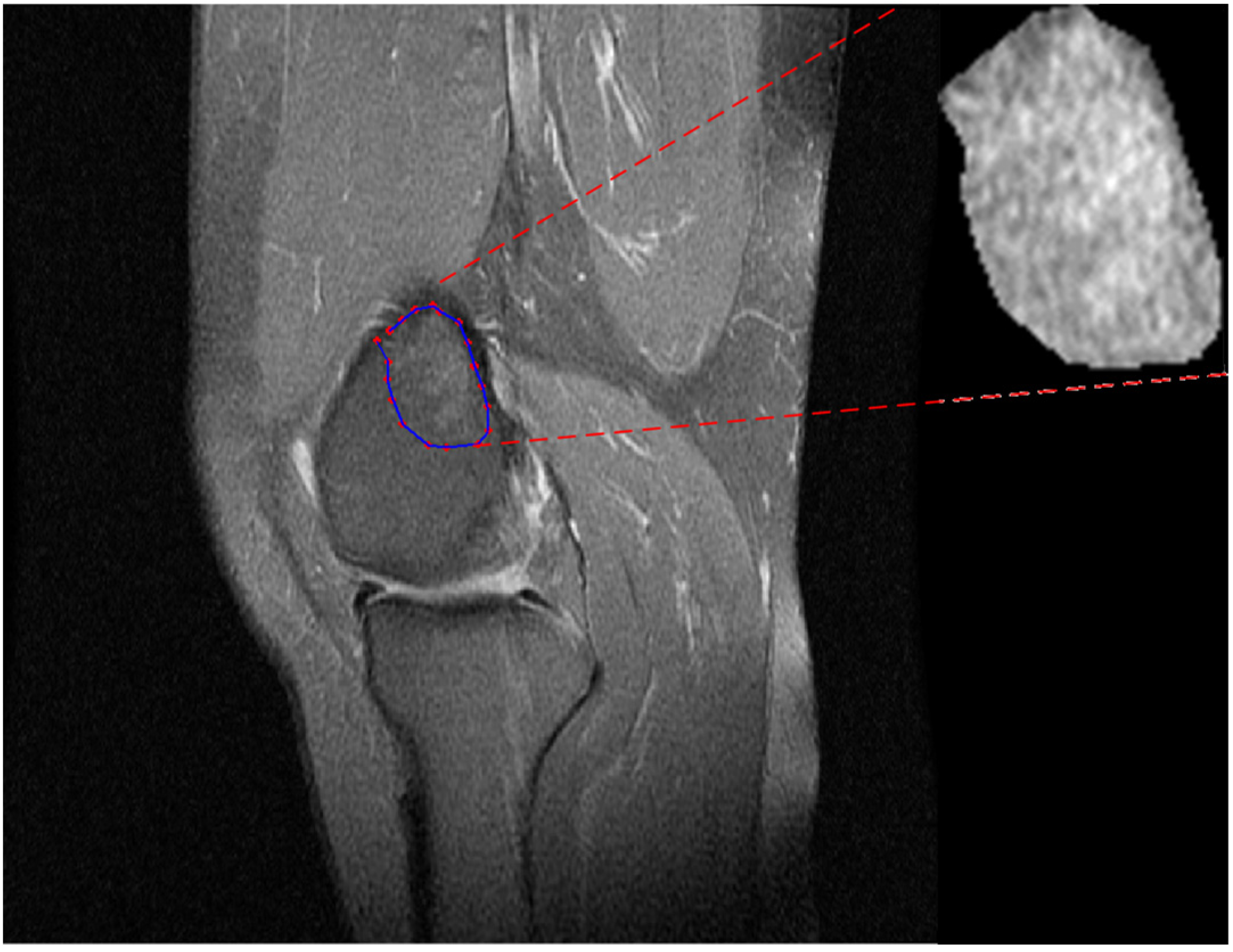
2.2. MRI Imaging Techniques and ROIs Delineation
2.3. Extraction of Radiomic Descriptors
- Twenty-two (22) of these were calculated based on the gray-level co-occurrence matrix (GLCM) [22,23,24,25,26] (angular second moment, contrast, correlation, sum of squares, inverse difference moment, sum average, sum variance, sum entropy, entropy, difference variance, difference entropy, information measure correlation 1, information measure correlation 2, maximal correlation coefficient, joint maximum, joint average, difference average, inverse difference, normalized inverse difference, autocorrelation, cluster shade, and cluster prominence).
- Sixteen (16) were computed based on the gray-level run-length matrix (GLRLM) [22,27,28,29,30] (short-run emphasis, long-run emphasis, gray-level non-uniformity, run-length non-uniformity, run percentage, low-gray run emphasis, high-gray run emphasis, short-run low-gray emphasis, short-run high-gray emphasis, long-run low-gray emphasis, long-run high-gray emphasis, normalized gray-level non-uniformity, normalized run-length non-uniformity, gray-level run variance, and run-length variance, run entropy). For GLCM and GLRLM descriptors, the average across four orientations (N, S, E, W) was determined (using 1 pixel offset).
- Sixteen (16) were considered based on the gray-level size zone matrix (GLSZM) [22,31] (small-zone emphasis, large-zone emphasis, low-gray-level zone emphasis, high-gray-level zone emphasis, small-zone low-grey emphasis, small-zone high-grey emphasis, large-zone low-grey emphasis, large-zone high-grey emphasis, gray-level non-uniformity, normalized gray-level non-uniformity, zone-size non-uniformity, normalized zone-size non-uniformity, zone percentage, grey-level zone variance, zone-size variance, zone-size entropy)
2.4. Statistical and Discriminant Analysis
3. Results and Discussion
4. Conclusions
Author Contributions
Funding
Institutional Review Board Statement
Informed Consent Statement
Data Availability Statement
Conflicts of Interest
References
- Beckwee, D.; Vaes, P.; Shahabpour, M.; Muyldermans, R.; Rommers, N.; Bautmans, I. The Influence of Joint Loading on Bone Marrow Lesions in the Knee: A Systematic Review With Meta-analysis. Am. J. Sports Med. 2015, 43, 3093–3107. [Google Scholar] [CrossRef] [PubMed]
- Hunter, D.J.; Gerstenfeld, L.; Bishop, G.; Davis, A.D.; Mason, Z.D.; Einhorn, T.A.; Maciewicz, R.A.; Newham, P.; Foster, M.; Jackson, S.; et al. Bone marrow lesions from osteoarthritis knees are characterized by sclerotic bone that is less well mineralized. Arthritis Res. Ther. 2009, 11, R11. [Google Scholar] [CrossRef] [PubMed]
- Zanetti, M.; Bruder, E.; Romero, J.; Hodler, J. Bone marrow edema pattern in osteoarthritic knees: Correlation between MR imaging and histologic findings. Radiology 2000, 215, 835–840. [Google Scholar] [CrossRef] [PubMed]
- Felson, D.T.; Chaisson, C.E.; Hill, C.L.; Totterman, S.M.; Gale, M.E.; Skinner, K.M.; Kazis, L.; Gale, D.R. The association of bone marrow lesions with pain in knee osteoarthritis. Ann. Intern. Med. 2001, 134, 541–549. [Google Scholar] [CrossRef]
- Felson, D.T.; McLaughlin, S.; Goggins, J.; LaValley, M.P.; Gale, M.E.; Totterman, S.; Li, W.; Hill, C.; Gale, D. Bone marrow edema and its relation to progression of knee osteoarthritis. Ann. Intern. Med. 2003, 139, 330–336. [Google Scholar] [CrossRef]
- Sowers, M.F.; Hayes, C.; Jamadar, D.; Capul, D.; Lachance, L.; Jannausch, M.; Welch, G. Magnetic resonance-detected subchondral bone marrow and cartilage defect characteristics associated with pain and X-ray-defined knee osteoarthritis. Osteoarthr. Cartil. 2003, 11, 387–393. [Google Scholar] [CrossRef]
- McAlindon, T.E.; Watt, I.; McCrae, F.; Goddard, P.; Dieppe, P.A. Magnetic resonance imaging in osteoarthritis of the knee: Correlation with radiographic and scintigraphic findings. Ann. Rheum. Dis. 1991, 50, 14–19. [Google Scholar] [CrossRef]
- Shi, X.; Mai, Y.; Fang, X.; Wang, Z.; Xue, S.; Chen, H.; Dang, Q.; Wang, X.; Tang, S.A.; Ding, C.; et al. Bone marrow lesions in osteoarthritis: From basic science to clinical implications. Bone Rep. 2023, 18, 101667. [Google Scholar] [CrossRef]
- Costa-Paz, M.; Muscolo, D.L.; Ayerza, M.; Makino, A.; Aponte-Tinao, L. Magnetic resonance imaging follow-up study of bone bruises associated with anterior cruciate ligament ruptures. Arthrosc. J. Arthrosc. Relat. Surg. Off. Publ. Arthrosc. Assoc. N. Am. Int. Arthrosc. Assoc. 2001, 17, 445–449. [Google Scholar] [CrossRef]
- Bretlau, T.; Tuxoe, J.; Larsen, L.; Jorgensen, U.; Thomsen, H.S.; Lausten, G.S. Bone bruise in the acutely injured knee. Knee Surg. Sports Traumatol. Arthrosc. Off. J. ESSKA 2002, 10, 96–101. [Google Scholar] [CrossRef]
- Roemer, F.W.; Bohndorf, K. Long-term osseous sequelae after acute trauma of the knee joint evaluated by MRI. Skelet. Radiol. 2002, 31, 615–623. [Google Scholar]
- Palmer, W.E.; Levine, S.M.; Dupuy, D.E. Knee and shoulder fractures: Association of fracture detection and marrow edema on MR images with mechanism of injury. Radiology 1997, 204, 395–401. [Google Scholar] [CrossRef] [PubMed]
- Adams, J.G.; McAlindon, T.; Dimasi, M.; Carey, J.; Eustace, S. Contribution of meniscal extrusion and cartilage loss to joint space narrowing in osteoarthritis. Clin. Radiol. 1999, 54, 502–506. [Google Scholar] [CrossRef] [PubMed]
- Li, X.; Ma, B.C.; Bolbos, R.I.; Stahl, R.; Lozano, J.; Zuo, J.; Lin, K.; Link, T.M.; Safran, M.; Majumdar, S. Quantitative assessment of bone marrow edema-like lesion and overlying cartilage in knees with osteoarthritis and anterior cruciate ligament tear using MR imaging and spectroscopic imaging at 3 Tesla. J. Magn. Reson. Imaging JMRI 2008, 28, 453–461. [Google Scholar] [CrossRef] [PubMed]
- Fritz, B.; Muller, D.A.; Sutter, R.; Wurnig, M.C.; Wagner, M.W.; Pfirrmann, C.W.A.; Fischer, M.A. Magnetic Resonance Imaging-Based Grading of Cartilaginous Bone Tumors: Added Value of Quantitative Texture Analysis. Investig. Radiol. 2018, 53, 663–672. [Google Scholar] [CrossRef]
- Cilengir, A.H.; Evrimler, S.; Serel, T.A.; Uluc, E.; Tosun, O. The diagnostic value of magnetic resonance imaging-based texture analysis in differentiating enchondroma and chondrosarcoma. Skelet. Radiol. 2023, 52, 1039–1049. [Google Scholar] [CrossRef]
- Chuah, T.K.; Van Reeth, E.; Sheah, K.; Poh, C.L. Texture analysis of bone marrow in knee MRI for classification of subjects with bone marrow lesion—Data from the Osteoarthritis Initiative. Magn. Reson. Imaging 2013, 31, 930–938. [Google Scholar] [CrossRef]
- MacKay, J.W.; Murray, P.J.; Low, S.B.L.; Kasmai, B.; Johnson, G.; Donell, S.T.; Toms, A.P. Quantitative analysis of tibial subchondral bone: Texture analysis outperforms conventional trabecular microarchitecture analysis. J. Magn. Reson. Imaging 2016, 43, 1159–1170. [Google Scholar] [CrossRef]
- Li, J.; Fu, S.; Gong, Z.; Zhu, Z.; Zeng, D.; Cao, P.; Lin, T.; Chen, T.; Wang, X.; Lartey, R.; et al. MRI-based Texture Analysis of Infrapatellar Fat Pad to Predict Knee Osteoarthritis Incidence. Radiology 2022, 304, 611–621. [Google Scholar] [CrossRef]
- Rizzo, S.; Botta, F.; Raimondi, S.; Origgi, D.; Fanciullo, C.; Morganti, A.G.; Bellomi, M. Radiomics: The facts and the challenges of image analysis. Eur. Radiol. Exp. 2018, 2, 36. [Google Scholar] [CrossRef]
- Kornaat, P.R.; Ceulemans, R.Y.; Kroon, H.M.; Riyazi, N.; Kloppenburg, M.; Carter, W.O.; Woodworth, T.G.; Bloem, J.L. MRI assessment of knee osteoarthritis: Knee Osteoarthritis Scoring System (KOSS)—Inter-observer and intra-observer reproducibility of a compartment-based scoring system. Skelet. Radiol. 2005, 34, 95–102. [Google Scholar] [CrossRef] [PubMed]
- Zwanenburg, A.; Leger, S.; Vallières, M.; Löck, S. Image biomarker standardisation initiative. arXiv 2016, arXiv:1612.07003. [Google Scholar]
- Haralick, R.; Shanmugam, K.; Dinstein, I. Textural features for image classification. IEEE Trans. Syst. Man Cybern. 1973, 3, 610–621. [Google Scholar] [CrossRef]
- Unser, M. Sum and difference histograms for texture classification. IEEE Trans. Pattern Anal. Mach. Intell. 1986, 8, 118–125. [Google Scholar] [CrossRef]
- Clausi, D.A. An analysis of co-occurrence texture statistics as a function of grey level quantization. Can. J. Remote Sens. 2002, 28, 45–62. [Google Scholar] [CrossRef]
- van Griethuysen, J.J.M.; Fedorov, A.; Parmar, C.; Hosny, A.; Aucoin, N.; Narayan, V.; Beets-Tan, R.G.H.; Fillion-Robin, J.C.; Pieper, S.; Aerts, H. Computational Radiomics System to Decode the Radiographic Phenotype. Cancer Res. 2017, 77, e104–e107. [Google Scholar] [CrossRef]
- Galloway, M.M. Texture Analysis Using Grey Level Run Lengths. Comput. Graph. Image Process. 1975, 4, 172–179. [Google Scholar] [CrossRef]
- Chu, A.; Sehgal, C.M.; Greenleaf, J.F. Use of gray value distribution of run lengths for texture analysis. Pattern Recognit. Lett. 1990, 11, 415–419. [Google Scholar] [CrossRef]
- Dasarathy, B.V.; Holder, E.B. Image characterizations based on joint gray level—Run length distributions. Pattern Recognit. Lett. 1991, 12, 497–502. [Google Scholar] [CrossRef]
- Albregtsen, F.; Nielsen, B.; Danielsen, H.E. Adaptive gray level run length features from class distance matrices. In Proceedings of the 15th International Conference on Pattern Recognition, ICPR-2000, Barcelona, Spain, 3–7 September 2000; Volume 733, pp. 738–741. [Google Scholar]
- Thibault, G.; Angulo, J.; Meyer, F. Advanced Statistical Matrices for Texture Characterization: Application to Cell Classification. IEEE Trans. Biomed. Eng. 2014, 61, 630–637. [Google Scholar] [CrossRef]
- Tamura, H.; Mori, S.; Yamawaki, T. Textural Features Corresponding to Visual Perception. IEEE Trans. Syst. Man Cybern. 1978, SMC-8, 460–472. [Google Scholar] [CrossRef]
- El Merabet, Y.; Ruichek, Y.; El Idrissi, A. Attractive-and-repulsive center-symmetric local binary patterns for texture classification. Eng. Appl. Artif. Intell. 2019, 78, 158–172. [Google Scholar] [CrossRef]
- Jarque, C.M.; Bera, A.K. A Test for Normality of Observations and Regression Residuals. Int. Stat. Rev. Rev. Int. De Stat. 1987, 55, 163–172. [Google Scholar] [CrossRef]
- McKight, P.E.; Najab, J. Kruskal-Wallis Test. In The Corsini Encyclopedia of Psychology; John Wiley & Sons: New York, NY, USA, 2010; p. 1. [Google Scholar]
- Hochberg, Y.; Tamhane, A.C. Multiple Comparison Procedures; John Wiley & Sons: Hoboken, NJ, USA, 1987. [Google Scholar]
- Storey, J.D. A direct approach to false discovery rates. J. R. Stat. Soc. Ser. B 2002, 64, 479–498. [Google Scholar] [CrossRef]
- Benjamini, Y.; Hochberg, Y. Controlling the False Discovery Rate: A Practical and Powerful Approach to Multiple Testing. J. R. Stat. Soc. Ser. B 1995, 57, 289–300. [Google Scholar] [CrossRef]
- Pedregosa, F.; Varoquaux, G.; Gramfort, A.; Michel, V.; Thirion, B.; Grisel, O.; Blondel, M.; Prettenhofer, P.; Weiss, R.; Dubourg, V.; et al. Scikit-learn: Machine Learning in Python. J. Mach. Learn. Res. 2011, 12, 2825–2830. [Google Scholar]
- Wehrli, F.W. Structural and functional assessment of trabecular and cortical bone by micro magnetic resonance imaging. J. Magn. Reson. Imaging 2007, 25, 390–409. [Google Scholar] [CrossRef]
- Hu, Y.; Chen, X.; Wang, S.; Jing, Y.; Su, J. Subchondral bone microenvironment in osteoarthritis and pain. Bone Res. 2021, 9, 20. [Google Scholar] [CrossRef]
- Pop, T.S.; Miron, A.D.T.; Pop, A.M.; Brinzaniuc, K.; Trambitas, C. Magnetic Resonance Imaging Assessment of Bone Regeneration in Osseous Defects Filled with Different Biomaterials. An experimental in vivo study. Mater. Plast. 2019, 56, 235–238. [Google Scholar] [CrossRef]
- Kühn, J.P.; Hernando, D.; Meffert, P.J.; Reeder, S.; Hosten, N.; Laqua, R.; Steveling, A.; Ender, S.; Schröder, H.; Pillich, D.T. Proton-density fat fraction and simultaneous R2* estimation as an MRI tool for assessment of osteoporosis. Eur. Radiol. 2013, 23, 3432–3439. [Google Scholar] [CrossRef]


| Sequences | PD-FSE | STIR |
|---|---|---|
| Parameters | ||
| ΤR (ms) | 2200 | 5675 |
| TE (ms) | 30 | 50 |
| ETL | 8 | 16 |
| Band Width (kHz) | 31.25 | 20.83 |
| Freq | 384 × 224 | 256 × 192 |
| Freq DIR | A/P | A/P |
| Slice Thickness (mm) | 4.0 | 4.0 |
| Spacing (mm) | 0.8 | 0.8 |
| FOV (mm) | 18 | 18 |
| Slices | 19 | 18 |
| Acquisition Time (min) | 2′.17″ | 2′.22″ |
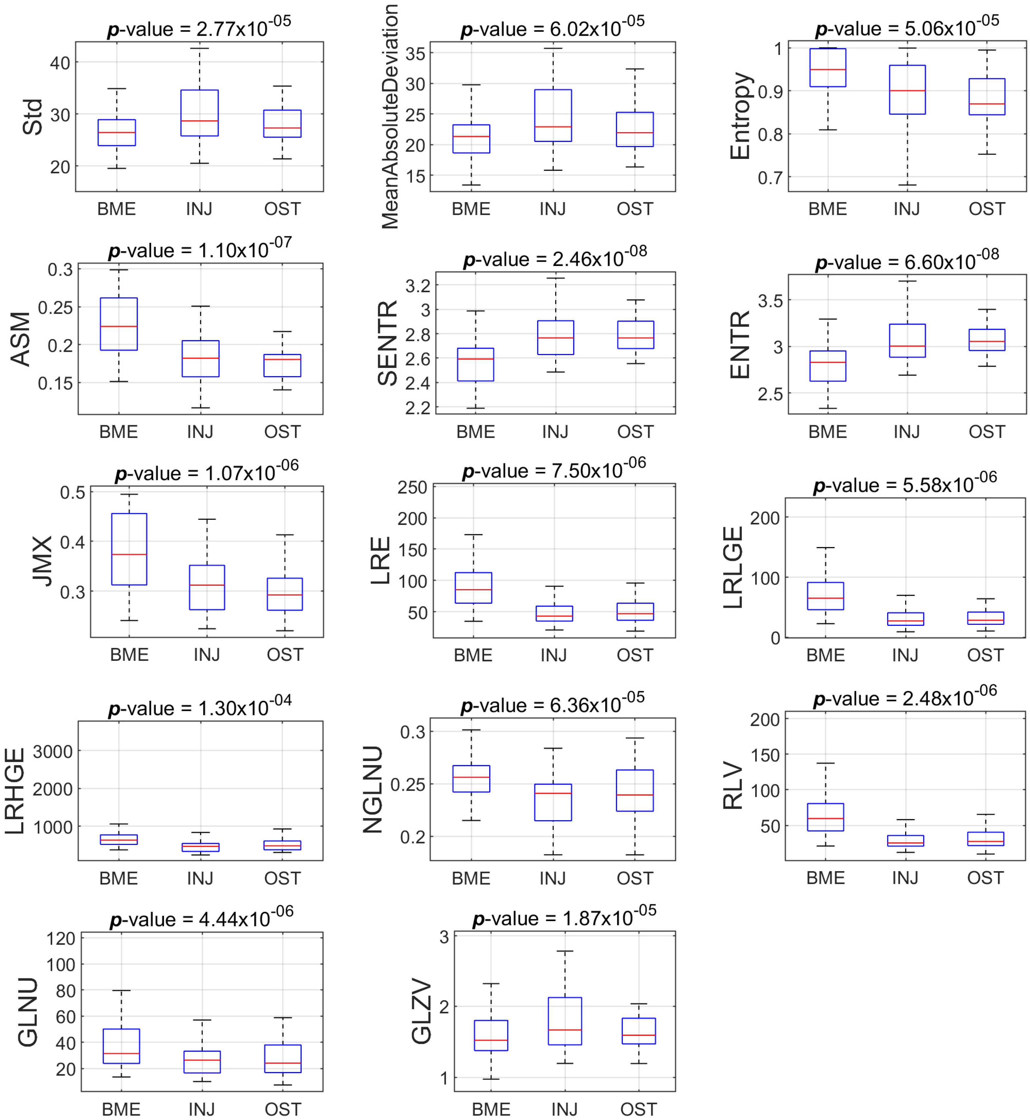
| Feature | BME Mean ± Std or Median (IQR) | INJ Mean ± Std or Median (IQR) | OST Mean ± Std or Median (IQR) | Description of Post Hoc Pairwise Comparison (p < 0.001) |
|---|---|---|---|---|
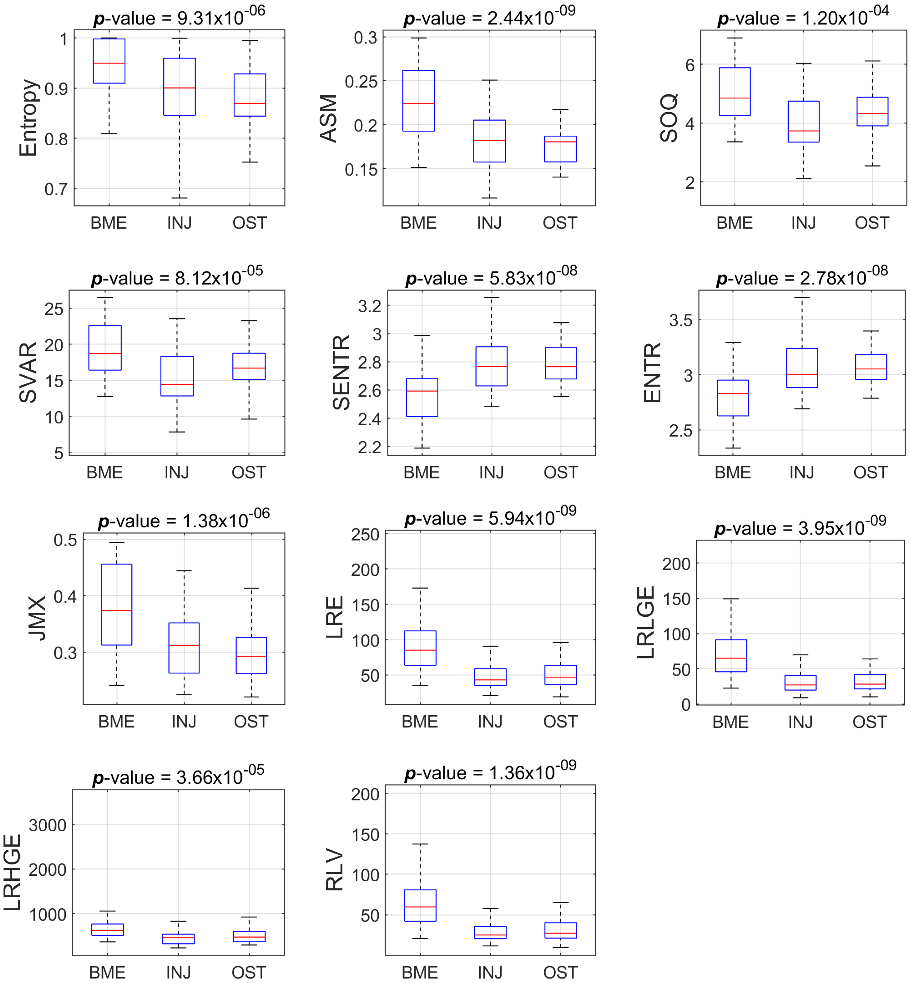
| Entropy | 0.95 (0.09) | 0.90 (0.11) | 0.87 (0.08) | The mean ranks of groups BME and OST are significantly different |
| ASM | 0.22 (0.07) | 0.18 (0.05) | 0.18 (0.03) | Two groups have mean ranks significantly different from BME |
| SOQ | 4.86 (1.63) | 3.74 (1.39) | 4.32 (0.97) | The mean ranks of groups BME and INJ are significantly different |
| SVAR | 18.73 (6.17) | 14.45 (5.48) | 16.71 (3.65) | The mean ranks of groups BME and INJ are significantly different |
| SENTR | 2.59 (0.27) | 2.77 (0.28) | 2.77 (0.22) | Two groups have mean ranks significantly different from BME |
| ENTR | 2.83( 0.32) | 3.00 (0.35) | 3.05 (0.23) | Two groups have mean ranks significantly different from BME |
| JMX | 0.38± 0.08 | 0.32± 0.06 | 0.30± 0.05 | The mean ranks of groups BME and OST are significantly different |
| LRE | 97.74 ± 49.12 | 53.51 ± 29.61 | 51.62 ± 19.99 | Two groups have mean ranks significantly different from BME |
| LRLGE | 77.56 ± 47.40 | 36.40 ± 25.90 | 33.93 ± 17.51 | Two groups have mean ranks significantly different from BME |
| LRHGE | 727.09 ± 497.94 | 478.65 ± 179.35 | 553.00 ± 229.49 | The mean ranks of groups BME and INJ are significantly different |
| RLV | 70.55 ± 41.60 | 33.38 ± 21.96 | 32.01 ± 14.96 | Two groups have mean ranks significantly different from BME |
| Feature | BME Mean ± Std or Median (IQR) | INJ Mean ± Std or Median (IQR) | OST Mean ± Std or Median (IQR) | Description of Post Hoc Pairwise Comparison (p < 0.001) |
|---|---|---|---|---|
| Std | 29.10 (7.87) | 36.58 (8.57) | 33.29 (7.71) | Two groups have means significantly different from BME |
| MAD | 23.64 (6.66) | 29.40 (8.18) | 27.09 (6.30) | Two groups have means significantly different from BME |
| Entropy | 0.96± 0.05 | 0.90± 0.07 | 0.92± 0.06 | The mean ranks of groups BME and INJ are significantly different |
| ASM | 0.20± 0.05 | 0.15± 0.03 | 0.15 ± 0.04 | Two groups have mean ranks significantly different from BME |
| SENTR | 2.72 ± 0.23 | 3.02 ± 0.18 | 3.00 ± 0.23 | Two groups have mean ranks significantly different from BME |
| ENTR | 3.12 ± 0.30 | 3.50 ± 0.25 | 3.47 ± 0.32 | Two groups have mean ranks significantly different from BME |
| JMX | 0.37 ± 0.08 | 0.28 ± 0.06 | 0.30 ± 0.06 | Two groups have mean ranks significantly different from BME |
| LRE | 43.60 ± 26.98 | 22.57 ± 12.06 | 25.47 ± 16.69 | Two groups have mean ranks significantly different from BME |
| LRLGE | 33.96 ± 24.88 | 14.74 ± 10.28 | 17.26 ± 12.92 | Two groups have mean ranks significantly different from BME |
| LRHGE | 277.32 ± 122.49 | 195.16 ± 80.30 | 217.82 ± 132.22 | The mean ranks of groups BME and INJ are significantly different |
| NGLNU | 0.23 ± 0.02 | 0.21 ± 0.02 | 0.22 ± 0.02 | Two groups have mean ranks significantly different from BME |
| RLV | 29.22 ± 20.74 | 12.80 ± 8.49 | 14.52 ± 10.82 | Two groups have mean ranks significantly different from BME |
| GLNUsz | 21.48 ± 10.27 | 14.00 ± 8.35 | 12.23 ± 5.76 | Two groups have mean ranks significantly different from BME |
| GLZV | 1.7 4 0.50) | 2.27 (0.54) | 2.08 (0.51) | The means of groups BME and INJ are significantly different |
| k-fold | Acc | TPR | AUC | ||
|---|---|---|---|---|---|
| BME | INJ | OST | |||
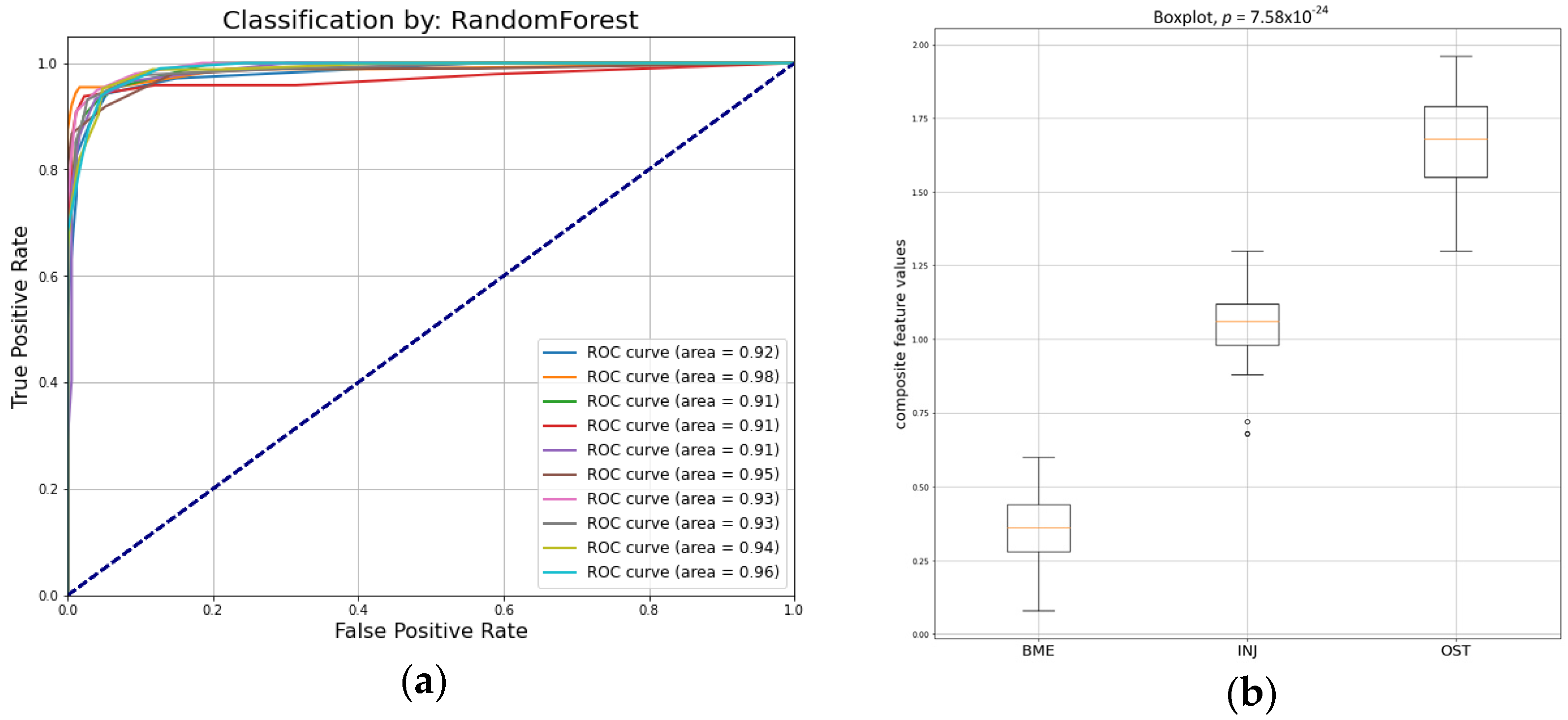
| 1 | 0.89 | 0.89 | 0.89 | 0.89 | 0.92 |
| 2 | 0.96 | 0.99 | 0.94 | 0.94 | 0.98 |
| 3 | 0.91 | 0.93 | 0.90 | 0.91 | 0.91 |
| 4 | 0.92 | 0.90 | 0.90 | 0.96 | 0.91 |
| 5 | 0.91 | 0.91 | 0.93 | 0.89 | 0.91 |
| 6 | 0.92 | 0.94 | 0.87 | 0.95 | 0.95 |
| 7 | 0.93 | 0.94 | 0.92 | 0.93 | 0.93 |
| 8 | 0.93 | 0.93 | 0.91 | 0.94 | 0.93 |
| 9 | 0.91 | 0.98 | 0.90 | 0.86 | 0.94 |
| 10 | 0.93 | 0.96 | 0.92 | 0.91 | 0.96 |
| Average (std) | 0.92 (0.02) | 0.94 (0.03) | 0.91 (0.02) | 0.92 (0.03) | 0.93 (0.02) |
Disclaimer/Publisher’s Note: The statements, opinions and data contained in all publications are solely those of the individual author(s) and contributor(s) and not of MDPI and/or the editor(s). MDPI and/or the editor(s) disclaim responsibility for any injury to people or property resulting from any ideas, methods, instructions or products referred to in the content. |
© 2023 by the authors. Licensee MDPI, Basel, Switzerland. This article is an open access article distributed under the terms and conditions of the Creative Commons Attribution (CC BY) license (https://creativecommons.org/licenses/by/4.0/).
Share and Cite
Kostopoulos, S.; Boci, N.; Cavouras, D.; Tsagkalis, A.; Papaioannou, M.; Tsikrika, A.; Glotsos, D.; Asvestas, P.; Lavdas, E. Radiomics Texture Analysis of Bone Marrow Alterations in MRI Knee Examinations. J. Imaging 2023, 9, 252. https://doi.org/10.3390/jimaging9110252
Kostopoulos S, Boci N, Cavouras D, Tsagkalis A, Papaioannou M, Tsikrika A, Glotsos D, Asvestas P, Lavdas E. Radiomics Texture Analysis of Bone Marrow Alterations in MRI Knee Examinations. Journal of Imaging. 2023; 9(11):252. https://doi.org/10.3390/jimaging9110252
Chicago/Turabian StyleKostopoulos, Spiros, Nada Boci, Dionisis Cavouras, Antonios Tsagkalis, Maria Papaioannou, Alexandra Tsikrika, Dimitris Glotsos, Pantelis Asvestas, and Eleftherios Lavdas. 2023. "Radiomics Texture Analysis of Bone Marrow Alterations in MRI Knee Examinations" Journal of Imaging 9, no. 11: 252. https://doi.org/10.3390/jimaging9110252
APA StyleKostopoulos, S., Boci, N., Cavouras, D., Tsagkalis, A., Papaioannou, M., Tsikrika, A., Glotsos, D., Asvestas, P., & Lavdas, E. (2023). Radiomics Texture Analysis of Bone Marrow Alterations in MRI Knee Examinations. Journal of Imaging, 9(11), 252. https://doi.org/10.3390/jimaging9110252