
3D Dynamic Spatiotemporal Atlas of the Vocal Tract during Consonant–Vowel Production from 2D Real Time MRI

 ,
,
Abstract
:1. Introduction
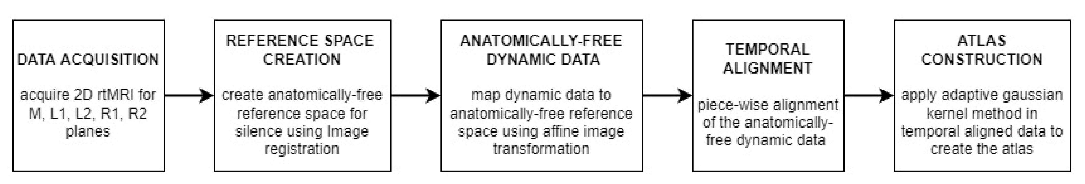
2. Method
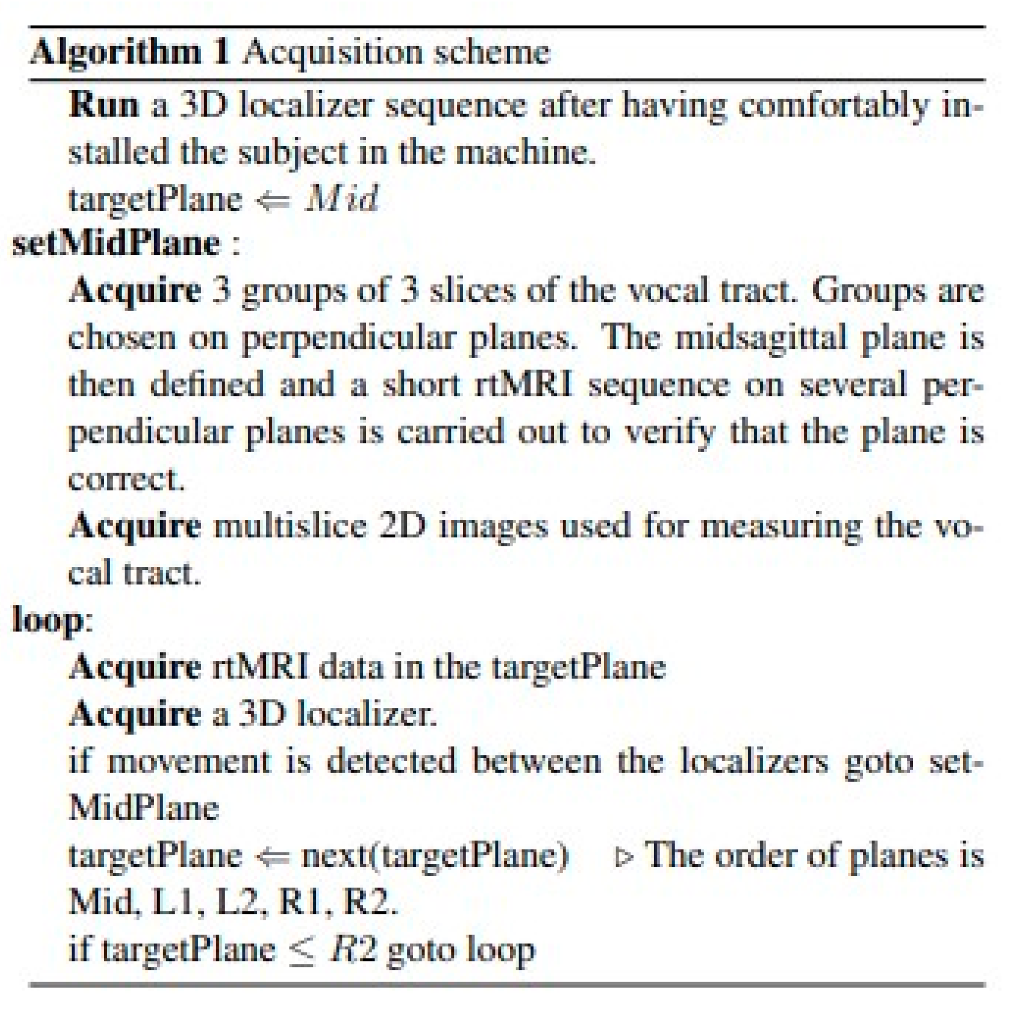
- (1)
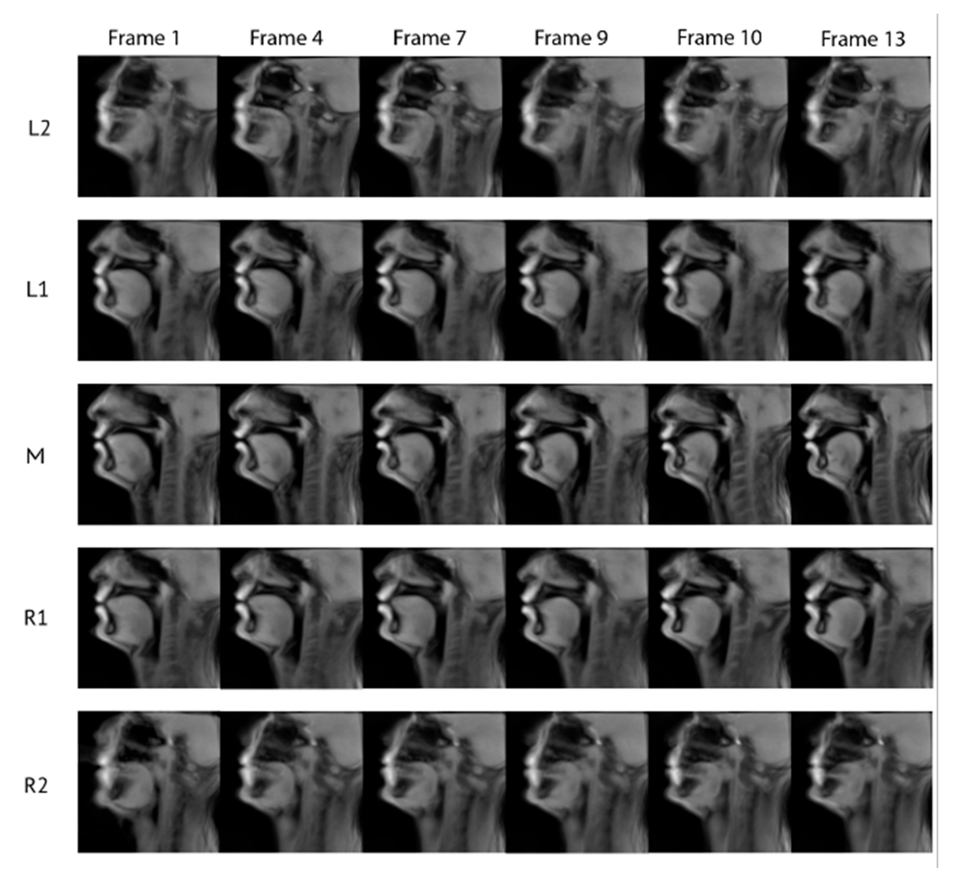
- Acquire 2D dynamic rtMRI parallel sagittal planes of the vocal tract during the production of several CVs;
- (2)
- Create a subject-independent anatomical space based on a silent articulatory configuration;
- (3)
- Use this space to remove the subject’s specific anatomical information from the dynamic images;
- (4)
- Combine the previously created “anatomical neutral” dynamic images using piece-wise alignment and adaptive Gaussian kernel to create the dynamic atlas.
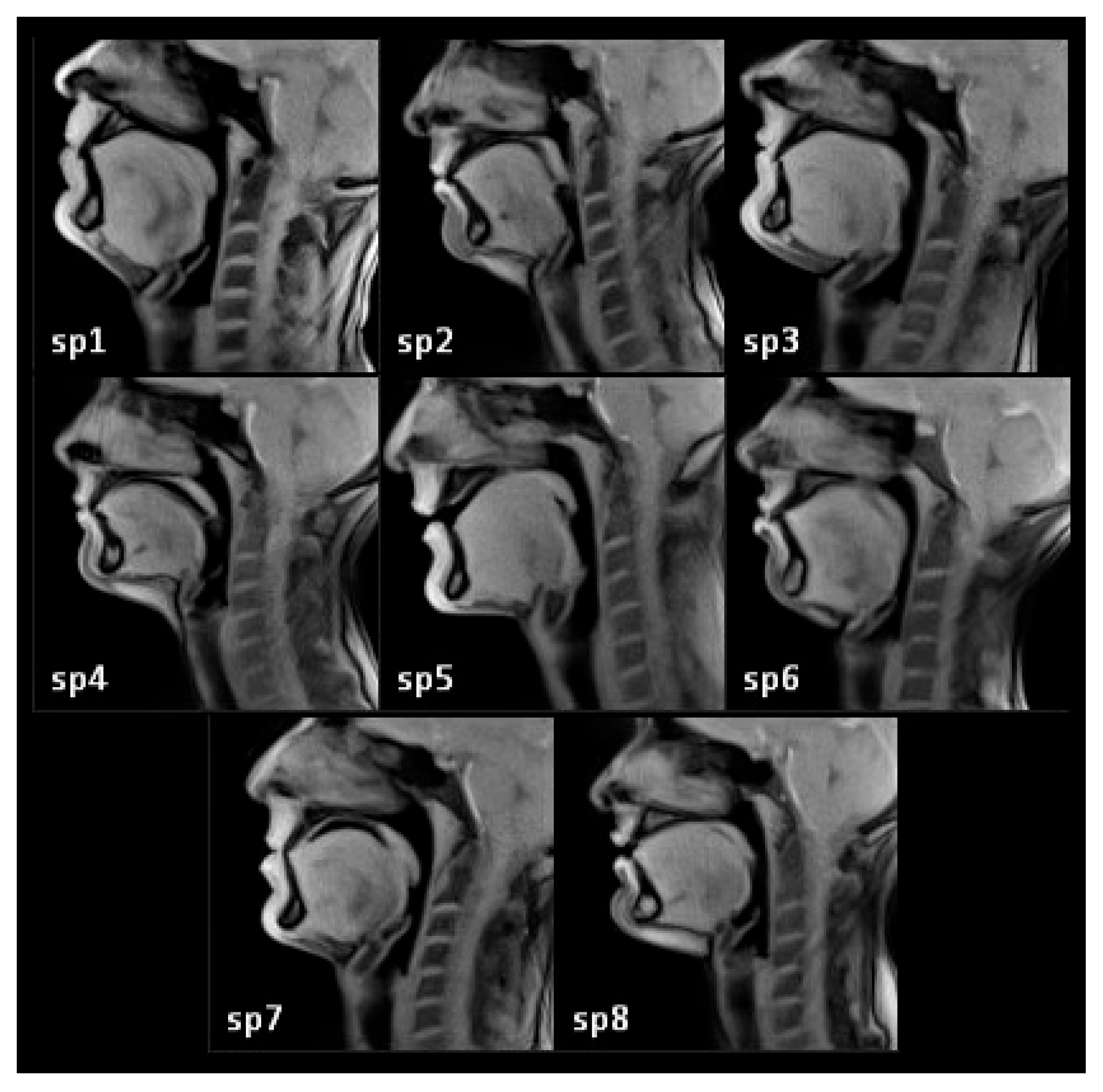
2.1. Subjects
2.2. Data Acquisition
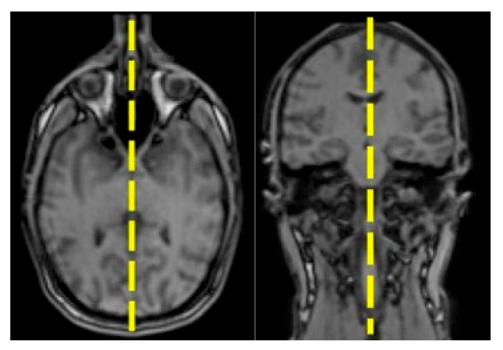
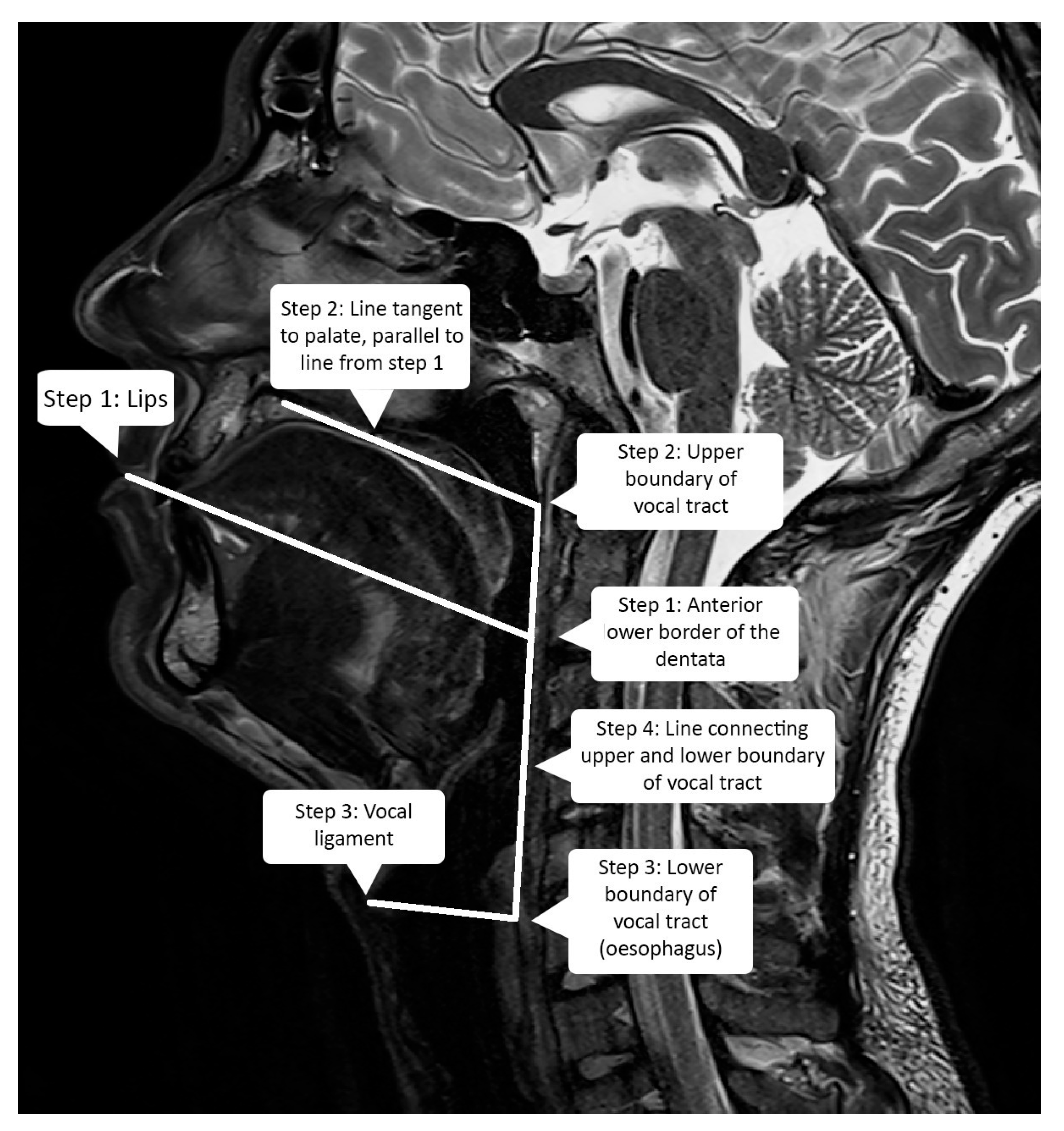
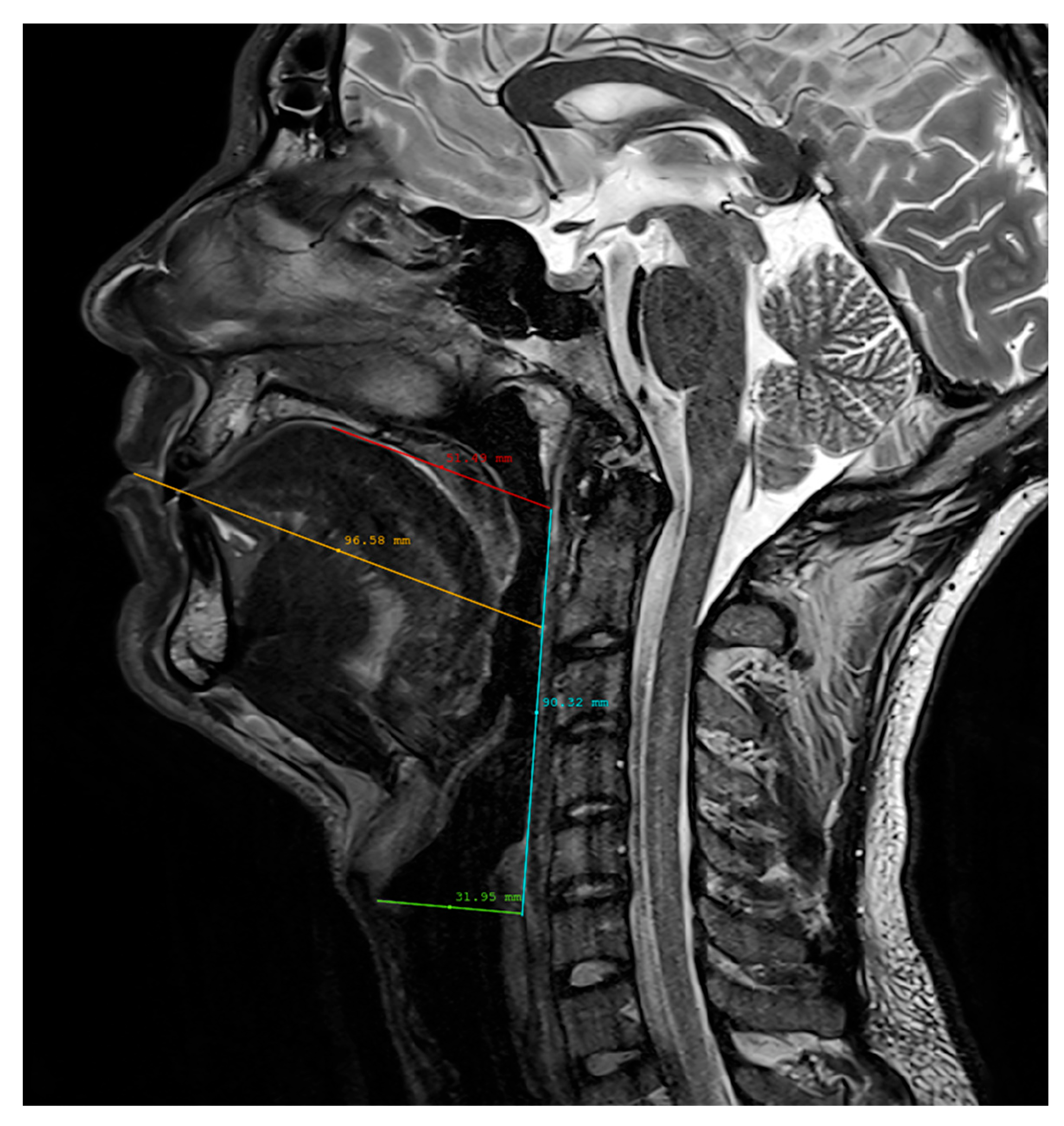
2.3. Vocal Tract Measurements
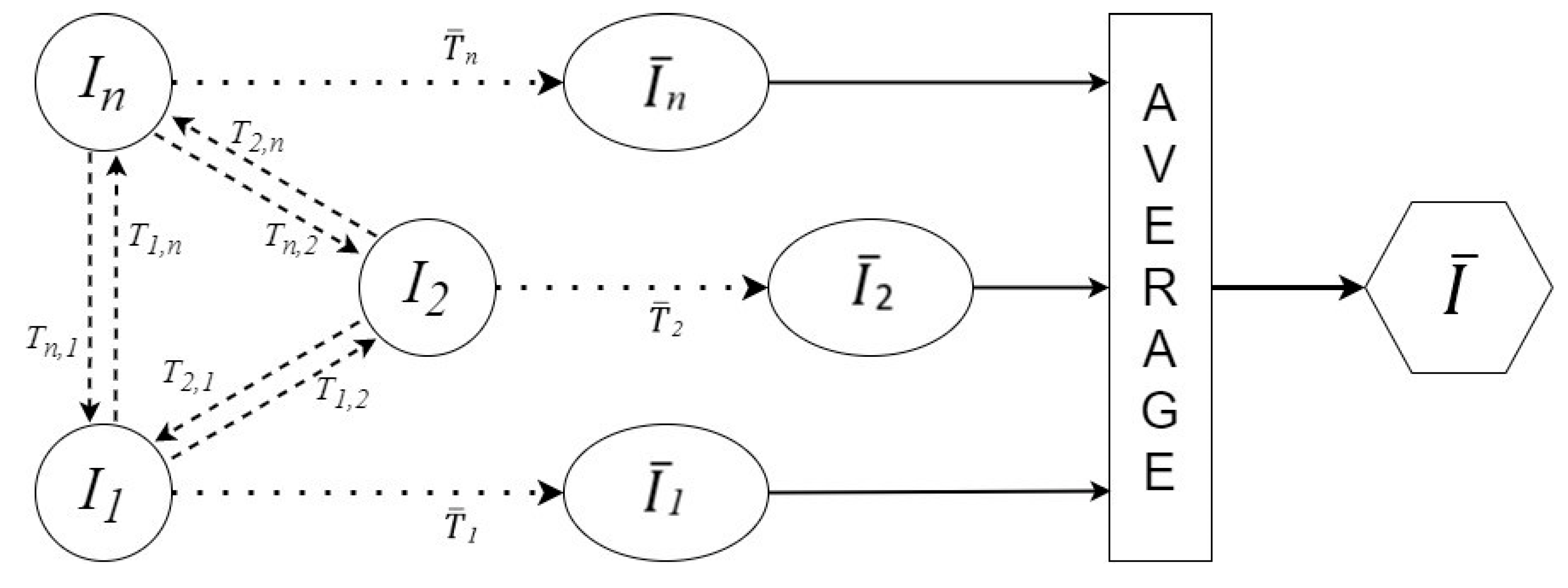
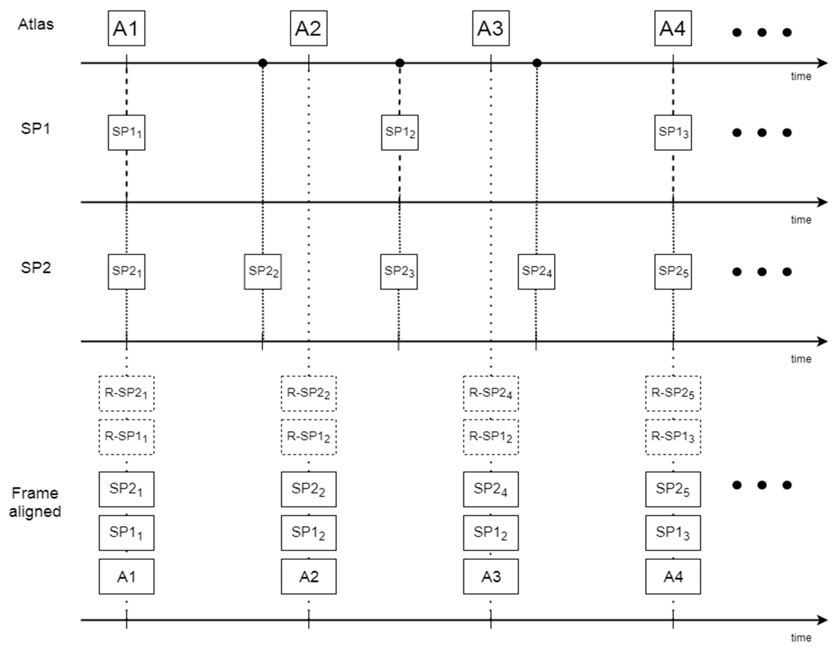
2.4. Atlas Construction
- (1)
- Create the anatomically free reference space;
- (2)
- Make dynamic data anatomically free;
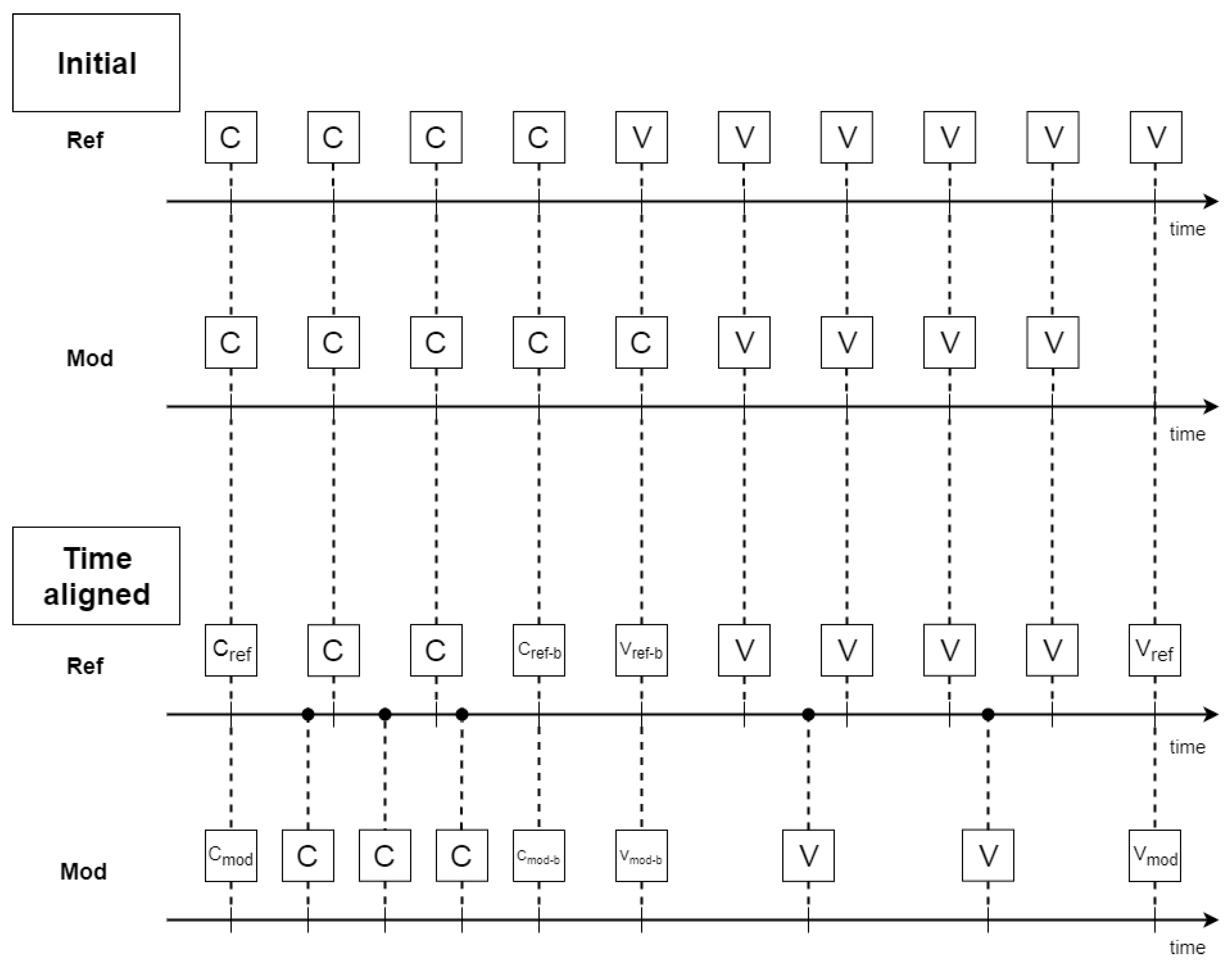
- (3)
- Align data temporarily;
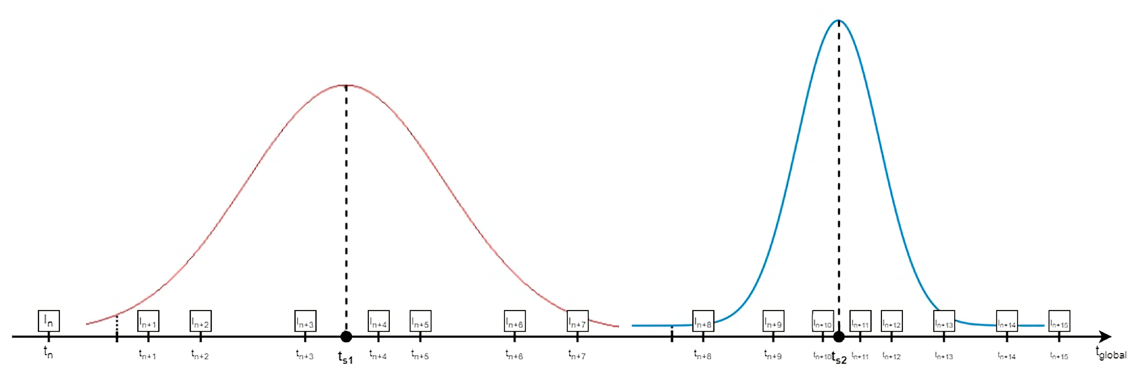
- (4)
- Synthesize the atlas samples.
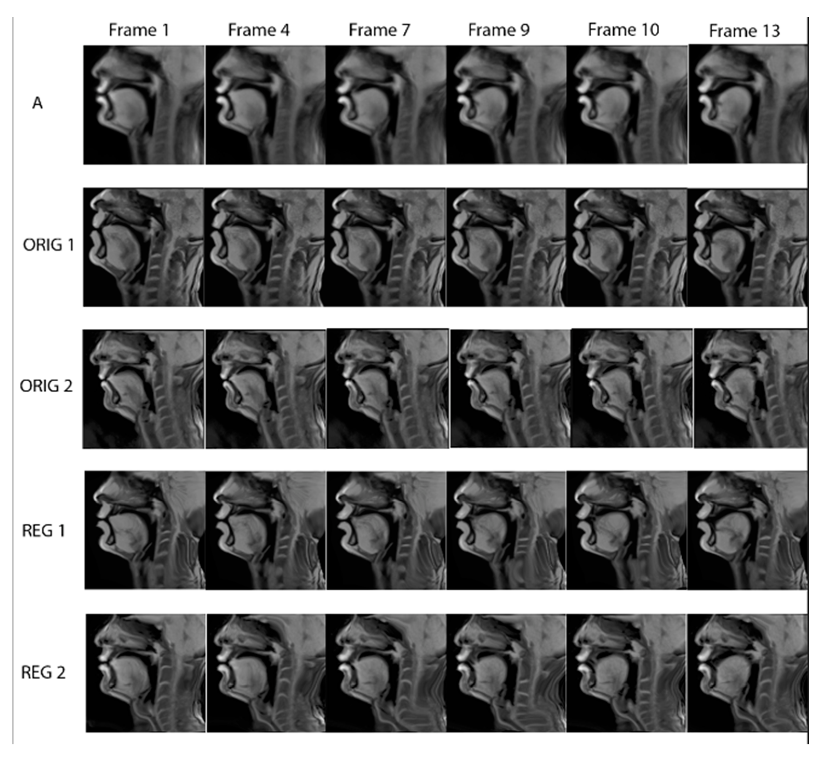
3. Validation
4. Results
5. Discussion
6. Conclusions
Author Contributions
Funding
Institutional Review Board Statement
Informed Consent Statement
Acknowledgments
Conflicts of Interest
References
- Gousias, I.S.; Rueckert, D.; Heckemann, R.A.; Dyet, L.E.; Boardman, J.P.; Edwards, A.D.; Hammers, A. Automatic segmentation of brain MRIs of 2-year-olds into 83 regions of interest. Neuroimage 2008, 40, 672–684. [Google Scholar] [CrossRef] [PubMed]
- Seghers, D.; D’Agostino, E.; Maes, F.; Vandermeulen, D.; Suetens, P. Construction of a brain template from mr images using state-of-the-art registration and segmentation techniques. In Proceedings of the International Conference on Medical Image Computing and Computer-Assisted Intervention, Saint-Malo, France, 26–29 September 2004; Springer: Berlin/Heidelberg, Germany, 2004; pp. 696–703. [Google Scholar]
- Ericsson, A.; Aljabar, P.; Rueckert, D. Construction of a patient-specific atlas of the brain: Application to normal aging. In Proceedings of the 2008 5th IEEE International Symposium on Biomedical Imaging: From Nano to Macro, Paris, France, 14–17 May 2008; pp. 480–483. [Google Scholar]
- Agarwal, N.; Xu, X.; Gopi, M. Robust registration of mouse brain slices with severe histological artifacts. In Proceedings of the Tenth Indian Conference on Computer Vision, Graphics and Image Processing, Guwahati, India, 18–22 December 2016; ACM: New York, NY, USA, 2016; p. 10. [Google Scholar]
- Xiong, J.; Ren, J.; Luo, L.; Horowitz, M. Mapping histological slice sequences to the allen mouse brain atlas without 3d reconstruction. Front. Neuroinformatics 2018, 12, 93. [Google Scholar] [CrossRef] [PubMed]
- Chuang, N.; Mori, S.; Yamamoto, A.; Jiang, H.; Ye, X.; Xu, X.; Richards, L.J.; Nathans, J.; Miller, M.I.; Toga, A.W.; et al. An mri-based atlas and database of the developing mouse brain. Neuroimage 2011, 54, 80–89. [Google Scholar] [CrossRef] [PubMed]
- Calabrese, E.; Badea, A.; Watson, C.; Johnson, G.A. A quantitative magnetic resonance histology atlas of postnatal rat brain development with regional estimates of growth and variability. Neuroimage 2013, 71, 196–206. [Google Scholar] [CrossRef]
- Davis, B.C.; Fletcher, P.T.; Bullitt, E.; Joshi, S. Population shape regression from random design data. Int. J. Comput. Vis. 2010, 90, 255–266. [Google Scholar] [CrossRef]
- Liao, S.; Jia, H.; Wu, G.; Shen, D. Alzheimer’s Disease Neuroimaging Initiative. A novel framework for longitudinal atlas construction with groupwise registration of subject image sequences. NeuroImage 2012, 59, 1275–1289. [Google Scholar] [CrossRef]
- Kuklisova-Murgasova, M.; Aljabar, P.; Srinivasan, L.; Counsell, S.J.; Doria, V.; Serag, A.; Gousias, I.S.; Boardman, J.P.; Rutherford, M.A.; Edwards, A.D.; et al. A dynamic 4d probabilistic atlas of the developing brain. NeuroImage 2011, 54, 2750–2763. [Google Scholar] [CrossRef]
- Serag, A.; Aljabar, P.; Ball, G.; Counsell, S.J.; Boardman, J.P.; Rutherford, M.A.; Edwards, A.D.; Hajnal, J.V.; Rueckert, D. Construction of a consistent high-definition spatio-temporal atlas of the developing brain using adaptive kernel regression. Neuroimage 2012, 59, 2255–2265. [Google Scholar] [CrossRef]
- Takemoto, H. Morphological analyses of the human tongue musculature for three-dimensional modeling. J. Speech Lang. Hear. Res. 2001, 44, 95–107. [Google Scholar] [CrossRef]
- Stone, M.; Davis, E.P.; Douglas, A.S.; NessAiver, M.; Gullapalli, R.; Levine, W.S.; Lundberg, A. Modeling the motion of the internal tongue from tagged cine-images. J. Acoust. Soc. Am. 2001, 109, 2974–2982. [Google Scholar] [CrossRef] [Green Version]
- Parthasarathy, V.; Prince, J.L.; Stone, M.; Murano, E.Z.; NessAiver, M. Measuring tongue motion from tagged cine-mri using harmonic phase (harp) processing. J. Acoust. Soc. Am. 2007, 121, 491–504. [Google Scholar] [CrossRef]
- Xing, F.; Prince, J.L.; Stone, M.; Wedeen, V.J.; El Fakhri, G.; Woo, J. A four-dimensional motion field atlas of the tongue from tagged and cine magnetic resonance imaging. In Medical Imaging 2017: Image Processing; International Society for Optics and Photonics: Bellingham, WA, USA, 2017; Volume 10133, p. 101331H. [Google Scholar]
- Woo, J.; Xing, F.; Stone, M.; Green, J.; Reese, T.G.; Brady, T.J.; Wedeen, V.J.; Prince, J.L.; El Fakhri, G. Speech map: A statistical multimodal atlas of 4d tongue motion during speech from tagged and cine mr images. Comput. Methods Biomech. Biomed. Eng. Imaging Vis. 2019, 7, 361–373. [Google Scholar] [CrossRef]
- Xing, F.; Stone, M.; Goldsmith, T.; Prince, J.L.; El Fakhri, G.; Woo, J. Atlas-based tongue muscle correlation analysis from tagged and high- resolution magnetic resonance imaging. J. Speech Lang. Hear. Res. 2019, 62, 2258–2269. [Google Scholar] [CrossRef]
- Skordilis, Z.I.; Toutios, A.; Töger, J.; Narayanan, S. Estimation of vocal tract area function from volumetric magnetic resonance imaging. In Proceedings of the 2017 IEEE International Conference on Acoustics, Speech and Signal Processing (ICASSP), New Orleans, LA, USA, 5–9 March 2017; pp. 924–928. [Google Scholar]
- Takemoto, H.; Honda, K.; Masaki, S.; Shimada, Y.; Fujimoto, I. Measurement of temporal changes in vocal tract area function from 3d cine-MRIdata. J. Acoust. Soc. Am. 2006, 119, 1037–1049. [Google Scholar] [CrossRef]
- Fu, M.; Woo, J.; Liang, Z.-P.; Sutton, B.P. Spatiotemporal-atlas-based dynamic speech imaging. In Medical Imaging 2016: Biomedical Applications in Molecular, Structural, and Functional Imaging; International Society for Optics and Photonics: Bellingham, WA, USA, 2016; Volume 9788, p. 978804. [Google Scholar]
- Woo, J.; Lee, J.; Murano, E.Z.; Xing, F.; Al-Talib, M.; Stone, M.; Prince, J.L. A high-resolution atlas and statistical model of the vocal tract from structuralMRI. Comput. Methods Biomech. Biomed. Eng. Imaging Vis. 2015, 3, 47–60. [Google Scholar] [CrossRef]
- Woo, J.; Xing, F.; Lee, J.; Stone, M.; Prince, J.L. Construction of an unbiased spatio- temporal atlas of the tongue during speech. In Proceedings of the International Conference on Information Processing in Medical Imaging, Isle of Skye, UK, 28 June–3 July 2015; Springer: Berlin/Heidelberg, Germany, 2015; pp. 723–732. [Google Scholar]
- Woo, J.; Xing, F.; Lee, J.; Stone, M.; Prince, J.L. A spatio-temporal atlas and statistical model of the tongue during speech from cine-MRI. Comput. Methods Biomech. Biomed. Eng. Imaging Vis. 2018, 6, 520–531. [Google Scholar] [CrossRef]
- Ramanarayanan, V.; Tilsen, S.; Proctor, M.; Töger, J.; Goldstein, L.; Nayak, K.S.; Narayanan, S. Analysis of speech production real-time MRI. Comput. Speech Lang. 2018, 52, 1–22. [Google Scholar] [CrossRef]
- Maeda, S. Compensatory articulation during speech: Evidence from the analysis and synthesis of vocal-tract shapes using an articulatory model. In Speech Production and Speech Modelling; Springer: Berlin/Heidelberg, Germany, 1990; pp. 131–149. [Google Scholar]
- Lim, Y.; Zhu, Y.; Lingala, S.G.; Byrd, D.; Narayanan, S.; Nayak, K.S. 3d dynamic MRIof the vocal tract during natural speech. Magn. Reson. Med. 2019, 81, 1511–1520. [Google Scholar] [CrossRef]
- Zhao, Z.; Lim, Y.; Byrd, D.; Narayanan, S.; Nayak, K.S. Improved 3D real-time MRI of speech production. Magn. Reson. Med. 2020, 85, 3182–3195. [Google Scholar] [CrossRef]
- Uecker, M.; Zhang, S.; Voit, D.; Karaus, A.; Merboldt, K.-D.; Frahm, J. Real-time MRIat a resolution of 20 ms. NMR Biomed. 2010, 23, 986–994. [Google Scholar] [CrossRef] [Green Version]
- Niebergall, A.; Zhang, S.; Kunay, E.; Keydana, G.; Job, M.; Uecker, M.; Frahm, J. Real-Time MRI of Speaking at a Resolution of 33 ms: Undersampled Radial FLASH with Nonlinear Inverse Reconstruction. Magn. Reson. Med. 2013, 69, 477–485. [Google Scholar] [CrossRef] [PubMed]
- Roers, F.; Mürbe, D.; Sundberg, J. Voice classification and vocal tract of singers: A study of x-ray images and morphology. J. Acoust. Soc. Am. 2009, 125, 503–512. [Google Scholar] [CrossRef] [PubMed]
- Perry, J.L.; Kuehn, D.P.; Sutton, B.P.; Fang, X. Velopharyngeal structural and functional assessment of speech in young children using dynamic magnetic resonance imaging. Cleft Palate-Craniofacial J. 2017, 54, 408–422. [Google Scholar] [CrossRef] [PubMed]
- Eslami, M.; Neuschaefer-Rube, C.; Serrurier, A. Automatic vocal tract landmark localization from midsagittal MRIdata. Sci. Rep. 2020, 10, 1468. [Google Scholar] [CrossRef]
- Rueckert, D.; Sonoda, L.I.; Hayes, C.; Hill, D.L.; Leach, M.O.; Hawkes, D.J. Non-rigid registration using free-form deformations: Application to breast mr images. IEEE Trans. Med. Imaging 1999, 18, 712–721. [Google Scholar] [CrossRef]
- Lee, S.; Wolberg, G.; Shin, S.Y. Scattered data interpolation with multilevel B-splines. IEEE Trans. Vis. Comput. Graph. 1997, 3, 228–244. [Google Scholar] [CrossRef]
- Lee, S.; Wolberg, G.; Chwa, K.Y.; Shin, S.Y. Image metamorphosis with scattered feature constraints. IEEE Trans. Vis. Comput. Graph. 1996, 2, 337–354. [Google Scholar]
- Kroon, D.-J. Bspline Grid, Image and Point Based Registration. MATLAB Central File Exchange. 2019. Available online: https://www.mathworks.com/matlabcentral/fileexchange/20057-b-spline-grid-image-and-point-based-registration (accessed on 15 May 2019).
- Lingala, S.G.; Sutton, B.P.; Miquel, M.E.; Nayak, K.S. Recommendations for real-time speechMRI. J. Magn. Reson. Imaging 2016, 43, 28–44. [Google Scholar] [CrossRef]
- Ballester, M.Á.G.; Zisserman, A.P.; Brady, M. Estimation of the partial volume effect in MRI. Med. Image Anal. 2022, 6, 389–405. [Google Scholar]
- Douros, I.; Tsukanova, A.; Isaieva, K.; Vuissoz, P.-A.; Laprie, Y. Towards a method of dynamic vocal tract shapes generation by combining static 3d and dynamic 2d mri speech data. In Proceedings of the INTERSPEECH 2019-20th Annual Conference of the International Speech Communication Association, Graz, Austria, 15–19 September 2019. [Google Scholar]
- Douros, I.; Kulkarni, A.; Xie, Y.; Dourou, C.; Felblinger, J.; Isaieva, K.; Vuissoz, P.-A.; Laprie, Y. MRIvocal tract sagittal slices estimation during speech production of cv. In Proceedings of the 28th European Signal Processing Conference (EUSIPCO 2020), Amsterdam, The Netherlands, 18–21 January 2020. [Google Scholar]
- Labrunie, M.; Badin, P.; Voit, D.; Joseph, A.A.; Frahm, J.; Lamalle, L.; Vilain, C.; Boë, L.-J. Automatic segmentation of speech articulators from real-time midsagittal MRIbased on supervised learning. Speech Commun. 2018, 99, 27–46. [Google Scholar] [CrossRef]
- Takemoto, H.; Goto, T.; Hagihara, Y.; Hamanaka, S.; Kitamura, T.; Nota, Y.; Maekawa, K. Speech organ contour extraction using real-time mri and machine learning method. Interspeech 2019, 904–908. [Google Scholar]


| Speaker | Length (mm) | Height (mm) | Width (mm) |
|---|---|---|---|
| SP1 | 97 | 92 | 40 |
| SP2 | 77 | 76 | 32 |
| SP3 | 99 | 81 | 40 |
| SP4 | 89 | 69 | 34 |
| SP5 | 94 | 86 | 36 |
| SP6 | 87 | 81 | 32 |
| SP7 | 88 | 90 | 38 |
| SP8 | 87 | 67 | 34 |
| Mean | 89.8 | 80.3 | 35.8 |
| SD | 6.5 | 8.6 | 3.1 |
| Syllable | C | V | CV |
|---|---|---|---|
| fi | 9 | 5.65 | 14.65 |
| fa | 8.175 | 6.475 | 14.65 |
| fu | 7.525 | 6.9 | 14.425 |
| pi | 6.55 | 7.275 | 13.825 |
| pa | 7.475 | 8.55 | 16.025 |
| pu | 6.6 | 7.625 | 14.225 |
| si | 8.775 | 5.875 | 14.65 |
| sa | 8.9 | 6.05 | 14.95 |
| su | 9.025 | 5.2 | 14.225 |
| ti | 7.6 | 6.825 | 14.425 |
| ta | 6.85 | 6.7 | 13.55 |
| tu | 7.025 | 4.85 | 11.875 |
| Parameter | Value | Description |
|---|---|---|
| k | 7 | Number of samples |
| μ | τ | Selected time point for synthesis |
| σ | Standard deviation |
| Phoneme | Mean (Before) | SD (Before) | Mean (After) | SD (After) |
|---|---|---|---|---|
| fi | 0.872 | 0.044 | 0.975 | 0.014 |
| fa | 0.876 | 0.047 | 0.976 | 0.014 |
| fu | 0.869 | 0.043 | 0.974 | 0.015 |
| pi | 0.874 | 0.044 | 0.976 | 0.015 |
| pa | 0.874 | 0.046 | 0.975 | 0.014 |
| pu | 0.873 | 0.040 | 0.974 | 0.015 |
| si | 0.872 | 0.044 | 0.975 | 0.014 |
| sa | 0.870 | 0.044 | 0.974 | 0.019 |
| su | 0.873 | 0.045 | 0.976 | 0.016 |
| ti | 0.873 | 0.046 | 0.974 | 0.016 |
| ta | 0.877 | 0.048 | 0.976 | 0.016 |
| tu | 0.874 | 0.044 | 0.975 | 0.021 |
Publisher’s Note: MDPI stays neutral with regard to jurisdictional claims in published maps and institutional affiliations. |
© 2022 by the authors. Licensee MDPI, Basel, Switzerland. This article is an open access article distributed under the terms and conditions of the Creative Commons Attribution (CC BY) license (https://creativecommons.org/licenses/by/4.0/).
Share and Cite
Douros, I.K.; Xie, Y.; Dourou, C.; Isaieva, K.; Vuissoz, P.-A.; Felblinger, J.; Laprie, Y. 3D Dynamic Spatiotemporal Atlas of the Vocal Tract during Consonant–Vowel Production from 2D Real Time MRI. J. Imaging 2022, 8, 227. https://doi.org/10.3390/jimaging8090227
Douros IK, Xie Y, Dourou C, Isaieva K, Vuissoz P-A, Felblinger J, Laprie Y. 3D Dynamic Spatiotemporal Atlas of the Vocal Tract during Consonant–Vowel Production from 2D Real Time MRI. Journal of Imaging. 2022; 8(9):227. https://doi.org/10.3390/jimaging8090227
Chicago/Turabian StyleDouros, Ioannis K., Yu Xie, Chrysanthi Dourou, Karyna Isaieva, Pierre-André Vuissoz, Jacques Felblinger, and Yves Laprie. 2022. "3D Dynamic Spatiotemporal Atlas of the Vocal Tract during Consonant–Vowel Production from 2D Real Time MRI" Journal of Imaging 8, no. 9: 227. https://doi.org/10.3390/jimaging8090227
APA StyleDouros, I. K., Xie, Y., Dourou, C., Isaieva, K., Vuissoz, P.-A., Felblinger, J., & Laprie, Y. (2022). 3D Dynamic Spatiotemporal Atlas of the Vocal Tract during Consonant–Vowel Production from 2D Real Time MRI. Journal of Imaging, 8(9), 227. https://doi.org/10.3390/jimaging8090227