Abstract
Learned optimization algorithms are promising approaches to inverse problems by leveraging advanced numerical optimization schemes and deep neural network techniques in machine learning. In this paper, we propose a novel deep neural network architecture imitating an extra proximal gradient algorithm to solve a general class of inverse problems with a focus on applications in image reconstruction. The proposed network features learned regularization that incorporates adaptive sparsification mappings, robust shrinkage selections, and nonlocal operators to improve solution quality. Numerical results demonstrate the improved efficiency and accuracy of the proposed network over several state-of-the-art methods on a variety of test problems.
1. Introduction
Recent years have witnessed the substantial success of deep neural networks (DNN) in a large variety of real-world applications [1,2,3,4,5,6,7,8,9]. Equipped with proven expressive power, DNNs can be used to approximate highly complicated functions provided a sufficient amount of data [10]. However, training DNNs as end-to-end black-boxes can be extremely data demanding, rendering DNNs difficult to interpret, generalize, and sensitive to noise and outliers. To overcome these issues, learned optimization algorithms (LOAs) have started to gain attention as they are designed to combine the interpretable mechanism of optimization algorithms and the expressive power of DNNs. One of the most important applications of LOAs is solving the inverse problem of general form
where f is the data fidelity term determined by the data formation and noise distribution that relate the target solution and the given measurement data , and g is the critical (possibly nonconvex) regularization term that promotes the desired solution , as f is often underdetermined and the data can be incomplete and noisy. In classical approaches to inverse problems, the regularization g is often handcrafted based on human heuristics and limited experience, which can be overly simplified and not capable to capture the intrinsic complex features of the solution. LOAs, on the other hand, allow the regularization g to be learned from training data and hence can result in significant improvement over the handcrafted regularizations.
Our goal in this paper is to propose an efficient extra proximal gradient algorithm that employs the Nesterov’s acceleration technique and the extra gradient scheme, and unroll this algorithm into a deep neural network called the extra proximal gradient network (EPGN) to solve a class of inverse problems (1). Motivated by the least absolute shrinkage and selection operator (LASSO) [11,12,13], our EPGN implicitly adopts an -type regularization in (1) with a nonlinear sparsification mapping learned from data. The proximal operator of this regularization is elaborated by several linear convolutions, nonlinear activation functions, and shrinkage operations for robust sparse feature selection in EPGN. As our focus application is in image reconstruction, we also incorporate a nonlocal feature selection component into the learned regularization to leverage similar patterns within images and improve reconstruction quality. The proposed EPGN combines the advantages of the accelerated extra gradient scheme, the sparsity promoting nonlinear transforms, and the nonlocal feature selections. As a consequence, our EPGN is efficient, robust, and accurate in a variety of image reconstruction problems as demonstrated by the numerical experiments.
2. Related Work
One of the early LOAs is the learned iterative shrinkage thresholding algorithm (LISTA) for solving regularized linear inversion [14]. LISTA maps the standard ISTA optimization algorithm to a recurrent neural network (RNN) with certain layer weights learned from training data to improve the performance. The asymptotic linear convergence rate for LISTA is established in [15,16]. Several variations of LISTA are proposed for image reconstruction with regularizations based on low rank or group sparsity [17], minimization [18], and learned approximate message passing [19]. These LOA methods employ handcrafted regularizations and require a closed-form solution of the proximal operator of the regularization term. The idea of LISTA is also extended to solve composite problems with linear constraints, called differentiable linearized alternating direction method of multipliers (D-LADMM) [20], which exhibits an asymptotic linear convergence rate.
To learn more general and adaptive regularization function in (1), the other group of LOAs is proposed to solve inverse problem (1) with learnable regularization. A straightforward approach in this group uses deep convolutional neural network (CNN), denoted by , to replace the proximal operator [21] of the unknown regularization term g in the proximal gradient update:
where is the step size in the kth iteration, , and is defined by
Therefore, one avoids explicit formation of the regularization g, but creates a neural network with prescribed K phases, where each phase mimics one iteration of the proximal gradient method such as (2) to compute as above and . The CNN can also be cast as a residual network (ResNet) [22] to represent the discrepancy between and the improved [23]. Such a paradigm is also embedded into half quadratic splitting [23], ADMM [24], and primal dual methods [25] to replace the proximal operator in the subproblems. To improve over the generic black-box CNNs above, several LOA methods are proposed to unroll numerical optimization algorithms such as deep neural networks so as to preserve their efficient structures with proven efficiency, such as the ADMM-Net [26] and ISTA-Net [27]. These methods also prescribe the phase number K and map each iteration of the corresponding numerical algorithm to one phase of the network, and learn specific components of the network using training data.
3. Extra Proximal Gradient Network
In this section, we propose a novel parameter-efficient deep neural network architecture to solve the inverse problem (1) with regularization learned from data. To this end, we first introduce the accelerated extra proximal gradient algorithm that combines Nesterov’s acceleration technique and the extra proximal gradient update in Section 3.1. In Section 3.2, we mimic this algorithm to construct the proposed extra proximal gradient network (EPGN), where Nesterov’s acceleration step corresponds to a simple linear combination layer in EPGN to boost convergence, and the extra proximal gradient structure induces a predictor–corrector update scheme with efficient utilization of network parameters in EPGN. For the image reconstruction applications considered in our experiment part, we integrate mixing layers into EPGN to combine the local and nonlocal image features for enhanced reconstruction quality in Section 3.3. Additional details of the EPGN training process are provided in Section 3.4.
3.1. Extra Proximal Gradient Algorithm
The extra gradient method proposed in the seminal work [28] has attracted significant interest in optimization in recent years. It has been extended to solve variational inequality problems [29] and convex/nonconvex composite optimization problems [30] with theoretical performance guaranteed. Extra gradient algorithms use an additional gradient step in a first-order optimization algorithm to improve the convergence results. This can also be interpreted as a predictor–corrector scheme to speed up convergence. The following two variants of the original extra gradient algorithm are closely related to our proposed extra proximal gradient algorithm. The first one is the extended extra gradient method in [30], which uses extra proximal gradient steps at each iteration to solve nonconvex composite minimization problem (1) by
The second one is the convex accelerated extra gradient algorithm developed in [31], which integrates Nesterov’s accelerated gradient method for smooth convex optimization [32] into the extra gradient scheme. Different from the classical extra gradient method, this algorithm evaluates gradients in both steps at an interpolation of the previous two iterates rather than the previous iterate only. Recall that Nesterov’s acceleration technique [32] for minimizing smooth convex function f is given by
which performs a momentum structure (5a) to improve the convergence rate of standard gradient methods. For nonconvex problems, a monitor mechanism that tunes adaptively can be introduced to remedy convergence issue [33]. Motivated by this acceleration technique, we propose to combine (4) and (5) and introduce the accelerated extra proximal gradient updating scheme summarized in Algorithm 1 to solve inverse problems of form (1). In Algorithm 1, and are step sizes, and is the momentum coefficient in the kth iteration.
| Algorithm 1: Accelerated Extra Proximal Gradient Algorithm. |
|
3.2. Extra Proximal Gradient Network (EPGN)
We now cast Algorithm 1 as an LOA by mapping its iterations to the phases of a deep neural network. To this end, we select a phase number K (value to be specified in our experiment), and construct a deep neural network with K phases where each phase performs the updates described in (6). More specifically, we retain the same updates (6a), (6b), (6d) and (6e) in the kth phase of the network. As a result, (6a) and (6d) are simple linear combination layers to integrate the momentum term for acceleration, and (6b) and (6e) are gradient updates for improved fitting to the data. The parameters are all to be learned for every phase k (we set for simplicity). The remaining updates (6c) and (6f) are replaced by a robust implicit ResNet-type update (we will make it explicitly computable later):
where , and the residual mapping plays a critical role of regularization that improves the quality of output in each phase k. In this paper, we parameterize as a composition of two nonlinear mappings, denoted by and , such that:
In the remainder of this subsection, we show the details of the CNN structures of these two nonlinear mappings and and how to make the implicit residual update (7) explicit by leveraging the robust shrinkage selection operator.
3.2.1. Nonlinear Feature Extraction Operator
We parametrize the nonlinear operator as a multilayer convolutional network of the following structure:
where and are two linear convolutional operations that generate and convolve the local features of the input , is a nonlinear activation function set to the rectified linear unit (ReLU) (i.e., ), and is another linear convolution that fuses the activated local features. All the linear mappings , , and are realized as convolutions. Hence, the size of the receptive field (RF) [34] of is .
The purpose of is to extract the main features of its input, such that these features can be easily refined by a robust feature selector. To this end, we employ the soft shrinkage selection operator in LASSO, which is the proximal operator of the norm and proved to be effective in selecting sparse outstanding features and suppressing noises of its input. More specifically, we consider as the features prepared to be further pruned by shrinkage (as is obtained by direct gradient update (6b) and (6e) which may contain undesired artifacts, and hence the features need further refinement), and as the refined feature obtained by pruning using shrinkage. In other words, we expect to be
where the shrinkage threshold is also to be learned with , , and . Note that the component-wise shrinkage operator in (10) has a closed form solution as for each component of . To further increase our network capacity, we set the convolution in to contain kernels ( is set to 32 by default), each of size in our implementation, hence has channels at each pixel of . The shrinkage operator in (10) is applied channel-wise with varying where . Hence, the learnable parameters of include one convolution with kernels of size and convolutions and with kernels of size , and those of are the shrinkage thresholds .
3.2.2. Nonlinear Residual Resembling Operator
Based on (8), the purpose of the nonlinear operator is to resemble the residual term using the refined feature , we can interpret and respectively as encoder and decoder in a symmetric form. More specifically, we parametrize as , where , , and are all convolutional operators, and compresses the channels back to 1 channel according to in implementation.
Combining the parametrized nonlinear operators and and the shrinkage operator into (8), we obtain an explicit update rule of (7) given by
This update rule is employed in (6c) and (6f) for respectively in the kth phase.
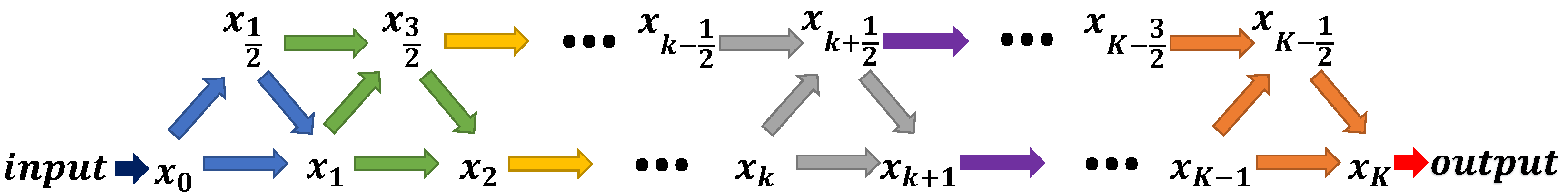
To summarize, our proposed extra proximal gradient network (EPGN) of a prescribed K phases is constructed by unrolling Algorithm 1, where each phase executes (6) but with (6c) and (6f) substituted by (11). The flowchart of the computation in EPGN is shown in Figure 1. The proposed EPGN not only inherits the advantages of Algorithm 1 but also employs learnable feature selection operations. Hence, EPGN combines the following properties: (i) the simple linear momentum layers (6a) and (6d) for improved convergence; (ii) the extra proximal gradient updates (6b), (6e), and (11) mimic the predictor–corrector scheme for parameter-efficient network structure; (iii) learnable feature extraction, selection, and residual resembling operators in (11) to effectively improve solution quality as the input data flows through EPGN.

Figure 1.
Overview of the K-phase extra proximal gradient network (EPGN) architecture. The arrows in the same color indicate computations within the same phase and share the same operators and parameters.
3.3. EPGN with Nonlocal Operator (NL-EPGN)
Nonlocal methods have proven effective for image reconstruction problems, such as in variational methods [35] and nonvariational approaches such as the notable BM3D algorithm [36]. Nonlocal operators can significantly improve image quality as they use image patches located in different regions to exploit the inherent self-similarity of images. Recently, the success of the nonlocal methods has motivated the investigation of the architecture of DNNs that have the ability to capture long-distance dependencies of the image. The deep network architecture for gray-scale and color image denoising in [37] is inspired by the projected gradient algorithm for solving a common variational image restoration model with a learnable nonlocal regularization. The nonlocal neural network proposed in [38] can be viewed as a generalization of the classical nonlocal mean in [35] that computes the response at a position as a weighted average of the image intensities at all positions. The weights implicitly depend on the feature maps in the patches with the size determined by the receptive fields.
To exploit repeated features in images for enhanced reconstruction quality, we adopt the idea in [38]. However, unlike [38] which only relies on nonlocal features, our NL-EPGN fuses local and nonlocal features of images using a combination operator learned through training data. More specifically, we propose NL-EPGN to integrate a nonlocal operator into the residual operator in (11), so that the features refined by the shrinkage operation can be passed to to leverage nonlocal features in images:
The operator contains two main components: a nonlocal block that extracts nonlocal features of the input, and a nonlinear layer that combines the local and nonlocal features. The details of these two components are given as follows.
3.3.1. Nonlocal Feature Extraction Block
Our design of the nonlocal feature extraction block follows the work [38] which computes a weighted average of features at all locations in an image. More precisely, let denote the input feature vector at position j and the response vector at position i of an image, then the nonlocal block computes by:
where the function computes a representation of the input signal at position j, and is the normalized weight depending on the similarity between and . The mapping corresponds to a learnable matrix (implemented as convolution). The weights are computed by embedded Gaussian:
where both and are implemented as convolutional filters of kernel size . We employ the bottleneck structure to reduce computation [38]. Hence, the nonlocal block in phase k is implemented as where
3.3.2. Local and Nonlocal Combination Layer
We propose to use a learnable combination layer of form to merge the input local feature and nonlocal feature obtained by nonlocal block in (15). That is, the nonlocal operator is defined by
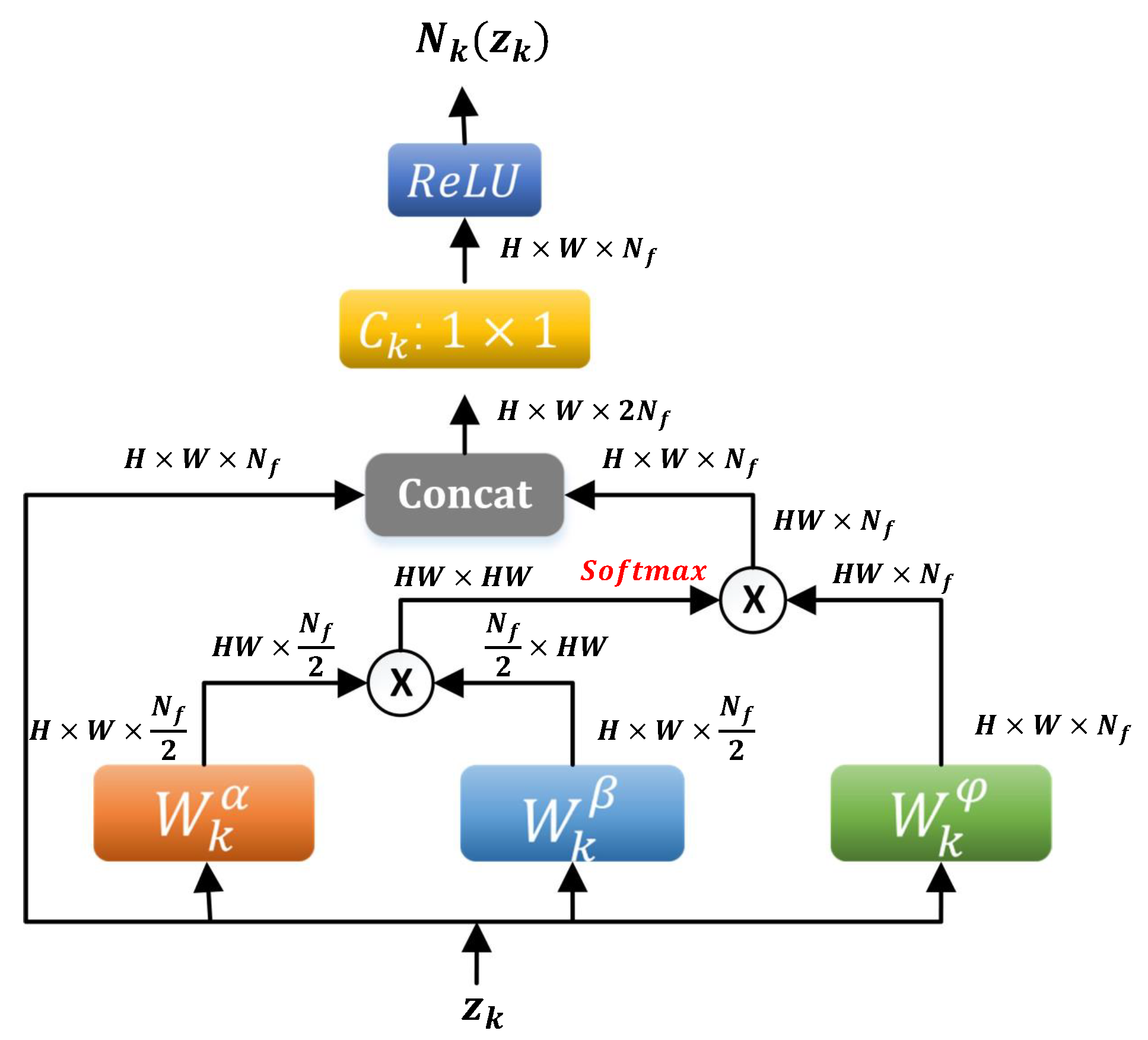
In the kth phase, the inputs of are for as shown in (12), stands for the concatenation operator at each pixel, and corresponds to a set of learnable weight vectors which project the concatenated vector to a scalar at each pixel (implemented as convolution). The flowchart of the nonlocal operator is shown in Figure 2.
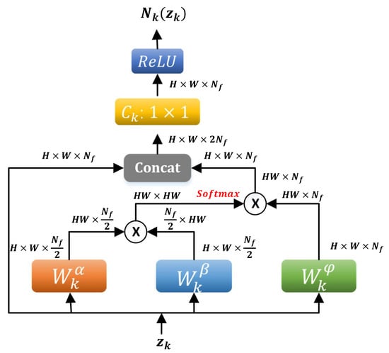
Figure 2.
Data flow in the nonlocal operator (16). “⨂” denotes matrix multiplication. Both input and output are of the same shape (height × width × #channel) of the image.
3.4. Network Training
As discussed above, the proposed EPGN (or NL-EPGN) consists of K phases, where each phase imitates one iteration in the accelerated extra gradient Algorithm 1 with proximal steps (6b) and (6e) replaced by (11) (or (12) for NL-EPGN). The flowchart of variables in the kth phase is shown in Figure 3. The parameters in the kth phase are collectively denoted by , which includes the feature extraction operator , the residual resembling operator , the nonlocal operator , the momentum coefficient , and the shrinkage thresholds . Let be the set of all network parameters. Then, given N training data pairs of form , where is the input measurement data and is the corresponding ground truth of the ith pair, we define the loss function of as
where denotes the output of the EPGN (i.e., the output of the last, Kth phase) parametrized by given input data . The optimal network parameter is obtained by minimizing the loss function (17) in the training process. After training, the EPGN with parameter serves as a feed-forward neural network that can reconstruct high-quality image given new measurement data on the fly.
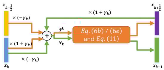
Figure 3.
Data flow in the kth phase of EPGN. “⨁” represents element-wise sum. Orange and green arrows represent computations in the first ((6a), (6b) and (11) with ) and second ((6d), (6e) and (11) with ) stages of EPGN, respectively.
4. Numerical Experiments
In this section, we evaluate the performance of the proposed EPGN and NL-EPGN on several inverse problems in imaging reconstruction applications. We focus on the reconstruction problem in compressive sensing in our experiments, however, the proposed method can be easily adapted to other image reconstruction problems by changing the data-fidelity term accordingly. All the experiments are implemented, trained, and tested in the TensorFlow framework [39] on a desktop with an Nvidia GTX-1080Ti GPU and 11 GB of graphics card memory (NVIDIA Corporation, Santa Clara, CA, USA).In all tests, the network parameters of EPGN/NL-EPGN are initialized using the Xavier method [40] and trained with the Adam optimizer [41] with learning rate for 200 epochs. To evaluate the reconstruction quality, we use the average peak signal-to-noise ratio (PSNR).
4.1. Nature Images Compressive Sensing
We first test EPGN on the compressive sensing (CS) image reconstruction problem. In our experiment we use the 91 Images dataset for training and Set11 for testing [42]. For a fair comparison, we follow the same data preparation and result evaluation procedures in [27]. The ground truth data contains image patches with luminance components that are all randomly cropped into size from 91 Images dataset. We then generate a matrix with random Gaussian entries of size and , where , and orthogonalize the rows. Then the measurement data for training is . The testing data Set11 preparation follows the same procedure as training data.
4.1.1. Comparison with Existing Methods
We set the phase number for EPGN and for NL-EPGN in this test (as shown in Figure 4 where the PSNRs of the networks become saturated). Table 1 shows the comparison of the average PSNRs of the images reconstructed by EPGN/NL-EPGN versus several state-of-the-art image reconstruction methods, namely TVAL3 [43], D-AMP [44], IRCNN [23], ReconNet [42], DR2-Net [45], ISTA-Net+ [27], and DPA-Net [46], where the first two are classical optimization-based methods, and the last five are deep learning-based methods. The PSNR results of the first four methods and ISTA-Net+ in Table 1 are quoted from [27]. We observe that EPGN and NL-EPGN outperform all aforementioned algorithms, whereas NL-EPGN obtains the highest accuracy.
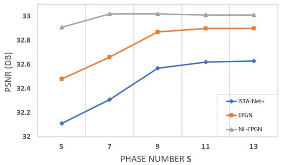
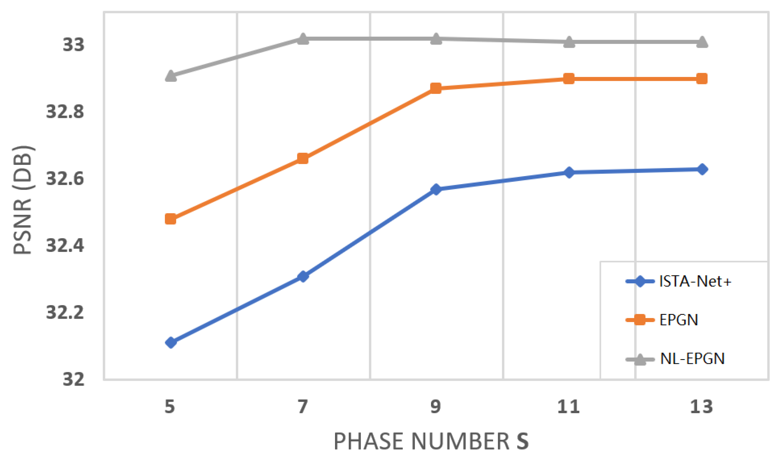
Figure 4.
Average PSNR comparison between ISTA-Net, EPGN and NL-EPGN with various phase number on image compressive sensing problem on Set11 with a CS ratio of .

Table 1.
Natural image CS reconstruction results by existing methods and the proposed EPGN (with 9 phases) and NL-EPGE (with 7 phases) on dataset Set11 with CS ratios of 10% and 25%. Table shows the average PSNR (dB) of the comparison methods.
4.1.2. Reconstruction Quality Assessment
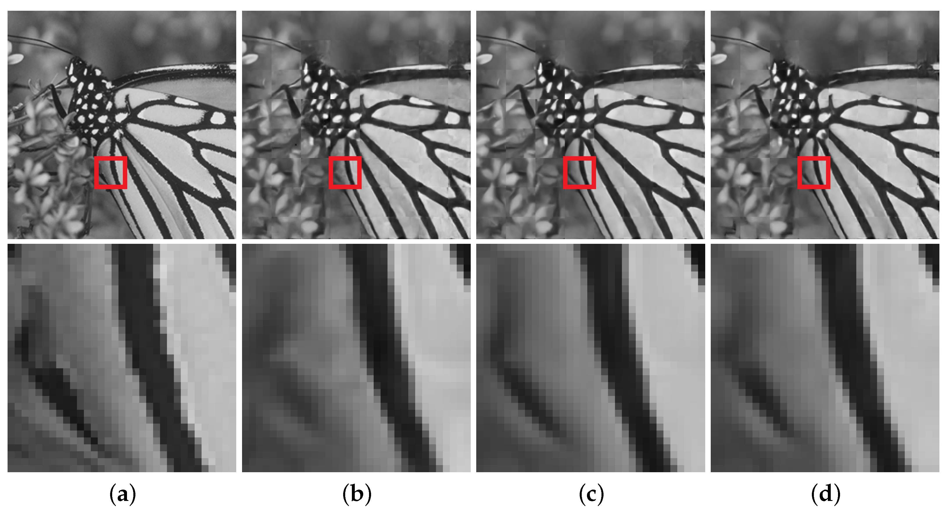
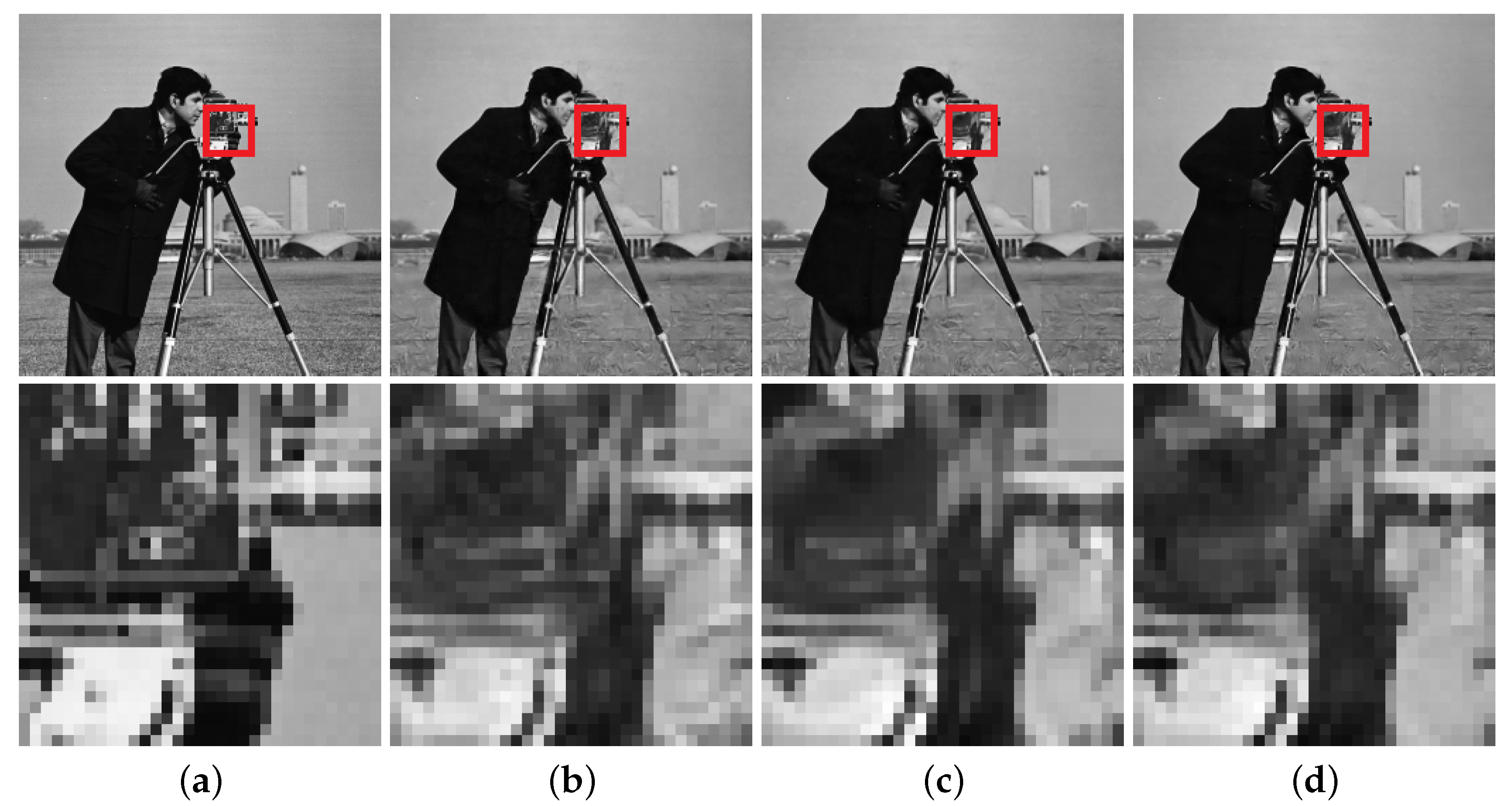
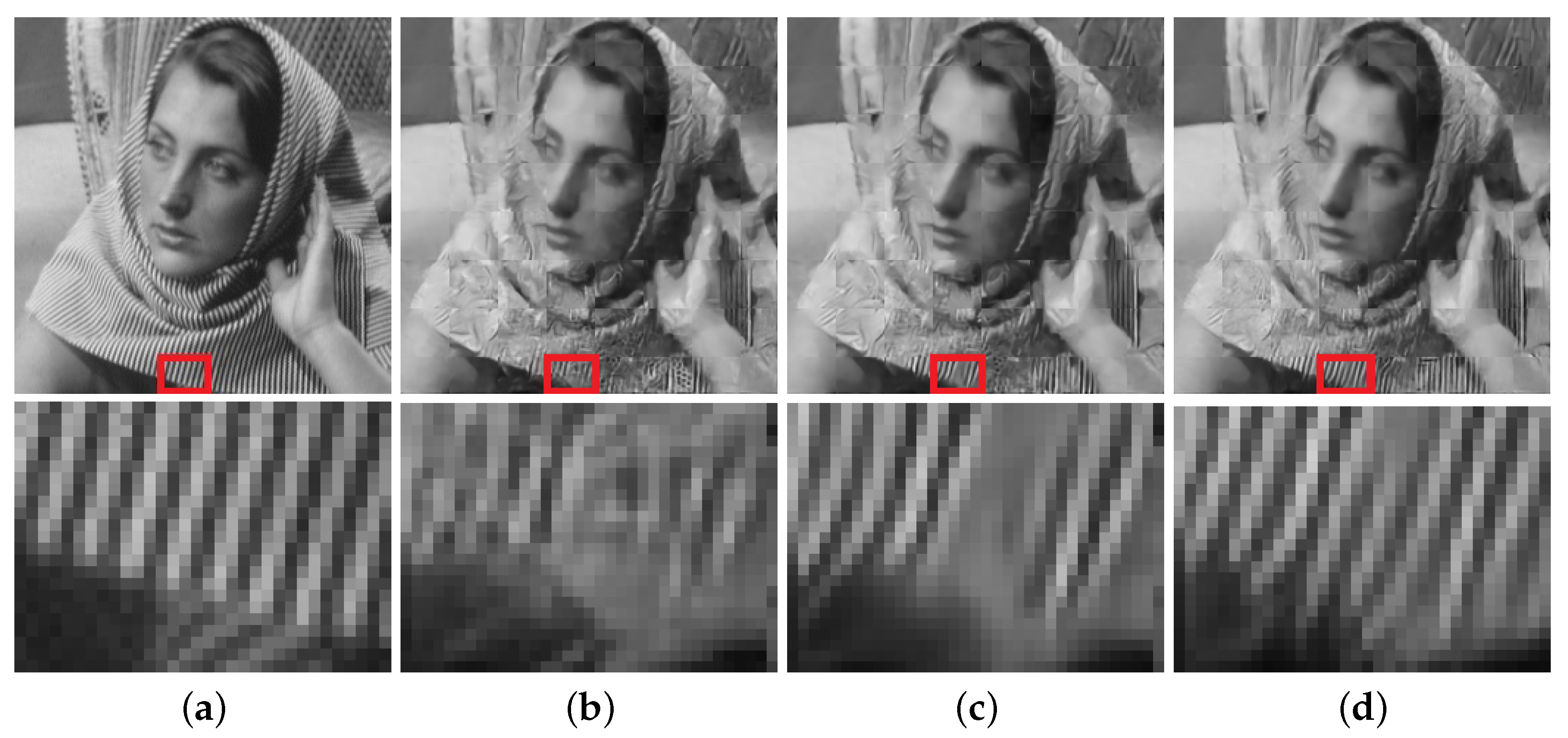
Compared to the state-of-the-art ISTA-Net+ [27], both EPGN and NL-EPGN obtain better reconstruction results with a similar number of parameters as shown in Table 2. In particular, Figure 5 shows the reconstructed butterfly image with a CS ratio of 10%, from which we can see that the 9-phase EPGN and 7-phase NL-EPGN can both capture the inconspicuous detail of the butterfly wings at the lower left part in the zoomed-in images. Similarly, Figure 6 shows the reconstructed cameraman image with a CS ratio of 25%, where the 9-phase EPGN and 7-phase NL-EPGN have fewer artifacts in the background compared to ISTA-Net+, as observed in the lower right area of the zoomed-in images. Figure 7 presents the reconstruction results of the Barbara image in Set11 from ISTA-Net+,the 9-phase EPGN, and the 7-phase NL-EPGN with a CS ratio of 10%. We can observe that the texture pattern of the scarf is better preserved by NL-EPGN due to the nonlocal operator.
Table 2.
Compressive sensing reconstruction performance comparison of the 9-phase ISTA-Net, 15-phase ISTA-Net, 9-phase EPGN, and 7-phase NL-EPGN on Set11 with a CS ratio of on the number of network parameters (# PARM), average PSNR in dB with standard deviation over the reconstructed images, and average reconstruction time (Time) of one image in second.
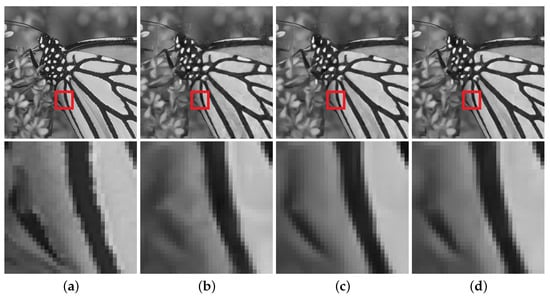
Figure 5.
Reconstruction of a butterfly image with a CS ratio of 10% using the 9-phase ISTA-Net (PSNR 25.91dB), 9-phase EPGN (26.47dB), and 7-phase NL-EPGN (26.58dB). (a) Ture. (b) ISTA-Net. (c) EPGN. (d) NL-EPGN.
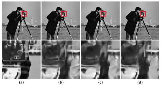
Figure 6.
Reconstruction of the cameraman image with a CS ratio 25% using the 9-phase ISTA-Net (PSNR 28.97dB), 9-phase EPGN (29.62dB), and 7-phase NL-EPGN (29.73dB). (a) Ture. (b) ISTA-Net. (c) EPGN. (d) NL-EPGN.
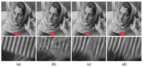
Figure 7.
Reconstruction of the Barbara image with a CS ratio of 10% using the 9-phase ISTA-Net (PSNR 23.59dB), 9-phase EPGN (23.89dB), and 7-phase NL-EPGN (24.27dB). (a) Ture. (b) ISTA-Net. (c) EPGN. (d) NL-EPGN.
4.1.3. Parameter Efficiency
The number of network parameters in each phase of ISTA-Net is [27]. The number of trainable parameters of each phase in EPGN is . Similarly, the number of learnable parameters of each phase in EPGN is . Therefore, the number of network parameters in each phase of ISTA-Net, EPGN, and NL-EPGN are very similar (NL-EPGN is about more than ISTA-Net and EPGN). Figure 4 shows the reconstruction PSNR of these three methods versus phase number, from which we observe that NL-EPGN becomes saturated with phase number , whereas EPGN with and ISTA-Net+ with . Nevertheless, as shown in Table 2, a 7-phase NL-EPGN has fewer network parameters than a 9-phase EPGN but achieves even higher PSNR.
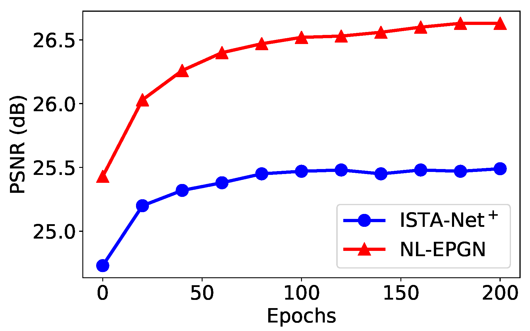
We compare the reconstruction results of EPGN and ISTA-Net in a range of different phase numbers with a CS ratio of , as shown in Figure 4. We observe that the PSNR values improve as the phase number increases and become saturated after . EPGN achieves a 0.3 dB higher PSNR on average than ISTA-Net. To further demonstrate the superiority of the extra proximal-gradient method over extending network depth, we compare the 9-phase EPGN with the 15-phase ISTA-Net, as shown in Table 2. Compared to the 15-phase ISTA-Net which extends the depth of the network by simply adding more phases, the 9-phase EPGN achieves better accuracy (0.27 dB higher) using much fewer parameters and similar reconstruction time. We compare the reconstruction performance of EPGN and NL-EPGN with CS ratios of 10% and 25%, the 7-phase NL-EPGN outperforms the 9-phase EPGN by 0.21 dB and 0.15 dB respectively, as shown in Table 1. We also compare the reconstruction results of NL-EPGN and EPGN in a range of different phase numbers with a CS ratio of 25%. The results are shown in Figure 4. We observe that NL-EPGN achieves an average of 0.2 dB PSNR better than EPGN. It is interesting that the PSNR of NL-EPGN shows no significant improvement after . As shown in Table 2, the reconstruction time of the 7-phase NL-EPGN is approximate 7 to 8 times that of the 9-phase EPGN due to the time complexity of the nonlocal operator. However, the effect of the nonlocal operator is remarkable, NL-EPGN with 7 phases has a 0.15 dB PSNR improvement with 13.7% fewer parameters compared to EPGN with 9 phases. In Figure 8, we show the PSNR versus epoch using the proposed NL-EPGN and the state-of-the-art method ISTA-Net for image reconstruction with a CS ratio of 10% and phase number 3. While both networks gradually improve PSNR with more epochs, NL-EPGN appears to be significantly more effective than ISTA-Net during training as the former produces reconstructions with much higher PSNR.
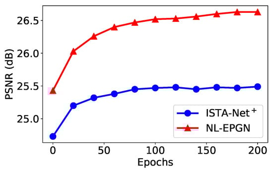
Figure 8.
Average PSNR comparison between ISTA-Net and NL-EPGN with various numbers of epochs during training with 3 phases on Set11 with a CS ratio of .
4.2. MR Images Compressive Sensing
We also test the performance of EPGN on compressive sensing reconstruction of brain MR images [47] (CS-MRI). We randomly selected 100 and 50 images for training and testing, respectively, and cropped every image to the size of . In the CS-MRI problem, the data fidelity is , where , P is a binary selection matrix representating the sampling trajectory, and is the discrete Fourier transform. We compare EPGN with ISTA-Net [27] on the same MRI data set. The experimental results on various undersampling ratios of radial masks are summarized in Table 3. Here, we set the phase number of ISTA-Net and EPGN to 15 and 11 respectively. It is obvious that EPGN outperforms ISTA-Net for each undersampling ratio.
Table 3.
PSNR (dB) of reconstructions obtained by ISTA-Net and EPGN on MR images using radial masks with sampling ratios of 10%, 20%, and 30%.
5. Concluding Remarks
We presented a novel deep neural network architecture, called the extra proximal gradient network (EPGN), to solve a general class of inverse problems with a focus on image reconstruction applications. EPGN imitates the accelerated extra proximal gradient algorithm and features a learned regularization that incorporates adaptive sparsification mappings, robust shrinkage selections, and the combination of local and nonlocal operators for improved solution quality and network parameter efficiency. Extensive numerical experiments show that EPGN outperforms several existing state-of-the-art methods on a variety of image reconstruction problems.
Author Contributions
Conceptualization, X.Y. and Y.C.; Data curation, Q.Z.; Formal analysis, X.Y. and Y.C.; Funding acquisition, Y.C.; Investigation, Q.Z., X.Y. and Y.C.; Methodology, Q.Z., X.Y. and Y.C.; Project administration, Y.C.; Resources, Y.C.; Software, Q.Z.; Supervision, Y.C.; Validation, Q.Z.; Visualization, Q.Z.; Writing—original draft, Q.Z., X.Y. and Y.C.; Writing—review & editing, X.Y. and Y.C. All authors have read and agreed to the published version of the manuscript.
Funding
This work was supported in part by National Science Foundation under grants DMS-1818886, DMS-1925263, DMS-2152960, and DMS-2152961.
Informed Consent Statement
Informed consent was obtained from all subjects involved in the study.
Data Availability Statement
The MRI data presented in this study are available on 2013 Diencephalon Free Challenge [47] at https://my.vanderbilt.edu/masi/workshops/ (accessed on 5 April 2022) and the nature image data are available at https://people.ee.ethz.ch/~timofter/ (accessed on 5 April 2022).
Conflicts of Interest
The authors declare no conflict of interest.
References
- Krizhevsky, A.; Sutskever, I.; Hinton, G.E. ImageNet Classification with Deep Convolutional Neural Networks. In Proceedings of the 26th Annual Conference on Neural Information Processing Systems 2012, Lake Tahoe, NV, USA, 3–6 December 2012. Advances in Neural Information Processing Systems 25. [Google Scholar]
- Girshick, R.; Donahue, J.; Darrell, T.; Malik, J. Rich feature hierarchies for accurate object detection and semantic segmentation. In Proceedings of the IEEE Conference on Computer Vision and Pattern Recognition, Columbus, OH, USA, 23–28 June 2014; pp. 580–587. [Google Scholar]
- Yang, W.; Zhang, X.; Tian, Y.; Wang, W.; Xue, J.H.; Liao, Q. Deep learning for single image super-resolution: A brief review. IEEE Trans. Multimed. 2019, 21, 3106–3121. [Google Scholar] [CrossRef] [Green Version]
- Chen, Y.; Ye, X.; Zhang, Q. Variational Model-Based Deep Neural Networks for Image Reconstruction. In Handbook of Mathematical Models and Algorithms in Computer Vision and Imaging: Mathematical Imaging and Vision; Chen, K., Schönlieb, C.B., Tai, X.C., Younces, L., Eds.; Springer International Publishing: Cham, Switzerland, 2021; pp. 1–29. [Google Scholar] [CrossRef]
- Wan, M.; Zha, D.; Liu, N.; Zou, N. Modeling Techniques for Machine Learning Fairness: A Survey. arXiv 2021, arXiv:2111.03015. [Google Scholar]
- Young, T.; Hazarika, D.; Poria, S.; Cambria, E. Recent trends in deep learning based natural language processing. IEEE Comput. Intell. Mag. 2018, 13, 55–75. [Google Scholar] [CrossRef]
- Tian, H.; Jiang, X.; Trozzi, F.; Xiao, S.; Larson, E.C.; Tao, P. Explore Protein Conformational Space With Variational Autoencoder. Front. Mol. Biosci. 2021, 8, 781635. [Google Scholar] [CrossRef]
- Litjens, G.; Kooi, T.; Bejnordi, B.E.; Setio, A.A.A.; Ciompi, F.; Ghafoorian, M.; Van Der Laak, J.A.; Van Ginneken, B.; Sánchez, C.I. A survey on deep learning in medical image analysis. Med. Image Anal. 2017, 42, 60–88. [Google Scholar] [CrossRef] [Green Version]
- Hesamian, M.H.; Jia, W.; He, X.; Kennedy, P. Deep learning techniques for medical image segmentation: Achievements and challenges. J. Digit. Imaging 2019, 32, 582–596. [Google Scholar] [CrossRef] [Green Version]
- Lu, Z.; Pu, H.; Wang, F. The expressive power of neural networks: A view from the width. In Proceedings of the Thirty-First Conference on Neural Information Processing Systems, Long Beach, CA, USA, 4–9 December 2017; pp. 6231–6239. [Google Scholar]
- Tibshirani, R. Regression Shrinkage and Selection via the Lasso. J. R. Stat. Soc. Ser. B Methodol. 1996, 58, 267–288. [Google Scholar] [CrossRef]
- Zhang, B.; Fu, Y.; Lu, Y.; Zhang, Z.; Clarke, R.; Van Eyk, J.E.; Herrington, D.M.; Wang, Y. DDN2.0: R and Python packages for differential dependency network analysis of biological systems. bioRxiv 2021. [Google Scholar] [CrossRef]
- Bao, R.; Gu, B.; Huang, H. Efficient Approximate Solution Path Algorithm for Order Weight L1-Norm with Accuracy Guarantee. In Proceedings of the 2019 IEEE International Conference on Data Mining (ICDM), Beijing, China, 8–11 November 2019; pp. 958–963. [Google Scholar] [CrossRef]
- Gregor, K.; LeCun, Y. Learning Fast Approximations of Sparse Coding. In Proceedings of the 27th International Conference on Machine Learning (ICML 2010), Haifa, Israel, 21–24 June 2010; pp. 399–406. [Google Scholar]
- Chen, X.; Liu, J.; Wang, Z.; Yin, W. Theoretical linear convergence of unfolded ISTA and its practical weights and thresholds. In Proceedings of the Thirty-second Annual Conference on Neural Information Processing Systems (NIPS), Montreal, QC, Canada, 3–8 December 2018; pp. 9061–9071. [Google Scholar]
- Liu, J.; Chen, X.; Wang, Z.; Yin, W. ALISTA: Analytic weights are as good as learned weights in LISTA. In Proceedings of the International Conference on Learning Representations (ICLR), New Orleans, LA, USA, 6–9 May 2019. [Google Scholar]
- Sprechmann, P.; Bronstein, A.M.; Sapiro, G. Learning efficient sparse and low rank models. TPAMI 2015, 37, 1821–1833. [Google Scholar] [CrossRef]
- Xin, B.; Wang, Y.; Gao, W.; Wipf, D.; Wang, B. Maximal sparsity with deep networks? In Proceedings of the Thirtieth Conference on Neural Information Processing Systems (NIPS), Barcelona, Spain, 5–10 December 2016; pp. 4340–4348. [Google Scholar]
- Borgerding, M.; Schniter, P.; Rangan, S. AMP-inspired deep networks for sparse linear inverse problems. IEEE Trans. Signal Process. 2017, 65, 4293–4308. [Google Scholar] [CrossRef]
- Xie, X.; Wu, J.; Zhong, Z.; Liu, G.; Lin, Z. Differentiable Linearized ADMM. arXiv 2019, arXiv:1905.06179. [Google Scholar]
- Bao, R.; Gu, B.; Huang, H. Fast OSCAR and OWL Regression via Safe Screening Rules. In Proceedings of the 37th International Conference on Machine Learning, Virtual Event, 12–18 July 2020; pp. 653–663. [Google Scholar]
- He, K.; Zhang, X.; Ren, S.; Sun, J. Deep residual learning for image recognition. In Proceedings of the 2016 IEEE Conference on Computer Vision and Pattern Recognition (CVPR), Las Vegas, NV, USA, 26–30 June 2016; pp. 770–778. [Google Scholar]
- Zhang, K.; Zuo, W.; Gu, S.; Zhang, L. Learning deep CNN denoiser prior for image restoration. In Proceedings of the 2017 IEEE Conference on Computer Vision and Pattern Recognition (CVPR), Honolulu, HI, USA, 22–25 July 2017; pp. 3929–3938. [Google Scholar]
- Chang, J.R.; Li, C.L.; Poczos, B.; Kumar, B.V. One network to solve them all: Solving linear inverse problems using deep projection models. In Proceedings of the 2017 IEEE International Conference on Computer Vision (ICCV), Venice, Italy, 22–29 October 2017; pp. 5889–5898. [Google Scholar]
- Meinhardt, T.; Moller, M.; Hazirbas, C. Learning proximal operators: Using denoising networks for regularizing inverse imaging problems. In Proceedings of the 2017 IEEE International Conference on Computer Vision (ICCV), Venice, Italy, 22–29 October 2017; pp. 1781–1790. [Google Scholar]
- Yang, Y.; Sun, J.; Li, H.; Xu, Z. Deep ADMM-Net for Compressive Sensing MRI. In Proceedings of the Thirtieth Conference on Neural Information Processing Systems (NIPS), Barcelona, Spain, 5–10 December 2016; pp. 10–18. [Google Scholar]
- Zhang, J.; Ghanem, B. ISTA-Net: Interpretable Optimization-Inspired Deep Network for Image Compressive Sensing. In Proceedings of the 2018 IEEE Conference on Computer Vision and Pattern Recognition (CVPR), Salt Lake City, UT, USA, 18–22 June 2018. [Google Scholar]
- Korpelevi, G.M. An extragradient method for finding saddle points and for other problems. Ekon. Mate. Metody 1976, 12, 747–756. [Google Scholar]
- Censor, Y.; Gibali, A.; Reich, S. The subgradient extragradient method for solving variational inequalities in Hilbert space. J. Optim. Theory Appl. 2011, 148, 318–335. [Google Scholar] [CrossRef] [PubMed] [Green Version]
- Nguyen, T.P.; Pauwels, E.; Richard, E.; Suter, B.W. Extragradient method in optimization: Convergence and complexity. J. Optim. Theory Appl. 2018, 176, 137–162. [Google Scholar] [CrossRef] [Green Version]
- Diakonikolas, J.; Orecchia, L. Accelerated Extra-Gradient Descent: A Novel Accelerated First-Order Method. In Proceedings of the 9th Annual Innovations in Theoretical Computer Science (ITCS) Conference, Cambridge, MA, USA, 11–14 January 2018; pp. 23:1–23:19. [Google Scholar] [CrossRef]
- Nesterov, Y. Introductory Lectures on Convex Optimization: A Basic Course, 1st ed.; Springer: Berlin/Heidelberg, Germany, 2014. [Google Scholar]
- Li, H.; Lin, Z. Accelerated proximal gradient methods for nonconvex programming. In Proceedings of the Advances in Neural Information Processing Systems 28 (NIPS 2015), Montréal, QC, Canada, 7–12 December 2015; pp. 379–387. [Google Scholar]
- Le, H.; Borji, A. What are the Receptive, Effective Receptive, and Projective Fields of Neurons in Convolutional Neural Networks? arXiv 2017, arXiv:abs/1705.07049. [Google Scholar]
- Buades, A.; Coll, B.; Morel, J.M. A non-local algorithm for image denoising. In Proceedings of the 2005 IEEE Computer Society Conference on Computer Vision and Pattern Recognition (CVPR), San Diego, CA, USA, 20–26 June 2005; pp. 60–65. [Google Scholar]
- Dabov, K.; Foi, A.; Katkovnik, V.; Egiazarian, K. Image denoising by sparse 3-D transform-domain collaborative filtering. IEEE Trans. Image Process. 2007, 16, 2080–2095. [Google Scholar] [CrossRef]
- Lefkimmiatis, S. Non-local color image denoising with convolutional neural networks. In Proceedings of the 2017 IEEE Conference on Computer Vision and Pattern Recognition (CVPR), Honolulu, HI, USA, 22–25 July 2017; pp. 3587–3596. [Google Scholar]
- Wang, X.; Girshick, R.; Gupta, A.; He, K. Non-local neural networks. In Proceedings of the 2018 IEEE Conference on Computer Vision and Pattern Recognition (CVPR), Salt Lake City, UT, USA, 18–22 June 2018; pp. 7794–7803. [Google Scholar]
- Abadi, M.; Barham, P.; Chen, J. Tensorflow: A system for large-scale machine learning. In Proceedings of the 12th USENIX Symposium on Operating Systems Design and Implementation, Savannah, GA, USA, 2–4 November 2016; pp. 265–283. [Google Scholar]
- Glorot, X.; Bengio, Y. Understanding the difficulty of training deep feedforward neural networks. In Proceedings of the 13th International Conference on Artificial Intelligence and Statistics, Sardinia, Italy, 13–15 May 2010. [Google Scholar]
- Kingma, D.; Ba, J. Adam: A method for stochastic optimization. arXiv 2014, arXiv:1412.6980. [Google Scholar]
- Kulkarni, K.; Lohit, S.; Turaga, P. Reconnet: Non-iterative reconstruction of images from compressively sensed measurements. In Proceedings of the 2016 IEEE Conference on Computer Vision and Pattern Recognition (CVPR), Las Vegas, NV, USA, 26–30 June 2016; pp. 449–458. [Google Scholar]
- Li, C.; Yin, W.; Jiang, H. An efficient augmented Lagrangian method with applications to total variation minimization. Comput. Optim. Appl. 2013, 56, 507–530. [Google Scholar] [CrossRef] [Green Version]
- Metzler, C.; Maleki, A.; Baraniuk, R. From denoising to compressed sensing. IEEE Trans. Inf. Theory 2016, 62, 5117–5144. [Google Scholar] [CrossRef]
- Yao, H.; Dai, F.; Zhang, S.; Zhang, Y.; Tian, Q.; Xu, C. DR2-Net: Deep residual reconstruction network for image compressive sensing. Neurocomputing 2019, 359, 483–493. [Google Scholar] [CrossRef] [Green Version]
- Sun, Y.; Chen, J.; Liu, Q.; Liu, B.; Guo, G. Dual-Path Attention Network for Compressed Sensing Image Reconstruction. IEEE Trans. Image Process. 2020, 29, 9482–9495. [Google Scholar] [CrossRef] [PubMed]
- Landman, B.; Warfield, S. (Eds.) 2013 Diencephalon Free Challenge; Sage Bionetworks: Seattle, WA, USA, 2013. [Google Scholar] [CrossRef]

Publisher’s Note: MDPI stays neutral with regard to jurisdictional claims in published maps and institutional affiliations. |
© 2022 by the authors. Licensee MDPI, Basel, Switzerland. This article is an open access article distributed under the terms and conditions of the Creative Commons Attribution (CC BY) license (https://creativecommons.org/licenses/by/4.0/).