
Airborne Hyperspectral Imagery for Band Selection Using Moth–Flame Metaheuristic Optimization


Abstract
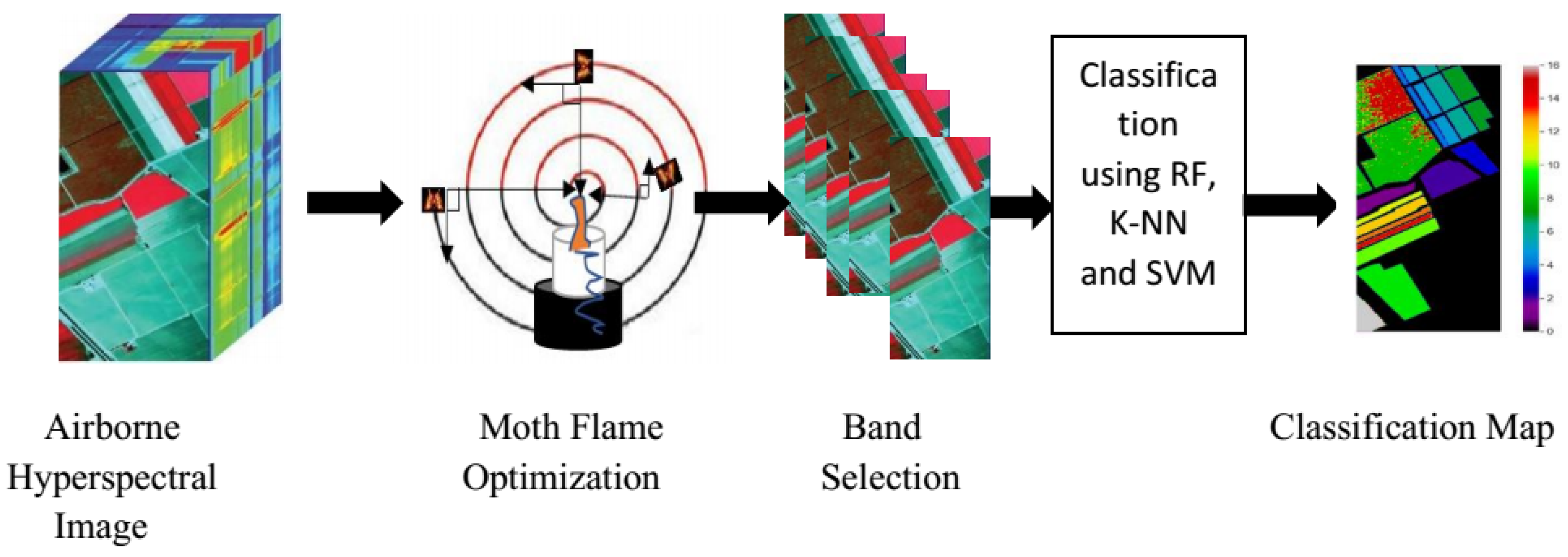
:1. Introduction
- We propose an MFO-based algorithm for hyperspectral band selection.
- We implemented and tested MFO-based hyperspectral band selection for three benchmark datasets.
- We compared the performance of MFO with three state-of-the-art metaheuristic band selection methods.
2. Materials and Methods
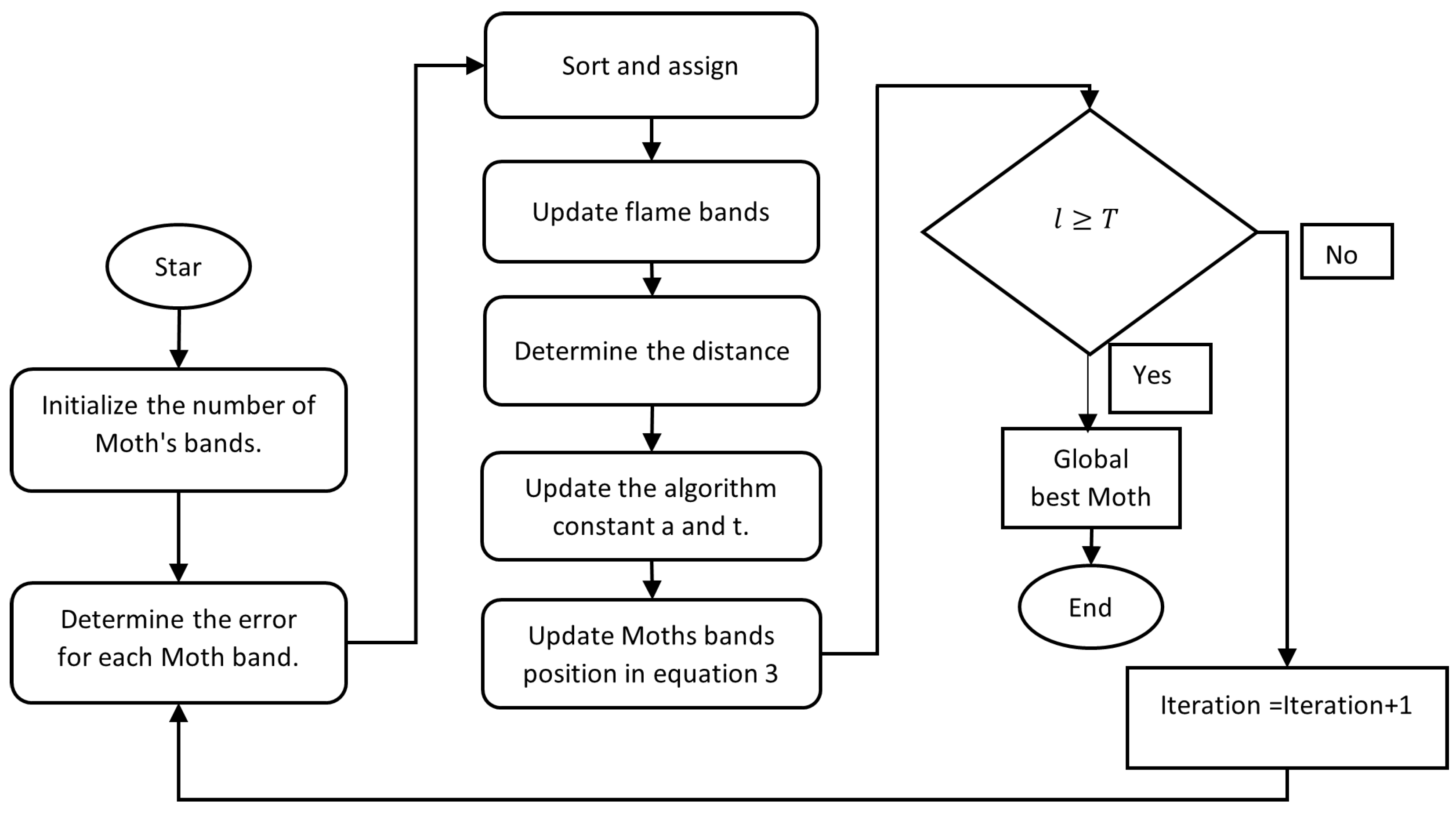
Moth–Flame Optimization Algorithm
| Algorithm 1: Optimal band selection from airborne HSI using moth–flame optimization. |
Input: Train and test datasets from Output: Band collection derived from the HSI data cube using MFO’s global optimum location. Procedure MFO Algorithm Moths are generated randomly at first to populate the feasible search space Evaluate and classify the fitness of the entire population Equal to the sorted population in flames While iteration < max iteration The following equation can be used to calculate the flame number.
The distance between the moth concerning its corresponding flame can be obtained from: Update the value of constant a and t.
Update and sort the fitness for all search agents. Update the flames. Iteration = Iteration + 1. End while To find the global best position |
3. Classification Methods
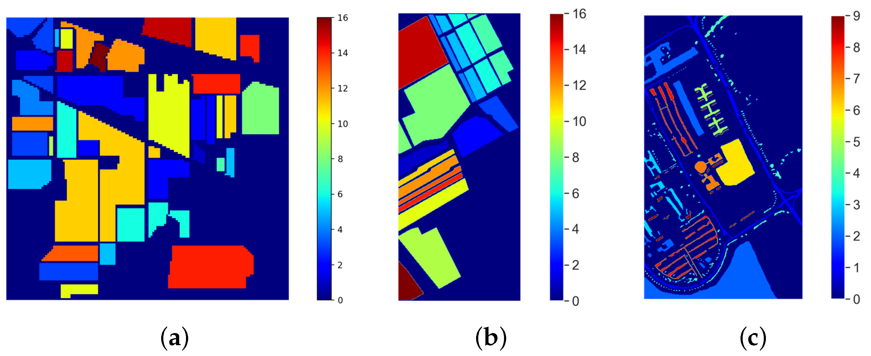
Dataset Description
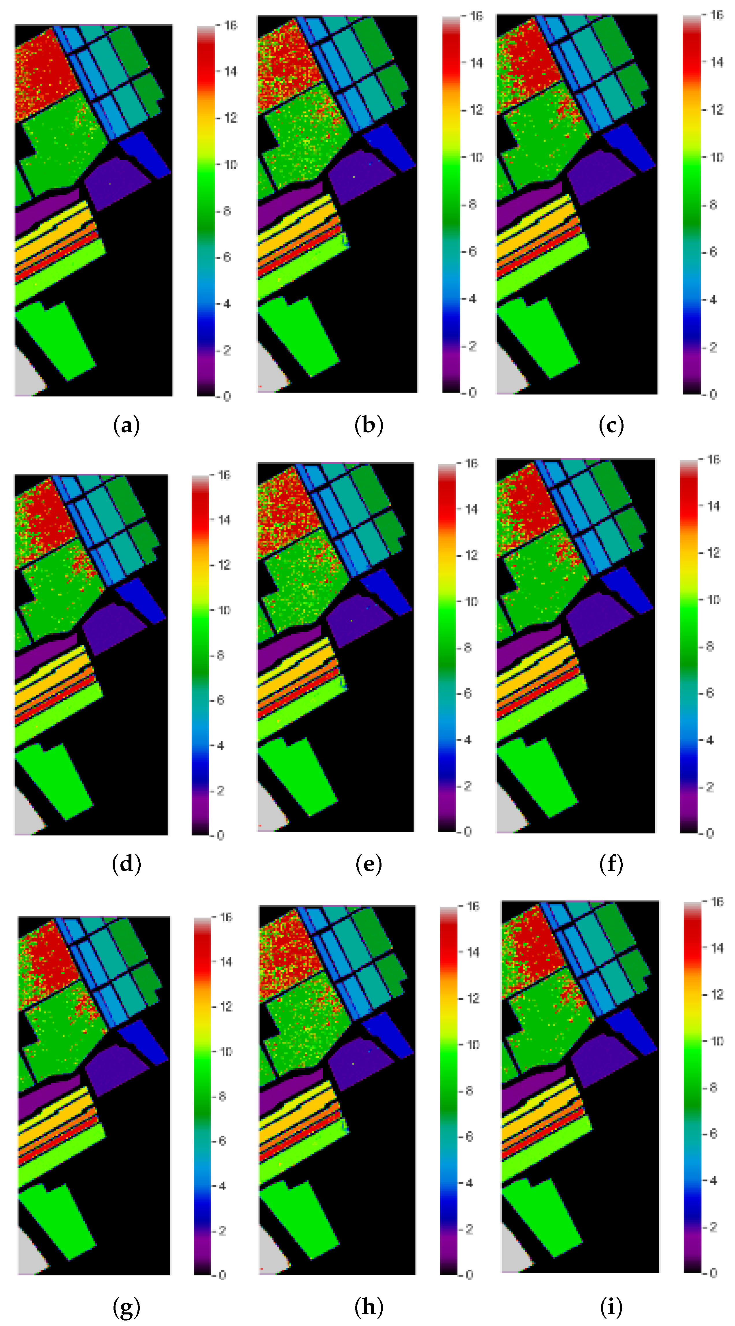
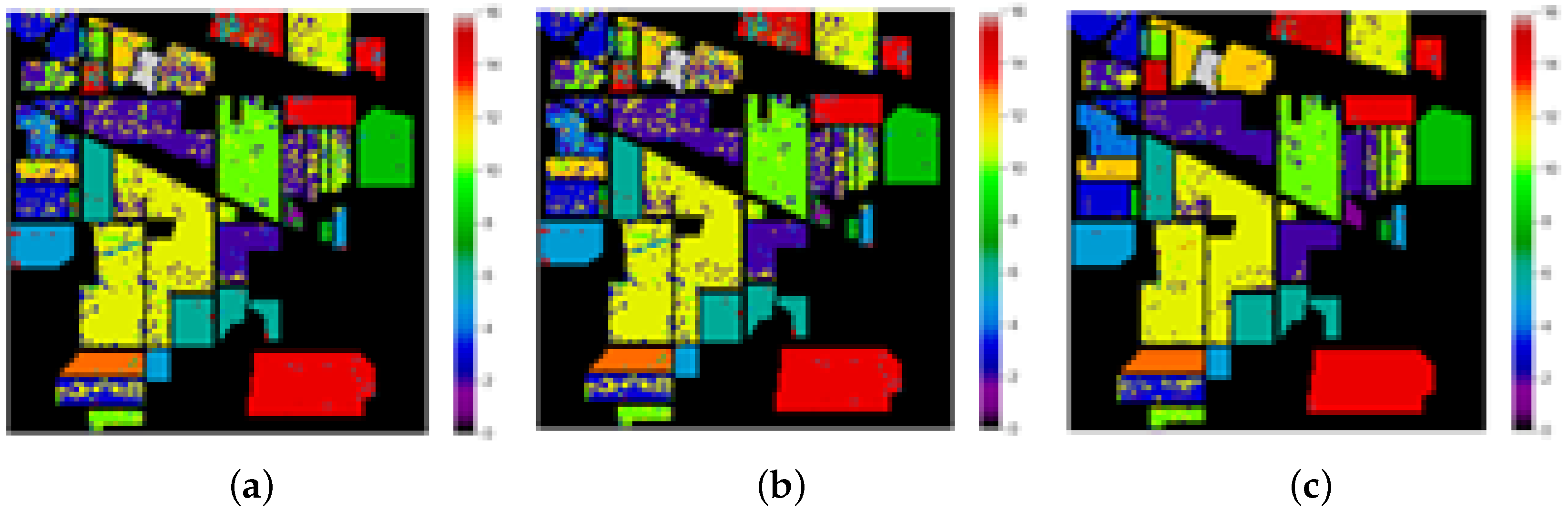
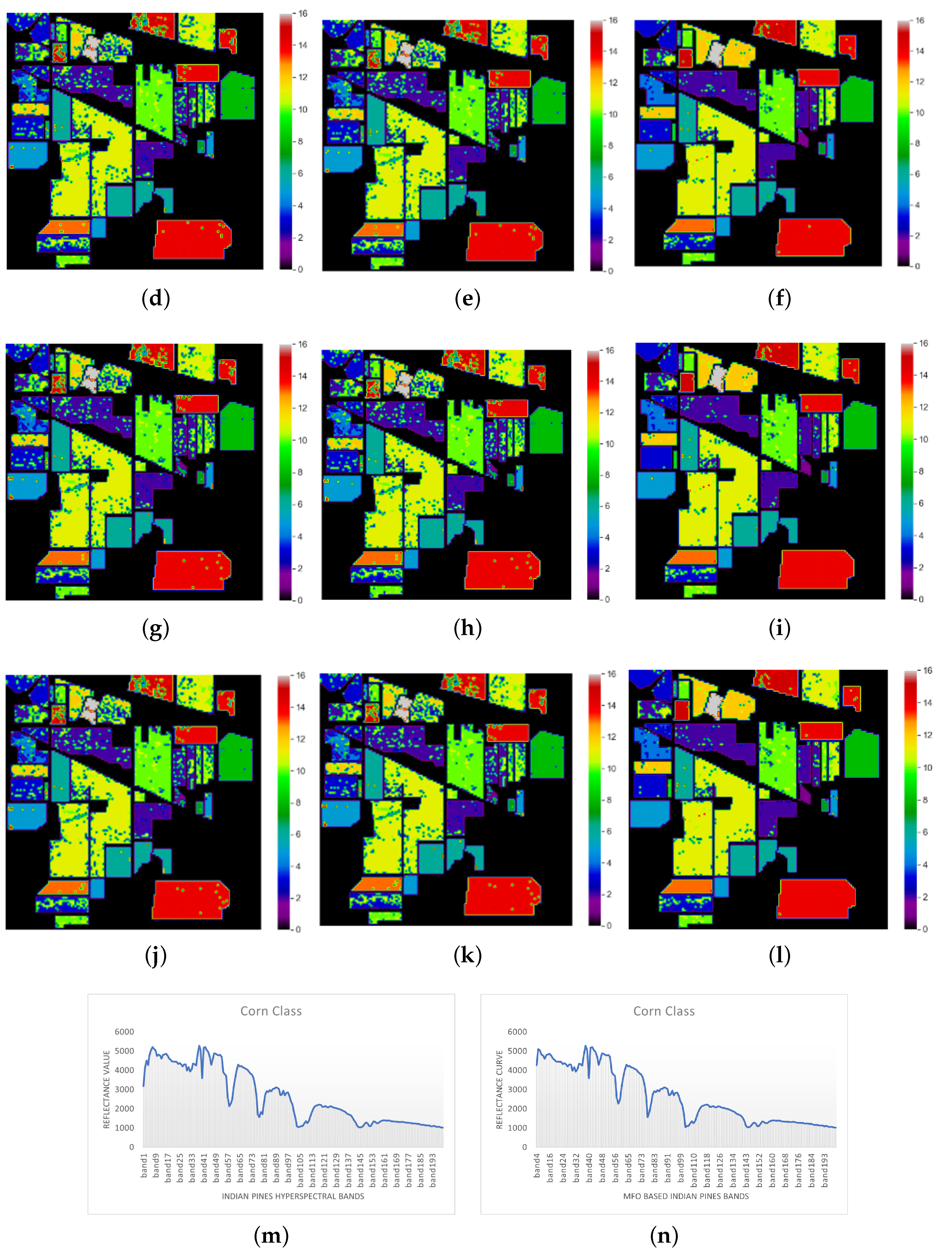
4. Experimental Results
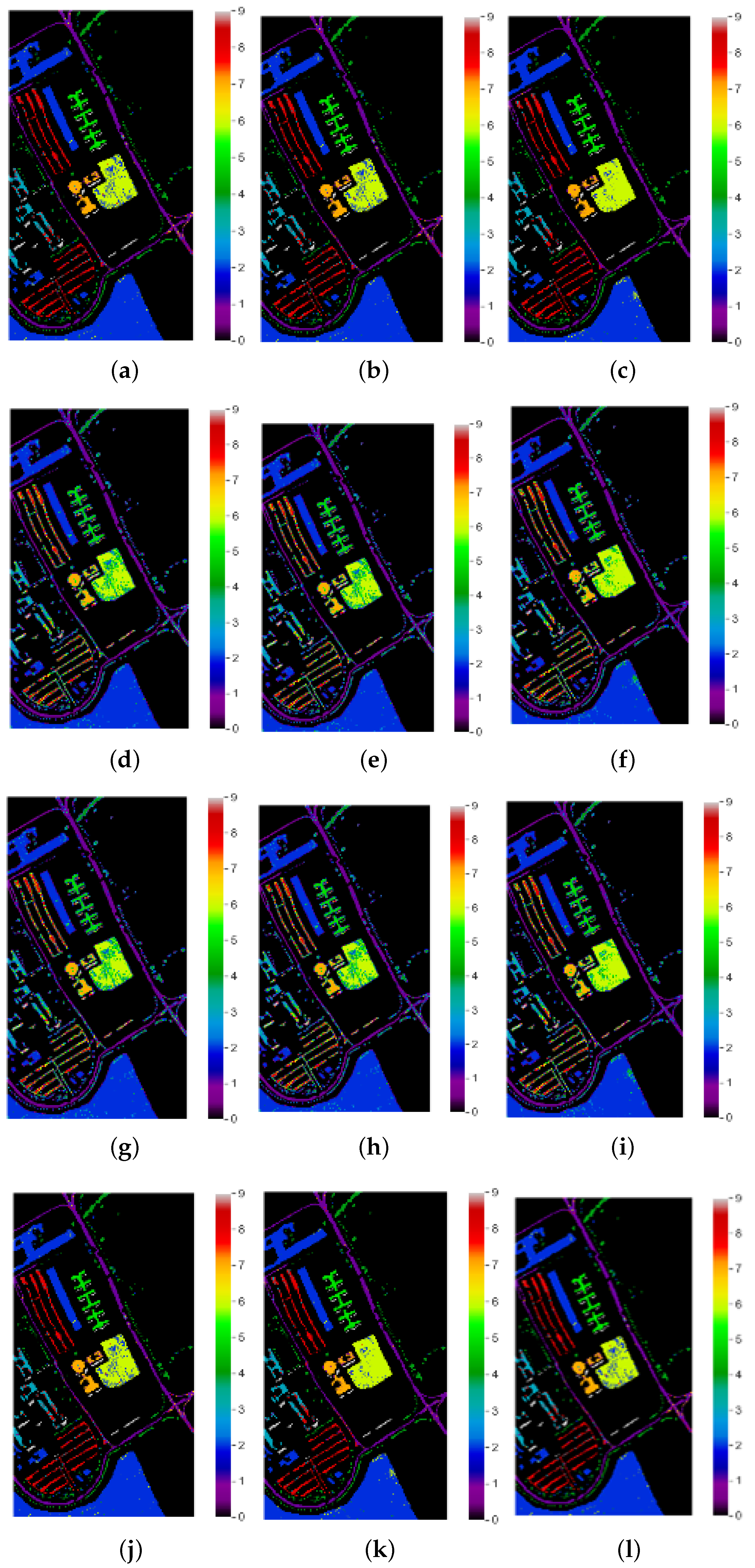
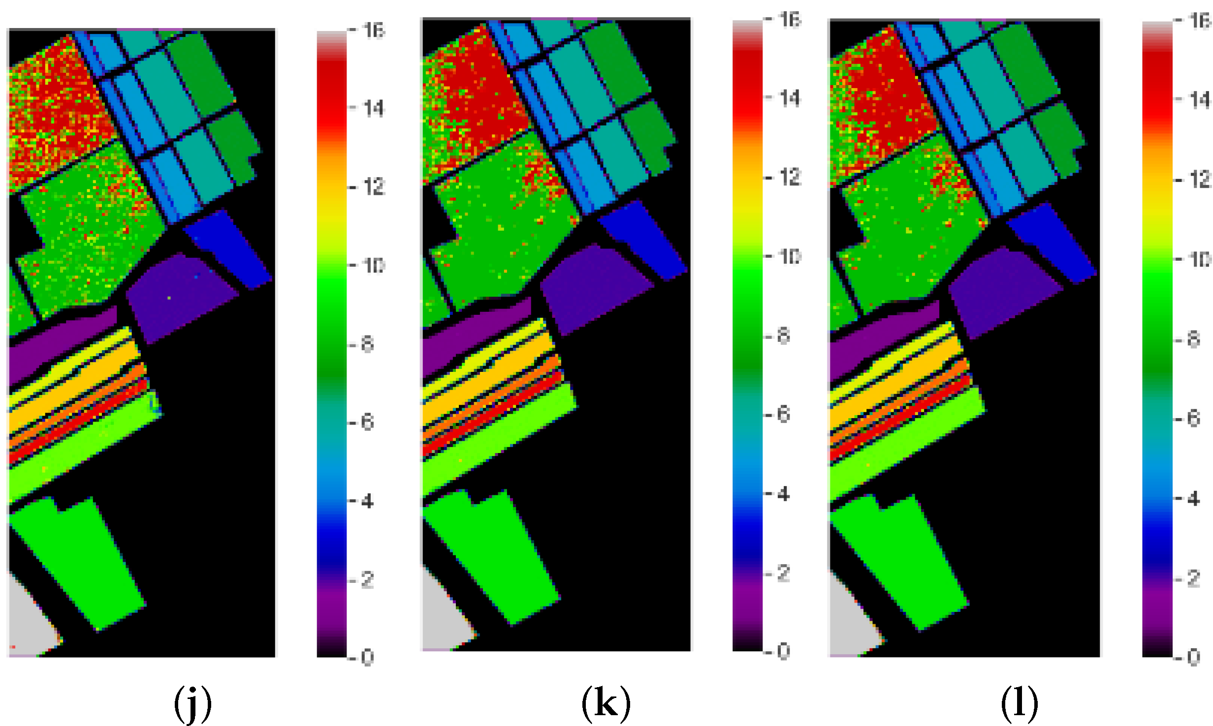
Classification Maps
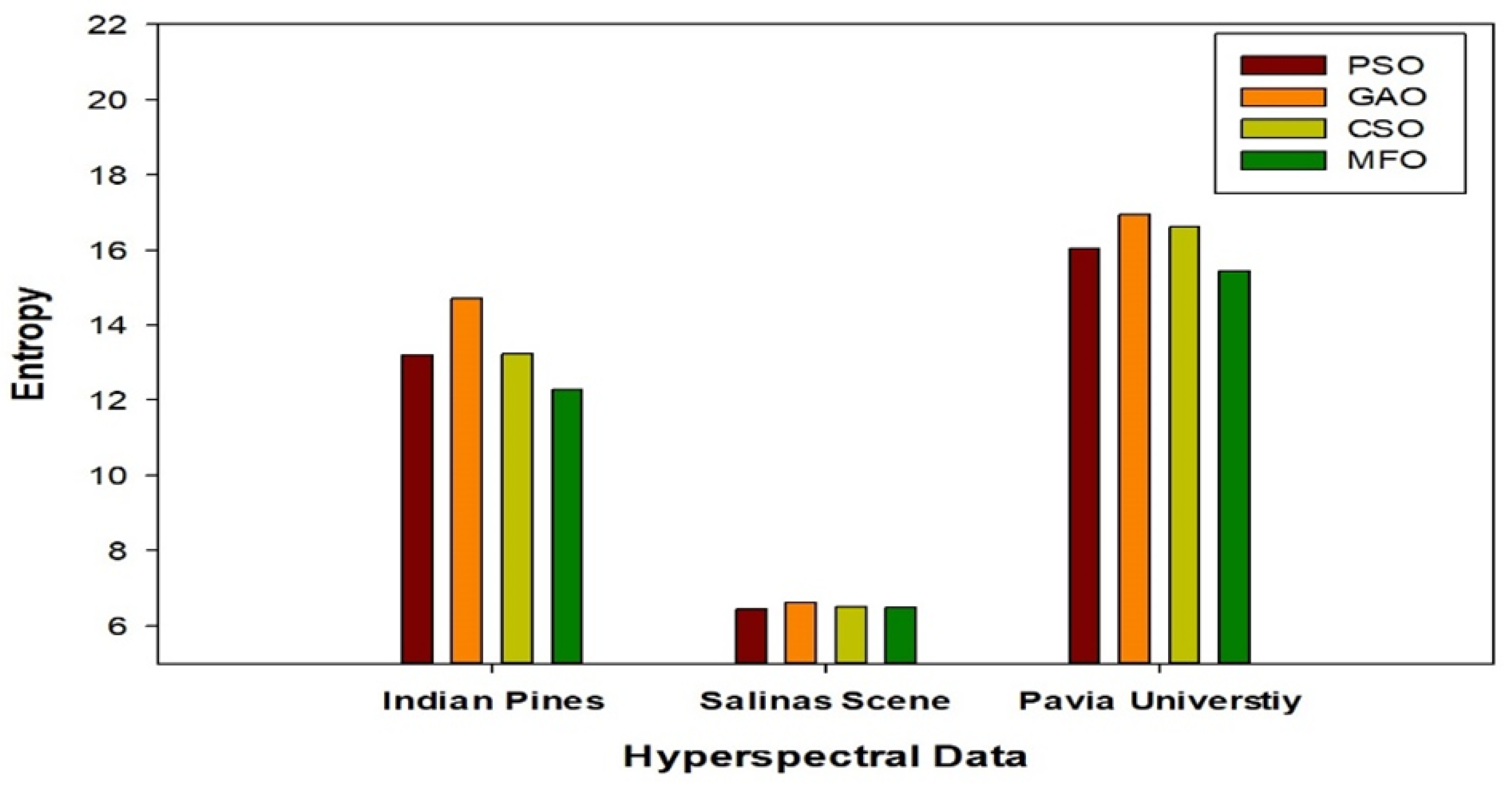
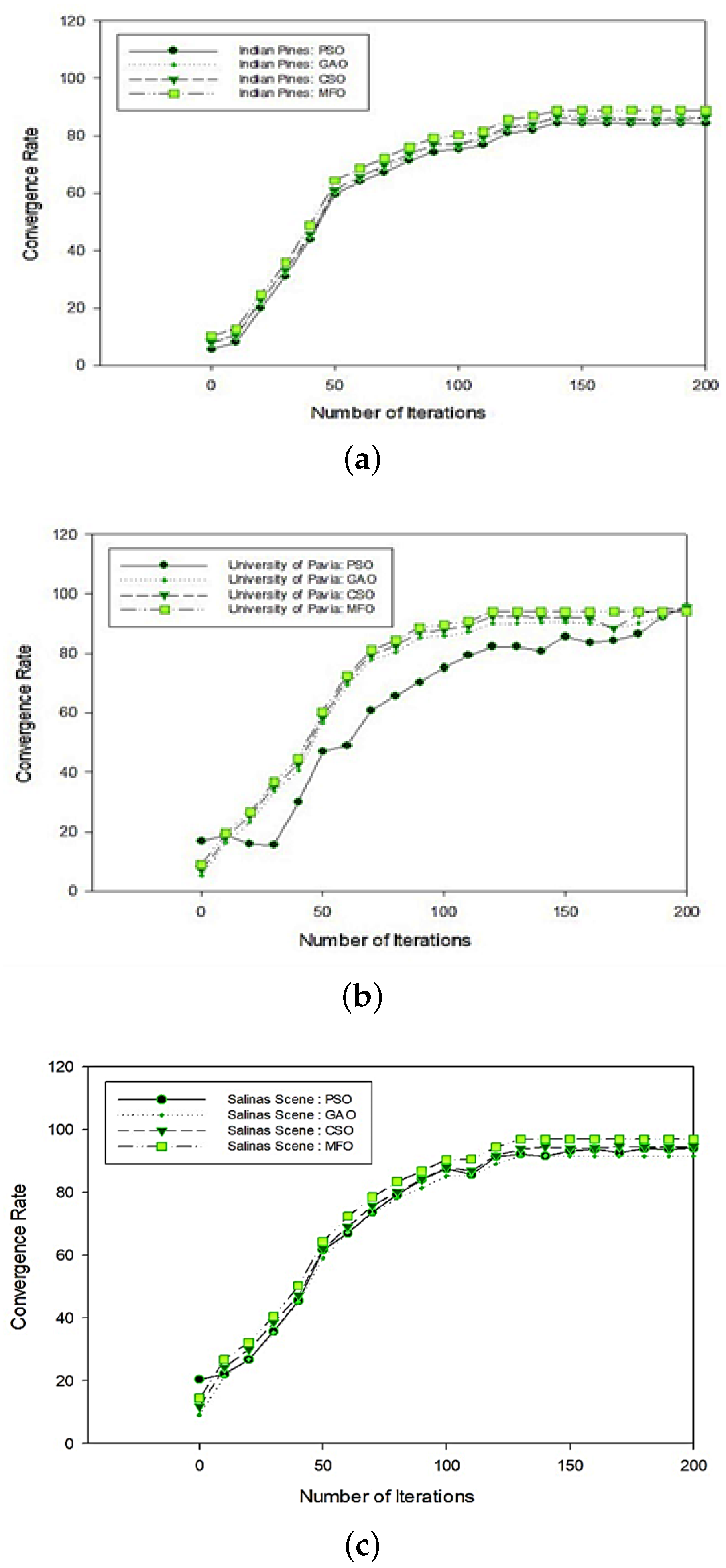
5. Comparative Analysis of State-of-the-Art Approaches
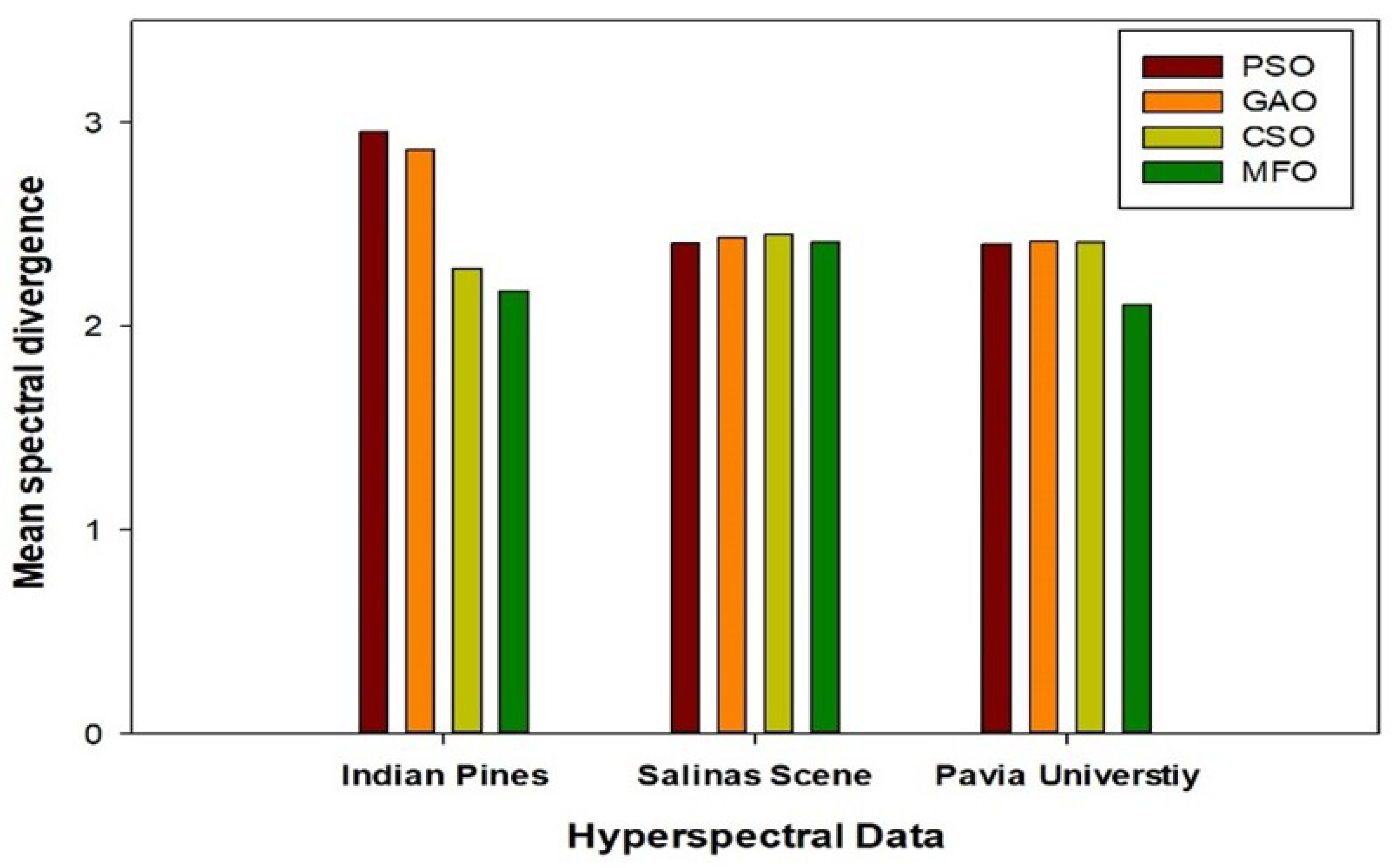
5.1. Comparative Analysis of State-of-the-Art Techniques with Respect to Overall and Average Accuracies
5.2. Computation Time
6. Conclusions
Author Contributions
Funding
Institutional Review Board Statement
Informed Consent Statement
Data Availability Statement
Conflicts of Interest
References
- Chang, C.I. Hyperspectral Imaging: Techniques for Spectral Detection And Classification; Springer Science & Business Media: Berlin/Heidelberg, Germany, 2003; Volume 1. [Google Scholar]
- Shahshahani, B.M.; Landgrebe, D.A. The effect of unlabeled samples in reducing the small sample size problem and mitigating the Hughes phenomenon. IEEE Trans. Geosci. Remote Sens. 1994, 32, 1087–1095. [Google Scholar] [CrossRef] [Green Version]
- McKeown, D.M.; Cochran, S.D.; Ford, S.J.; McGlone, J.C.; Shufelt, J.A.; Yocum, D.A. Fusion of HYDICE hyperspectral data with panchromatic imagery for cartographic feature extraction. IEEE Trans. Geosci. Remote Sens. 1999, 37, 1261–1277. [Google Scholar] [CrossRef]
- Liu, B.; Yu, X.; Zhang, P.; Yu, A.; Fu, Q.; Wei, X. Supervised deep feature extraction for hyperspectral image classification. IEEE Trans. Geosci. Remote Sens. 2017, 56, 1909–1921. [Google Scholar] [CrossRef]
- Damodaran, B.B.; Courty, N.; Lefèvre, S. Sparse Hilbert Schmidt independence criterion and surrogate-kernel-based feature selection for hyperspectral image classification. IEEE Trans. Geosci. Remote Sens. 2017, 55, 2385–2398. [Google Scholar] [CrossRef] [Green Version]
- Zebari, R.; Abdulazeez, A.; Zeebaree, D.; Zebari, D.; Saeed, J. A Comprehensive Review of Dimensionality Reduction Techniques for Feature Selection and Feature Extraction. J. Appl. Sci. Technol. Trends 2020, 1, 56–70. [Google Scholar] [CrossRef]
- Ho, Y.C.; Pepyne, D.L. Simple explanation of the no-free-lunch theorem and its implications. J. Optim. Theory Appl. 2002, 115, 549–570. [Google Scholar] [CrossRef]
- Wolpert, D.H.; Macready, W.G. No free lunch theorems for optimization. IEEE Trans. Evol. Comput. 1997, 1, 67–82. [Google Scholar] [CrossRef] [Green Version]
- Kennedy, J.; Eberhart, R. Particle swarm optimization. In Proceedings of the ICNN’95—International Conference on Neural Networks, Perth, WA, Australia, 27 November–1 December 1995; Volume 4, pp. 1942–1948. [Google Scholar]
- Chang, Y.L.; Fang, J.P.; Benediktsson, J.A.; Chang, L.; Ren, H.; Chen, K.S. Band selection for hyperspectral images based on parallel particle swarm optimization schemes. In Proceedings of the 2009 IEEE International Geoscience and Remote Sensing Symposium, Cape Town, South Africa, 12–17 July 2009; Volume 5, p. V-84. [Google Scholar]
- Grefenstette, J.J. Genetic algorithms and machine learning. In Proceedings of the Sixth Annual Conference on Computational Learning Theory, Santa Cruz, CA, USA, 26–28 July 1993; pp. 3–4. [Google Scholar]
- Moradi, M.H.; Abedini, M. A combination of genetic algorithm and particle swarm optimization for optimal DG location and sizing in distribution systems. Int. J. Electr. Power Energy Syst. 2012, 34, 66–74. [Google Scholar] [CrossRef]
- Yang, X.S.; Deb, S. Engineering optimization by cuckoo search. Int. J. Math. Model. Numer. Optim. 2010, 1, 330–343. [Google Scholar]
- Medjahed, S.A.; Saadi, T.A.; Benyettou, A.; Ouali, M. Binary cuckoo search algorithm for band selection in hyperspectral image classification. IAENG Int. J. Comput. Sci. 2015, 42, 183–191. [Google Scholar]
- Wang, G. A comparative study of cuckoo algorithm and ant colony algorithm in optimal path problems. MATEC Web Conf. EDP Sci. 2018, 232, 03003. [Google Scholar] [CrossRef] [Green Version]
- Li, Y.; Zhu, X.; Liu, J. An Improved Moth-Flame Optimization Algorithm for Engineering Problems. Symmetry 2020, 12, 1234. [Google Scholar] [CrossRef]
- Helmi, A.; Alenany, A. An enhanced Moth-flame optimization algorithm for permutation-based problems. Evol. Intell. 2020, 13, 741–764. [Google Scholar] [CrossRef]
- Mohamed, A.A.; Kamel, S.; Hassan, M.H.; Mosaad, M.I.; Aljohani, M. Optimal Power Flow Analysis Based on Hybrid Gradient-Based Optimizer with Moth–Flame Optimization Algorithm Considering Optimal Placement and Sizing of FACTS/Wind Power. Mathematics 2022, 10, 361. [Google Scholar] [CrossRef]
- Zhang, M.; Gong, M.; Chan, Y. Hyperspectral band selection based on multi-objective optimization with high information and low redundancy. Appl. Soft Comput. 2018, 70, 604–621. [Google Scholar] [CrossRef]
- Breiman, L. Random forests. Mach. Learn. 2001, 45, 5–32. [Google Scholar] [CrossRef] [Green Version]
- Zhang, M.L.; Zhou, Z.H. ML-KNN: A lazy learning approach to multi-label learning. Pattern Recognit. 2007, 40, 2038–2048. [Google Scholar] [CrossRef] [Green Version]
- Anand, R.; Veni, S.; Aravinth, J. Robust Classification Technique for Hyperspectral Images Based on 3D-Discrete Wavelet Transform. Remote Sens. 2021, 13, 1255. [Google Scholar] [CrossRef]
- Gualtieri, J.A.; Cromp, R.F. Support vector machines for hyperspectral remote sensing classification. In Proceedings of the 27th AIPR Workshop: Advances in Computer-Assisted Recognition, Washington, DC, USA, 14–16 October 1998; Volume 3584, pp. 221–232. [Google Scholar]
- Gualtieri, J.A.; Chettri, S.R.; Cromp, R.F.; Johnson, L.F. Support vector machine classifiers as applied to AVIRIS data. In Proceedings of the Eighth JPL Airborne Geoscience Workshop, Pasadena, CA, USA, 9–11 February 1999; pp. 217–227. [Google Scholar]
- Houshmand, B.; Gamba, P. Integration of High-Resolution Multispectral Imagery with Lidar and IFSAR Data for Urban Analysis Applications. Int. Arch. Photogramm. Remote Sens. 1999, 32, 111–117. [Google Scholar]
- Reshma, R.; Sowmya, V.; Soman, K.P. Dimensionality reduction using band selection technique for kernel based hyperspectral image classification. Procedia Comput. Sci. 2016, 93, 396–402. [Google Scholar] [CrossRef] [Green Version]
- Haridas, N.; Sowmya, V.; Soman, K.P. Gurls vs libsvm: Performance comparison of kernel methods for hyperspectral image classification. Indian J. Sci. Technol. 2015, 8, 1. [Google Scholar] [CrossRef] [Green Version]
- Xu, M.; Shi, J.; Chen, W.; Shen, J.; Gao, H.; Zhao, J. A band selection method for hyperspectral image based on particle swarm optimization algorithm with dynamic sub-swarms. J. Signal Process. Syst. 2018, 90, 1269–1279. [Google Scholar] [CrossRef]
- Sawant, S.; Manoharan, P. A hybrid optimization approach for hyperspectral band selection based on wind driven optimization and modified cuckoo search optimization. Multimed. Tools Appl. 2021, 80, 1725–1748. [Google Scholar] [CrossRef]
- Nagasubramanian, K.; Jones, S.; Sarkar, S.; Singh, A.K.; Singh, A.; Ganapathysubramanian, B. Hyperspectral band selection using genetic algorithm and support vector machines for early identification of charcoal rot disease in soybean stems. Plant Methods 2018, 14, 1–13. [Google Scholar] [CrossRef] [PubMed]
- Su, H.; Du, Q.; Chen, G.; Du, P. Optimised hyperspectral band selection using particle swarm optimization. IEEE J. Sel. Top. Appl. Earth Obs. Remote Sens. 2014, 7, 2659–2670. [Google Scholar] [CrossRef]
- Wen, G.; Zhang, C.; Lin, Z.; Xu, Y. Band selection based on genetic algorithms for classification of hyperspectral data. In Proceedings of the 2016 9th International Congress on Image and Signal Processing, BioMedical Engineering, and Informatics (CISP-BMEI), Datong, China, 15–17 October 2016; pp. 1173–1177. [Google Scholar]
- Shao, S. An improved cuckoo search-based adaptive band selection for hyperspectral image classification. Eur. J. Remote Sens. 2020, 53, 211–218. [Google Scholar] [CrossRef]
- Mirjalili, S. Moth-flame optimization algorithm: A novel nature-inspired heuristic paradigm. Knowl.-Based Syst. 2015, 89, 228–249. [Google Scholar] [CrossRef]


| Optimization Techniques | Airborne Hyperspectral Dataset | Non-Optimized Bands | Number of Non-Optimized Band |
|---|---|---|---|
| MFO | Indian Pines | [0, 1, 2, 4, 5, 6, 9, 57, 76, 79, 101, 102, 104, 141, 143, 191] | 16 |
| Salinas | [0, 1, 2, 3, 4, 5, 103, 104, 105, 106, 108, 146, 147] | 13 | |
| Pavia University | [0, 1, 2, 3, 6, 12, 15, 24, 26, 85, 94] | 11 | |
| PSO | Indian Pines | [0, 1, 2, 3, 4, 5, 6, 9, 57, 76, 79, 101, 102, 103, 104, 143, 144, 145, 191] | 19 |
| Salinas | [0, 1, 2, 3, 4, 16, 60, 79, 80, 105, 146, 155, 152] | 13 | |
| Pavia University | [0, 1, 3, 4, 5, 6, 11, 12, 24, 27, 44, 85, 94, 98, 101] | 15 | |
| GAO | Indian Pines | [0, 1, 2, 4, 5, 6, 7, 9, 16, 33, 41, 47, 57, 75, 82, 101, 104, 113, 124, 139, 144, 186, 181, 183] | 24 |
| Salinas | [0, 1, 2, 3, 4, 5, 6, 8, 31, 56, 102, 103, 106, 108, 144, 145, 157, 159, 161] | 19 | |
| Pavia University | [0, 1, 2, 3, 4, 5, 8, 12, 14, 15, 22, 26, 28, 36, 68, 86, 91, 101] | 18 | |
| CSO | Indian Pines | [0, 1, 4, 5, 7, 19, 41, 76, 77, 84, 89, 95, 100, 101, 102, 104, 143, 144, 174, 175, 184, 192] | 22 |
| Salinas | [0, 1, 2, 3, 4, 5, 8, 9, 21, 34, 46, 82, 86, 103, 104, 105, 107, 145, 146, 147] | 20 | |
| Pavia University | [0, 1, 2, 3, 4, 5, 6, 11, 14, 24, 26, 56, 57, 71, 84, 86, 94] | 17 |
| Indian Pines Hyperspectral Data | University of Pavia Hyperspectral Data | Salinas Scene Hyperspectral Data | |||||||||
|---|---|---|---|---|---|---|---|---|---|---|---|
| Class Name | Training Samples | Test Samples | Total Samples | Class Name | Training Samples | Test Samples | Total Samples | Class Name | Training Samples | Test Samples | Total Samples |
| Alfalfa | 9 | 36 | 45 | Asphalt | 1314 | 5256 | 6570 | Broccoli green weeds 1 | 419 | 1676 | 2095 |
| Corn-notill | 283 | 1130 | 1413 | Meadows | 3725 | 14,898.4 | 18,623 | Broccoli green weeds 2 | 737 | 2948 | 3685 |
| Corn-mintill | 169 | 674.4 | 843 | Bitumen | 420 | 1680 | 2100 | Fallow | 390 | 1558 | 1948 |
| Corn | 45 | 180 | 225 | Gravel | 619 | 2476 | 3095 | Fallow rough plow | 285 | 1140 | 1425 |
| Grass-pasture | 95 | 378.4 | 473 | Bare Soil | 286 | 1144 | 1430 | Fallow smooth | 559 | 2236 | 2795 |
| Grasstrees | 143 | 570.4 | 713 | Painted metal sheets | 1008 | 4030.4 | 5038 | Stubble | 817 | 3268 | 4085 |
| Grass- pasture- mowed | 6 | 24 | 30 | Self-Blocking Bricks | 269 | 1076 | 1345 | Celery | 703 | 2810 | 3513 |
| Hay- windrowed | 91 | 364 | 455 | Shadows | 729 | 2916 | 3645 | Grapes untrained | 2205 | 8820 | 11025 |
| Oats | 3 | 10.4 | 13 | Trees | 187 | 746.4 | 933 | Soil vineyard develop | 1231 | 4924 | 6155 |
| Soybean-notill | 206 | 822.4 | 1028 | Corn senesced green weeds | 659 | 2634 | 3293 | ||||
| Soybean-mintill | 484 | 1936 | 2420 | Lettuce romaine 4 wk | 199 | 794 | 993 | ||||
| Soybean-clean | 123 | 490.4 | 613 | Lettuce romaine 5 wk | 383 | 1530 | 1913 | ||||
| Wheat | 41 | 164 | 205 | Lettuce romaine 6 wk | 176 | 702 | 878 | ||||
| Woods | 259 | 1036 | 1295 | Lettuce romaine 7 wk | 207 | 826 | 1033 | ||||
| Buildings Grass Trees Drives | 78 | 312 | 390 | Vineyard untrained | 1482 | 5928 | 7410 | ||||
| Stone Steel Towers | 19 | 74.4 | 93 | Vineyard vertical trellis | 378 | 1510 | 1888 | ||||
| Class Names of Indian Pines Dataset | RF | KNN | SVM | |||||||||
|---|---|---|---|---|---|---|---|---|---|---|---|---|
| PSO | GAO | CSO | MFO | PSO | GAO | CSO | MFO | PSO | GAO | CS | MFO | |
| Alfalfa | 61.11 | 55.56 | 66.67 | 61.11 | 55.56 | 55.56 | 61.11 | 72.22 | 94.44 | 94.44 | 88.89 | 100 |
| Corn-notill | 76.81 | 77.88 | 78.05 | 76.46 | 70.09 | 68.85 | 70.80 | 69.91 | 80.35 | 80.71 | 81.77 | 80.18 |
| Corn-mintill | 63.20 | 56.97 | 61.42 | 63.20 | 60.53 | 58.46 | 59.94 | 60.53 | 81.01 | 81.90 | 82.20 | 81.31 |
| Corn | 37.78 | 33.33 | 34.44 | 36.67 | 37.78 | 41.11 | 50 | 37.78 | 82.22 | 86.67 | 81.11 | 82.22 |
| Grass-pasture | 88.36 | 95.24 | 93.12 | 91.53 | 92.06 | 92.59 | 92.59 | 92.06 | 96.30 | 96.83 | 96.83 | 96.85 |
| Grasstrees | 97.89 | 98.25 | 97.54 | 97.54 | 97.19 | 96.84 | 97.54 | 97.19 | 97.89 | 97.54 | 97.82 | 100 |
| Grass-pasture-mowed | 58.33 | 75 | 50 | 66.67 | 75 | 66.67 | 75 | 100 | 83.33 | 83.33 | 83.33 | 100 |
| Hay-windrowed | 99.45 | 100 | 99.45 | 100 | 98.35 | 97.80 | 98.90 | 100.55 | 100 | 99.45 | 99.45 | 100 |
| Oats | 100 | 60 | 40 | 60 | 80 | 60 | 80 | 100 | 100 | 100 | 100 | 100 |
| Soybean-notill | 76.89 | 76.64 | 77.86 | 78.35 | 80.78 | 80.78 | 82.24 | 80.78 | 85.16 | 84.43 | 81.75 | 84.18 |
| Soybean-mintill | 90.81 | 89.88 | 90.19 | 90.70 | 79.96 | 79.75 | 79.75 | 80.06 | 89.67 | 90.08 | 90.08 | 89.77 |
| Soybean-clean | 75.92 | 75.10 | 74.29 | 74.29 | 48.98 | 48.98 | 49.80 | 48.98 | 87.76 | 86.12 | 85.71 | 88.16 |
| Wheat | 97.56 | 97.56 | 97.56 | 98.78 | 95.12 | 93.90 | 96.34 | 95.12 | 98.78 | 97.56 | 98.78 | 100 |
| Woods | 98.26 | 97.30 | 96.91 | 97.68 | 93.44 | 94.21 | 93.44 | 93.44 | 96.72 | 97.10 | 97.10 | 96.72 |
| Buildings Grass Trees Drives | 62.18 | 58.97 | 61.54 | 58.33 | 39.10 | 34.62 | 38.46 | 39.10 | 78.21 | 73.72 | 76.92 | 78.21 |
| Stone Steel Towers | 89.19 | 89.19 | 89.19 | 89.19 | 91.89 | 89.19 | 91.89 | 91.89 | 86.49 | 91.89 | 86.49 | 86.49 |
| Class Name of University of Pavia Data | RF | KNN | SVM | |||||||||
|---|---|---|---|---|---|---|---|---|---|---|---|---|
| PSO | GAO | CSO | MFO | PSO | GAO | CSO | MFO | PSO | GAO | CS | MFO | |
| Asphalt | 95.81 | 96.84 | 95.81 | 96.12 | 91.48 | 91.36 | 91.40 | 95.81 | 95.81 | 95.74 | 91.48 | 96.69 |
| Meadows | 98.13 | 98.34 | 98.44 | 98.46 | 98.35 | 98.43 | 98.32 | 98.43 | 98.43 | 98.50 | 98.35 | 98.67 |
| Bitumen | 78.45 | 73.33 | 78.69 | 71.19 | 75.83 | 77.26 | 75.60 | 78.45 | 78.45 | 78.81 | 75.83 | 76.43 |
| Gravel | 96.93 | 94.10 | 97.25 | 94.18 | 89.10 | 89.34 | 89.26 | 96.93 | 96.93 | 97.50 | 89.10 | 94.10 |
| Bare Soil | 100 | 99.83 | 100 | 100 | 99.65 | 99.65 | 99.48 | 100 | 100 | 100 | 99.65 | 100 |
| Painted metal sheets | 92.31 | 88.68 | 91.36 | 86.55 | 76.77 | 77.57 | 76.43 | 92.31 | 92.31 | 91.56 | 76.77 | 86.90 |
| Self-Blocking Bricks | 86.80 | 76.21 | 86.62 | 77.70 | 88.66 | 88.10 | 87.36 | 86.80 | 86.80 | 86.43 | 88.66 | 86.80 |
| Shadows | 93.07 | 93.14 | 92.87 | 92.59 | 88.82 | 90.19 | 88.89 | 93.07 | 93.07 | 93.07 | 88.82 | 93.21 |
| Trees | 100 | 100 | 100 | 100 | 100 | 100 | 100 | 100 | 100 | 100 | 100 | 100 |
| Class Name of Salinas Scene Data | RF | KNN | SVM | |||||||||
|---|---|---|---|---|---|---|---|---|---|---|---|---|
| PSO | GAO | CSO | MFO | PSO | GAO | CSO | MFO | PSO | GAO | CSO | MFO | |
| Broccoli green weeds 1 | 99.16 | 99.18 | 99.18 | 99.18 | 98.69 | 98.69 | 98.69 | 98.69 | 99.14 | 98.01 | 98.17 | 99.52 |
| Broccoli green weeds 2 | 100 | 99.93 | 99.93 | 100 | 99.73 | 99.73 | 99.73 | 99.73 | 100 | 100 | 100 | 100 |
| Fallow | 100 | 99.87 | 100 | 99.87 | 100 | 100 | 100 | 100 | 100 | 100 | 100 | 100 |
| Fallow rough plow | 99.82 | 99.82 | 99.82 | 99.82 | 99.82 | 99.82 | 99.82 | 99.82 | 100 | 100 | 100 | 100 |
| Fallow smooth | 99.73 | 99.55 | 99.73 | 99.55 | 98.57 | 98.57 | 98.48 | 98.48 | 99.46 | 99.55 | 99.46 | 99.55 |
| Stubble | 99.94 | 98.86 | 98.17 | 98.41 | 99.76 | 99.76 | 99.76 | 99.76 | 98.12 | 99.87 | 99.13 | 99.94 |
| Celery | 98.32 | 99.71 | 99.64 | 99.72 | 99.36 | 99.29 | 99.36 | 99.36 | 99.72 | 99.72 | 99.72 | 99.72 |
| Grapes untrained | 93.40 | 93.58 | 93.56 | 93.58 | 85.78 | 85.60 | 85.56 | 85.78 | 90.77 | 90.86 | 90.77 | 91.02 |
| Soil vineyard develop | 99.96 | 100 | 99.96 | 99.96 | 99.59 | 99.63 | 99.63 | 99.63 | 99.92 | 99.92 | 99.92 | 99.92 |
| Corn senesced green weeds | 98.48 | 98.86 | 98.25 | 98.24 | 94.38 | 94.31 | 94.46 | 94.31 | 98.71 | 98.48 | 98.63 | 98.63 |
| Lettuce romaine 4 wk | 98.49 | 99.50 | 98.74 | 98.99 | 97.98 | 97.98 | 97.98 | 97.98 | 99.24 | 98.49 | 98.74 | 98.49 |
| Lettuce romaine 5 wk | 100 | 100 | 100 | 100 | 99.87 | 99.87 | 100 | 99.87 | 100 | 100 | 100 | 100 |
| Lettuce romaine 6 wk | 98.01 | 98.01 | 98.01 | 98.58 | 97.72 | 97.72 | 97.72 | 97.72 | 99.43 | 99.43 | 99.43 | 99.43 |
| Lettuce romaine 7 wk | 98.55 | 98.31 | 98.31 | 97.82 | 95.40 | 95.40 | 95.40 | 95.40 | 98.14 | 97.69 | 96.13 | 98.79 |
| Vineyard untrained | 78.58 | 78.37 | 77.63 | 77.67 | 69.80 | 68.93 | 69.47 | 69.43 | 71.29 | 70.72 | 70.38 | 70.82 |
| Vineyard vertical trellis | 98.94 | 98.94 | 98.94 | 98.94 | 98.54 | 98.41 | 98.41 | 98.41 | 99.07 | 98.94 | 99.07 | 98.94 |
| Class Name of Indian Pines Data | RF | KNN | SVM | |||||||||
|---|---|---|---|---|---|---|---|---|---|---|---|---|
| PSO | GA | CS | MFO | PSO | GA | CS | MFO | PSO | GA | CS | MFO | |
| Overall Accuracy | 83.68 | 83.02 | 83.41 | 83.54 | 77.32 | 76.80 | 77.88 | 77.51 | 88.90 | 88.93 | 88.78 | 88.98 |
| Average Accuracy | 79.61 | 77.30 | 75.51 | 77.18 | 74.74 | 72.46 | 76.11 | 77.68 | 89.90 | 90.11 | 89.27 | 91.37 |
| Kappa Coefficient | 0.81 | 0.81 | 0.81 | 0.81 | 0.74 | 0.74 | 0.75 | 0.75 | 0.87 | 0.88 | 0.87 | 0.88 |
| Class Name of University of Pavia Data | RF | KNN | SVM | |||||||||
|---|---|---|---|---|---|---|---|---|---|---|---|---|
| PSO | GA | CS | MFO | PSO | GA | CS | MFO | PSO | GA | CS | MFO | |
| Overall Accuracy | 93.98 | 94.38 | 93.99 | 93.98 | 91.94 | 92.24 | 91.84 | 94.62 | 95.48 | 95.46 | 95.39 | 96.94 |
| Average Accuracy | 90.75 | 91.16 | 90.64 | 90.75 | 89.85 | 90.21 | 89.64 | 92.49 | 93.53 | 93.51 | 93.45 | 94.85 |
| Kappa Coefficient | 0.92 | 0.93 | 0.92 | 0.92 | 0.89 | 0.90 | 0.89 | 0.93 | 0.94 | 0.94 | 0.94 | 0.89 |
| Class Name of Salinas Scene Data | RF | KNN | SVM | |||||||||
|---|---|---|---|---|---|---|---|---|---|---|---|---|
| PSO | GA | CS | MFO | PSO | GA | CS | MFO | PSO | GA | CS | MFO | |
| Overall Accuracy | 95.45 | 95.49 | 95.34 | 95.39 | 92.16 | 91.99 | 92.07 | 92.10 | 93.95 | 93.82 | 93.87 | 93.92 |
| Average Accuracy | 97.71 | 97.77 | 97.65 | 97.70 | 95.94 | 95.86 | 95.90 | 95.90 | 97.24 | 97.15 | 97.15 | 97.17 |
| Kappa Coefficient | 0.95 | 0.95 | 0.95 | 0.95 | 0.91 | 0.91 | 0.91 | 0.91 | 0.93 | 0.93 | 0.93 | 0.93 |
| Optimization Techniques | Random Forest | K-Nearest Neighbor | Support Vector Machine | |
|---|---|---|---|---|
| Indian Pines | MFO | 165 | 184 | 206 |
| CSO | 188 | 172 | 195 | |
| GAO | 348 | 647 | 647 | |
| PSO | 557 | 628 | 722 | |
| University of Pavia | MFO | 714 | 768 | 802 |
| CSO | 644 | 704 | 785 | |
| GAO | 984 | 1084 | 1102 | |
| PSO | 1023 | 1069 | 1248 | |
| Salinas Scene | MFO | 897 | 831 | 1046 |
| CSO | 974 | 1003 | 1086 | |
| GAO | 1142 | 1340 | 1424 | |
| PSO | 1267 | 2018 | 2123 | |
Publisher’s Note: MDPI stays neutral with regard to jurisdictional claims in published maps and institutional affiliations. |
© 2022 by the authors. Licensee MDPI, Basel, Switzerland. This article is an open access article distributed under the terms and conditions of the Creative Commons Attribution (CC BY) license (https://creativecommons.org/licenses/by/4.0/).
Share and Cite
Anand, R.; Samiaappan, S.; Veni, S.; Worch, E.; Zhou, M. Airborne Hyperspectral Imagery for Band Selection Using Moth–Flame Metaheuristic Optimization. J. Imaging 2022, 8, 126. https://doi.org/10.3390/jimaging8050126
Anand R, Samiaappan S, Veni S, Worch E, Zhou M. Airborne Hyperspectral Imagery for Band Selection Using Moth–Flame Metaheuristic Optimization. Journal of Imaging. 2022; 8(5):126. https://doi.org/10.3390/jimaging8050126
Chicago/Turabian StyleAnand, Raju, Sathishkumar Samiaappan, Shanmugham Veni, Ethan Worch, and Meilun Zhou. 2022. "Airborne Hyperspectral Imagery for Band Selection Using Moth–Flame Metaheuristic Optimization" Journal of Imaging 8, no. 5: 126. https://doi.org/10.3390/jimaging8050126
APA StyleAnand, R., Samiaappan, S., Veni, S., Worch, E., & Zhou, M. (2022). Airborne Hyperspectral Imagery for Band Selection Using Moth–Flame Metaheuristic Optimization. Journal of Imaging, 8(5), 126. https://doi.org/10.3390/jimaging8050126