
Comparison of 2D Optical Imaging and 3D Microtomography Shape Measurements of a Coastal Bioclastic Calcareous Sand

 ,
,  ,
,  , and
, and
Abstract
:1. Introduction
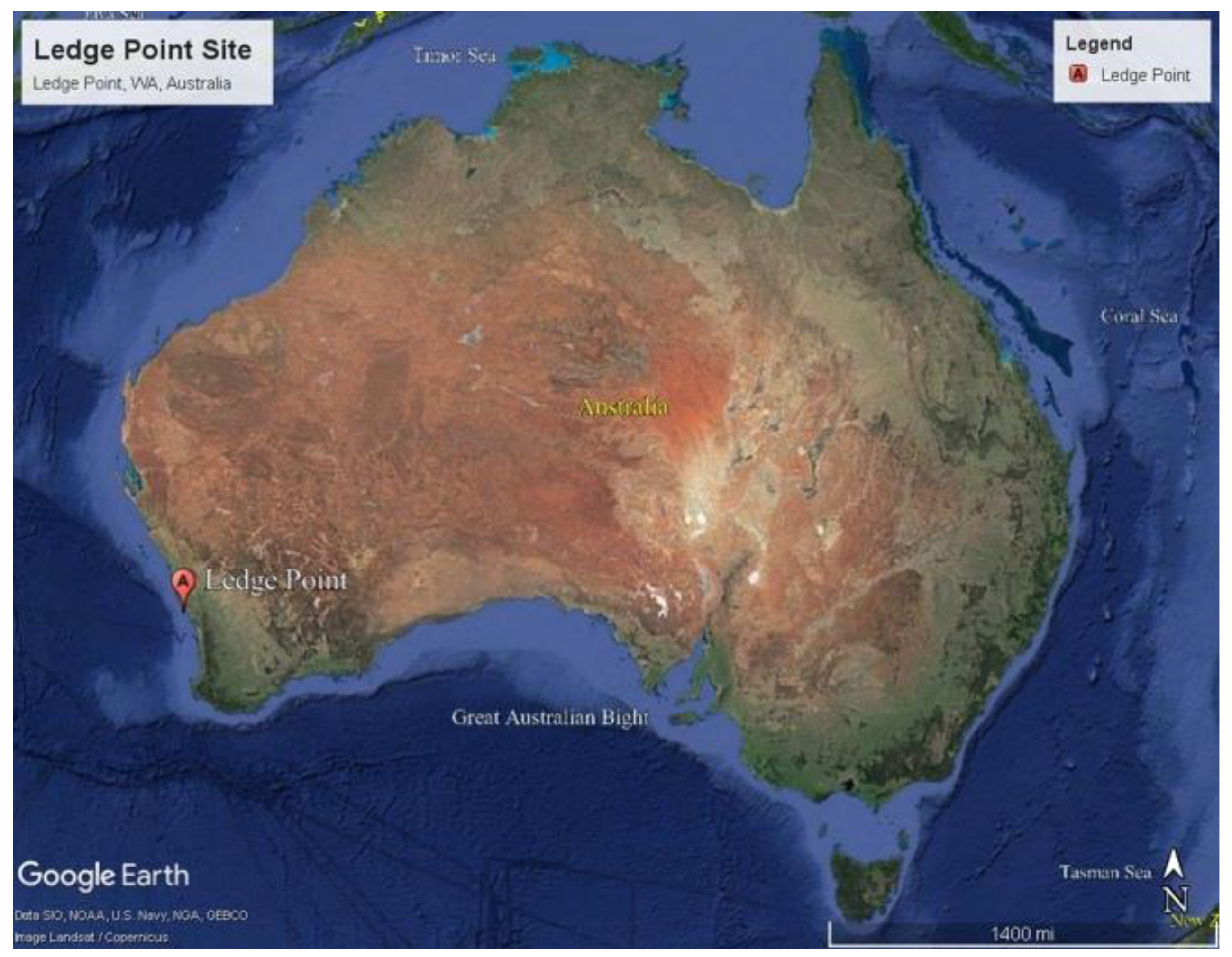
2. Sand in Study
3. Microscopy Techniques
3.1. Dynamic Image Analysis (DIA)
3.2. X-ray Microtomography
3.3. Three-Dimensional Watershed Segmentation
4. Shape Parameters
4.1. 2D Shape Parameters
4.2. 3D Shape Parameters
5. Results
5.1. Particle Size Distribution
5.2. Shape Parameter Variation with Size
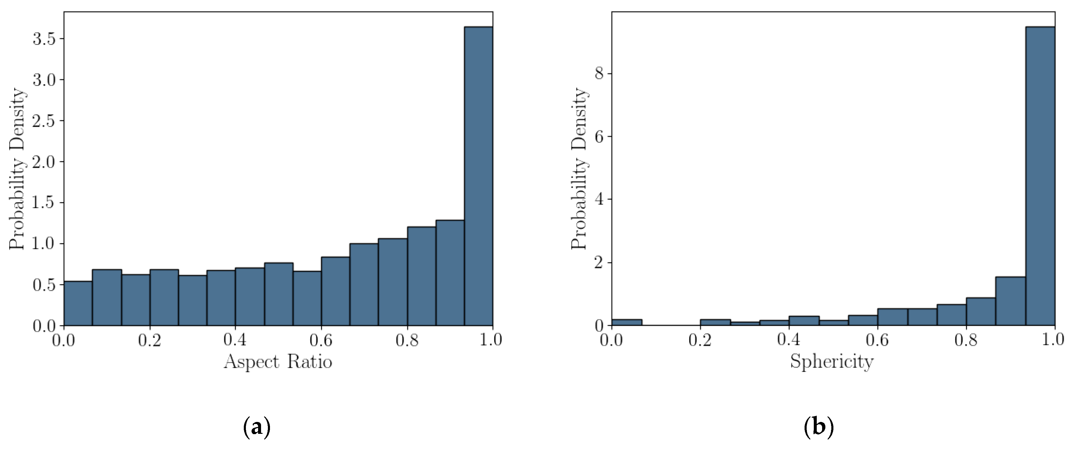
5.3. Statistics of Particle Shape Parameter
5.4. Correlation of Particle Shape Parameters
6. Discussion
7. Practical Significance of This Study
8. Conclusions
- For this calcareous sand, 2D DIA correlates better to the traditional sieve analysis than 3D μCT, as shown in Figure 4. The μCT analysis underestimates the number of fine sand grains below 0.2 mm relative to the sieve test. This is possibly due to the watershed algorithm used for segmenting the sand, which digitally removes smaller grains. Alternatively, it may be due to sampling error arising from the limited imaging volume captured by the μCT device compared with the 2D DIA technique.
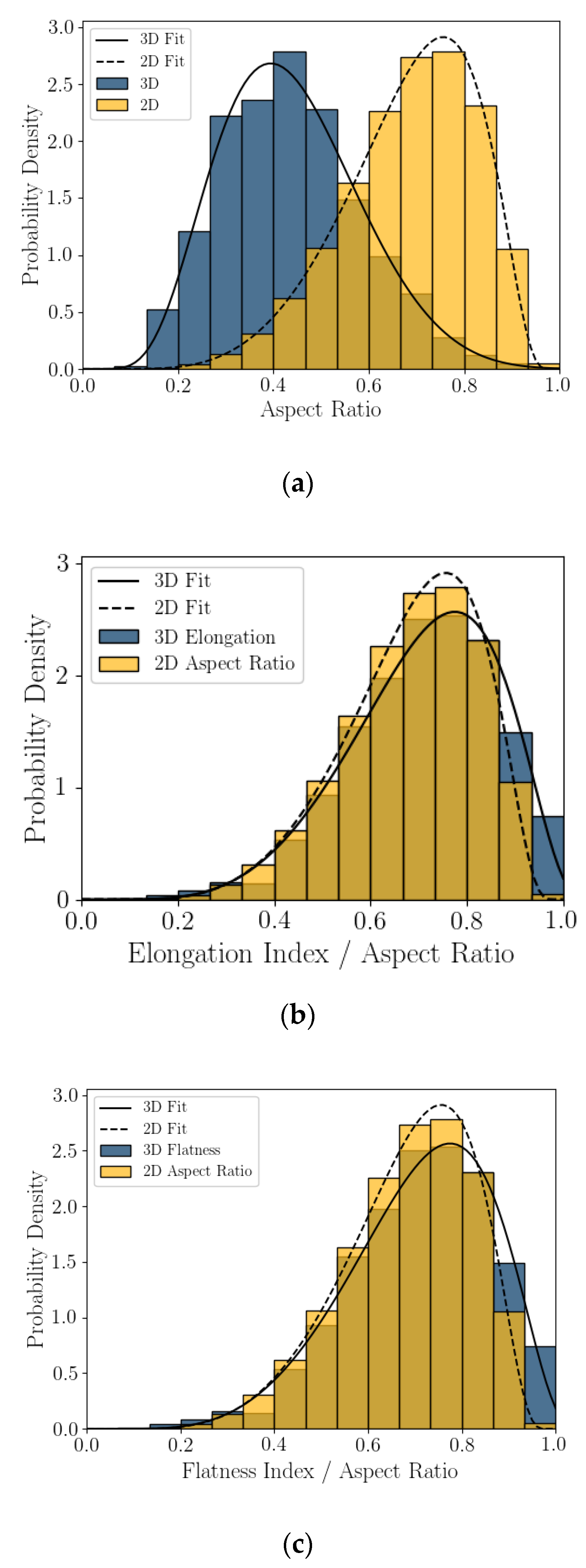
- The 2D DIA mean particle shape parameters aspect ratio, sphericity, and convexity with size were significantly larger (dependent on grain size) than those from 3D μCT (Figure 5).
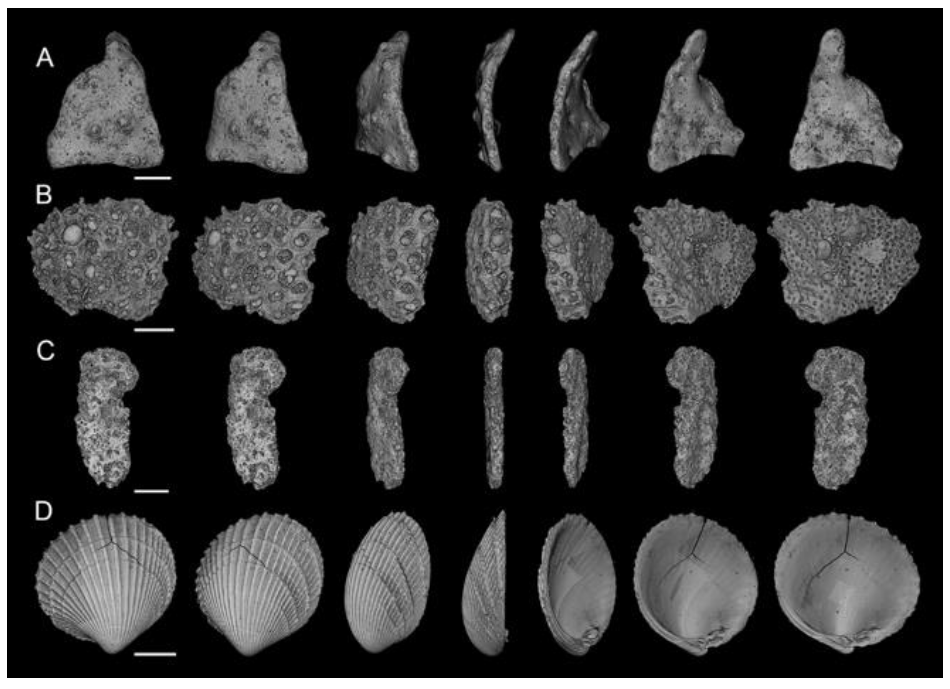
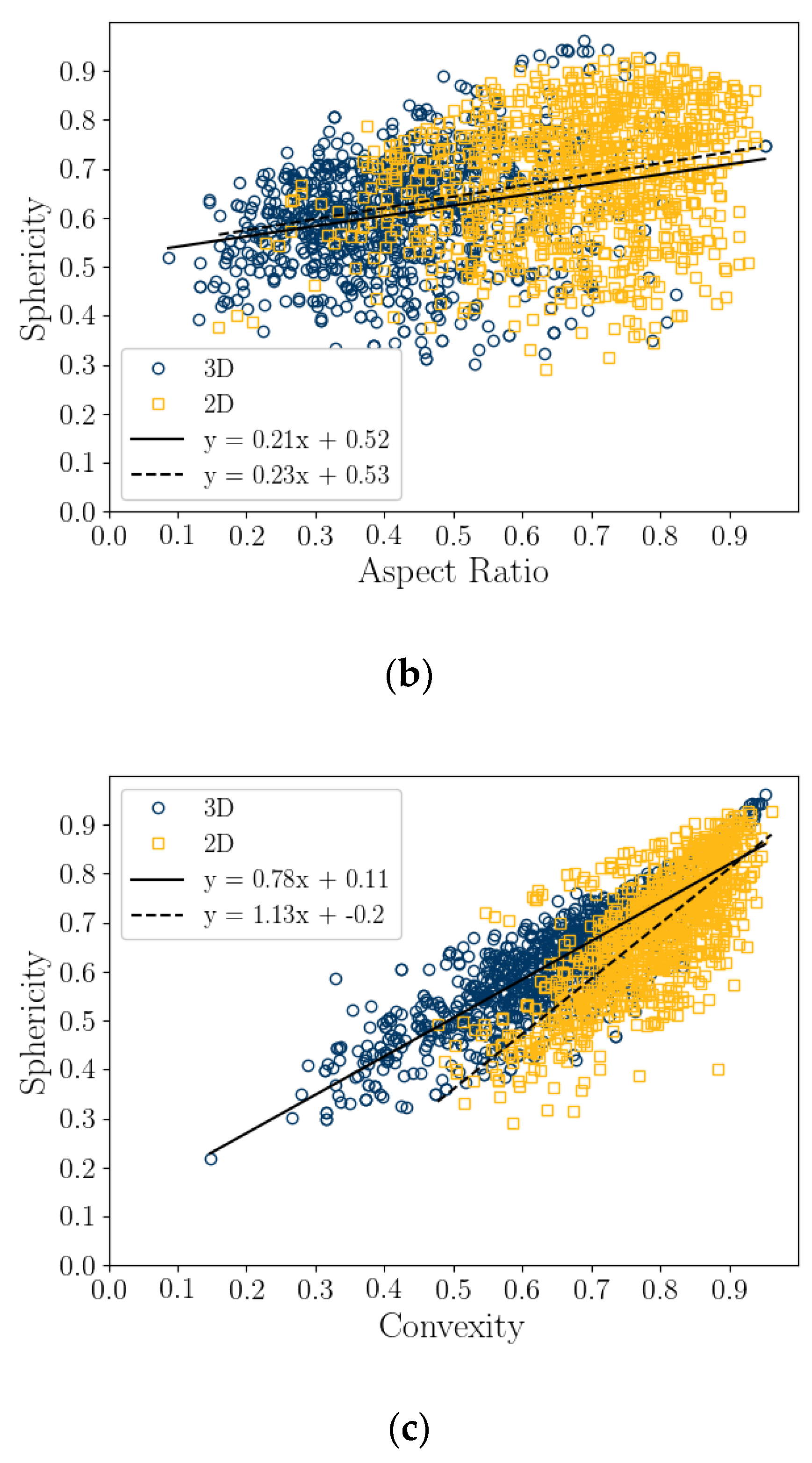
- The 3D μCT imaging technique is a more accurate method for measuring particle shape parameters of a bioclastic calcareous sand. When measured in 3D, the grains had a lower aspect ratio, AR3D vs. AR2D; had a lower convexity, Cx3D vs. Cx2D; and had a lower sphericity, S3D vs. S2D, as shown in Figure 6 and Figure 7. This agrees with the visual assessment of the randomly selected grains (Figure 2).
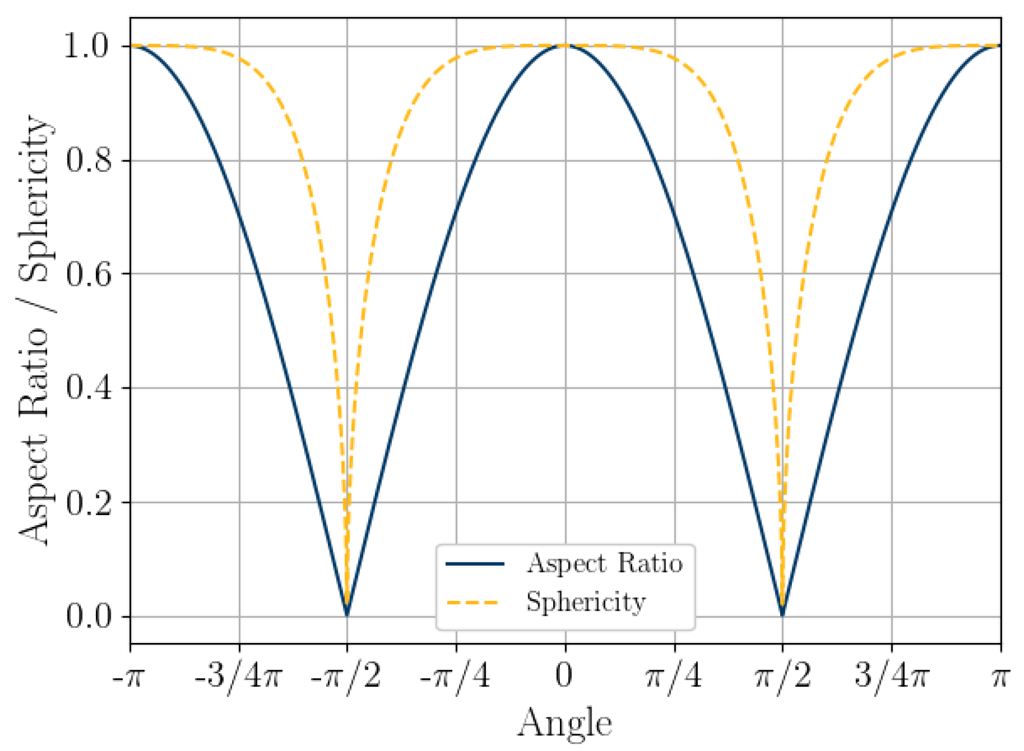
- Sphericity (S2D and S3D) is correlated with convexity (Cx2D and Cx3D), aspect ratio (AR2D and AR3D), elongation index (EI), and flatness index (FI) (Figure 8 and Figure 9). This is likely due to the biogenic nature of the soil in the case of 3D measurements and the imaging method in 2D measurements.
Author Contributions
Funding
Institutional Review Board Statement
Informed Consent Statement
Data Availability Statement
Acknowledgments
Conflicts of Interest
List of Notations
| A | Particle area |
| As | Surface area of a particle |
| A | Half the minimum Feret dimension |
| B | Half the maximum Feret dimension |
| Ac | Area of the convex hull |
| AR2D | Two-dimensional (2D) aspect ratio |
| AR3D | Three-dimensional (3D) aspect ratio |
| ARdisc | Aspect ratio of the project area of a disc rotated about a single axis at angle, θ |
| Cx2D | 2D convexity |
| Cx3D | Three-dimensional (3D) convexity |
| dEQPC | Diameter of an equivalent circle having an area equal to that of the projected particle area |
| dEQPC-disc | Diameter of an equivalent circle having an area equal to that of the projected disc rotating about its vertical axis |
| dESD | Diameter of an equivalent sphere having the same volume as the particle |
| dFlength | In 3D, the longest Feret dimensions |
| dFmax | Maximum Feret dimension |
| dFmin | Minimum Feret dimension |
| dFthickness | In 3D, the shortest Feret dimensions |
| dFwidth | In 3D, the intermediate Feret dimensions |
| EI | Elongation index |
| emax | Maximum void ratio |
| emin | Minimum void ratio |
| FI | Flatness index |
| P | Perimeter |
| Sa | Particle surface area |
| S2D | 2D sphericity |
| S3D | 3D sphericity |
| Sdisc | Sphericity of the project area of a disc rotated about a single axis at angle, θ |
| Vc | Volume of the convex hull |
| Vfill | Volume of the infilled particle, for porous and hollow particles |
| γ | Fitting parameter of the Johnson SB distribution |
| δ | Fitting parameter of the Johnson SB distribution |
| θ | Angle of rotation |
| λ | Scale parameter of the Johnson SB distribution |
| ξ | Location parameter of Johnson SB distribution |
References
- Altuhafi, F.N.; Coop, M.R.; Georgiannou, V.N. Effect of particle shape on the mechanical properties of natural sands. J. Geotech. Geoenviron. Eng. ASCE 2016, 142, 145. [Google Scholar] [CrossRef]
- Cavarretta, I.; Coop, M.; O'Sullivan, C. The influence of particle characteristics on the behaviour of coarse grained soils. Géotechnique 2010, 60, 413–423. [Google Scholar] [CrossRef] [Green Version]
- Cho, G.-C.; Dodds, J.; Santamarina, J.C. Particle Shape Effects on Packing Density, Stiffness, and Strength: Natural and Crushed Sands. J. Geotech. Geoenviron. Eng. 2006, 132, 591–602. [Google Scholar] [CrossRef] [Green Version]
- Guida, G.; Sebastiani, D.; Casini, F.; Miliziano, S. Grain morphology and strength dilatancy of sands. Géotechnique Lett. 2019, 9, 245–253. [Google Scholar] [CrossRef]
- Zheng, J.; Hryciw, R.D. Soil Particle Size and Shape Distributions by Stereophotography and Image Analysis. Geotech. Test. J. 2017, 40, 317–328. [Google Scholar] [CrossRef]
- Altuhafi, F.; O’Sullivan, C.; Cavarretta, I. Analysis of an Image-Based Method to Quantify the Size and Shape of Sand Particles. J. Geotech. Geoenviron. Eng. 2013, 139, 1290–1307. [Google Scholar] [CrossRef]
- Li, L.; Iskander, M. Evaluation of Dynamic Image Analysis for Characterizing Granular Soils. Geotech. Test. J. 2019, 43, 1149–1173. [Google Scholar] [CrossRef]
- Wei, H.; Zhao, T.; Meng, Q.; Wang, X.; Zhang, B. Quantifying the Morphology of Calcareous Sands by Dynamic Image Analysis. Int. J. Géoméch. 2020, 20, 04020020. [Google Scholar] [CrossRef]
- White, D.J. PSD measurement using the single particle optical sizing (SPOS) method. Géotechnique 2003, 53, 317–326. [Google Scholar] [CrossRef]
- Cnudde, V.; Boone, M.N. High-resolution X-ray computed tomography in geosciences: A review of the current technology and applications. Earth-Sci. Rev. 2013, 123, 1–17. [Google Scholar] [CrossRef] [Green Version]
- Fonseca, J.; O’Sullivan, C.; Coop, M.R.; Lee, P.D. Non-invasive characterization of particle morphology of natural sands. Soils Found. 2012, 52, 712–722. [Google Scholar] [CrossRef]
- Hall, S.; Bornert, M.; Desrues, J.; Pannier, Y.; Lenoir, N.; Viggiani, G.; Bésuelle, P. Discrete and continuum analysis of localised deformation in sand using X-ray μCT and volumetric digital image correlation. Géotechnique 2010, 60, 315–322. [Google Scholar] [CrossRef]
- Beemer, R.D.; Bandini-Maeder, A.N.; Shaw, J.; Lebrec, U.; Cassidy, M.J. The granular structure of two marine carbonate sediments. In Proceedings of the 37th International Conference on Ocean, Offshore & Arctic Engineering, Madrid, Spain, 17–22 June 2018. [Google Scholar]
- Kong, D.; Fonseca, J. Quantification of the morphology of shelly carbonate sands using 3D images. Géotechnique 2018, 68, 249–261. [Google Scholar] [CrossRef] [Green Version]
- Li, L.; Beemer, R.D.; Iskander, M. Granulometry of Two Marine Calcareous Sands. J. Geotech. Geoenviron. Eng. 2021, 147, 04020171. [Google Scholar] [CrossRef]
- Beemer, R.D.; Bandini-Maeder, A.N.; Shaw, J.; Cassidy, M.J. Volumetric Particle Size Distribution and Variable Granular Density Soils. Geotech. Test. J. 2019, 43. [Google Scholar] [CrossRef]
- Beemer, R.D.; Sadekov, A.; Lebrec, U.; Shaw, J.; Bandini-Maeder, A.; Cassidy, M.J. Impact of Biology on Particle Crushing in Offshore Calcareous Sediments. In Geo-Congress 2019: Geotechnical Materials, Modeling, and Testing; ASCE: Philadelphia, PA, USA, 2019. [Google Scholar]
- Demars, K.R. Unique Engineering Properties and Compression Behavior of Deep-Sea Calcareous Sediments. In Geotechnical Properties, Behavior, and Performance of Calcareous Soils; ASTM STP 777; Demars, K., Chaney, R., Eds.; ASTM: Fort Lauderdale, FL, USA, 2009; pp. 97–112. [Google Scholar] [CrossRef]
- Golightly, C.; Hyde, A.F.L. Some fundamental properties of carbonate sands. In Engineering for Calcareous Sediments; Jewell, R.J., Andrews, D.C., Eds.; Balkema: Perth, Australia, 1988; pp. 69–78. [Google Scholar]
- Semple, R.M. Mechanical properties of carbonate soils. In Engineering for Calcareous Sediments; Jewell, R.J., Andrews, D.C., Eds.; Balkema: Perth, Australia, 1988; pp. 807–836. [Google Scholar]
- Khorshid, M.S.E.D. Development of geotechnical experience on the North West Shelf. Trans. Inst. Eng. Australia. 1990, 32, 11–21. [Google Scholar]
- Li, L.; Sun, Q.; Iskander, M. Efficacy of 3D dynamic image analysis for characterising the morphology of natural sands. Géotechnique 2022, 1–14. [Google Scholar] [CrossRef]
- Li, L.; Iskander, M. Comparison of 2D and 3D dynamic image analysis for characterization of natural sands. Eng. Geol. 2021, 290, 106052. [Google Scholar] [CrossRef]
- Rorato, R.; Arroyo, M.; Andò, E.; Gens, A. Sphericity measures of sand grains. Eng. Geol. 2019, 254, 43–53. [Google Scholar] [CrossRef]
- Sharma, S.S. Characterisation of cyclic behaviour of calcite cemented calcareous soils. Ph.D. Thesis, University of Western Australia, Perth, Australia, 2004. [Google Scholar]
- Leonti, A.; Fonseca, J.; Valova, I.; Beemer, R.; Cannistraro, D.; Pilskaln, C.; Deflorio, D.; Kelly, G. Optimized 3D Segmentation Algorithm for Shelly Sand Images. In proceeding of the 6th World Congress on Electrical Engineering and Computer Systems and Science (EECSS'20), Virtual Conference, 13–15 August 2020. [Google Scholar]
- Otsu, N. A Threshold selection method from gray-level histogram. IEEE Trans. Syst. Man Cybern. 1979, 9, 62–66. [Google Scholar] [CrossRef] [Green Version]
- ISO 9276–6. Representation of Results of Particle Size Analysis—Part 6: Descriptive and Quantitative Representation of Particle Shape and Morphology; ISO: Geneva, Switzerland, 2008. [Google Scholar]
- ASTM. Standard Practice for Characterization of Particles; ASTM F1877; ASTM: West Conshohocken, PA, USA, 2016. [Google Scholar]
- Krumbein, W.C. Measurement and Geological Significance of Shape and Roundness of Sedimentary Particles. J. Sediment. Res. 1941, 11. [Google Scholar] [CrossRef]
- Zingg, T. Beitrag zur Schotteranalyse. Ph.D. Thesis, ETH Zurich, Zürich, Switzerland, 1935. (In German). [Google Scholar]
- Wadell, H. Volume, Shape, and Roundness of Quartz Particles. J. Geol. 1935, 43, 250–280. [Google Scholar] [CrossRef]
- ASTM. ASTM D6913 Standard Test Methods for Particle-Size Distribution (Gradation) of Soils Using Sieve Analysis; ASTM International: West Conshohocken, PA, USA, 2017. [Google Scholar]
- Johnson, N.L. Systems of Frequency Curves Generated by Methods of Translation. Biometrika 1949, 36, 29. [Google Scholar] [CrossRef]
- Ching, J.; Phoon, K.-K. Constructing multivariate distributions for soil parameters. In Risk and Reliability in Geotechnical Engineering; Taylor & Francis: Boca Raton, FL, USA, 2015; pp. 3–76. [Google Scholar]
- Virtanen, P.; Gommers, R.; Oliphant, T.E.; Haberland, M.; Reddy, T.; Cournapeau, D.; Burovski, E.; Peterson, P.; Weckesser, W.; Bright, J.; et al. SciPy 1.0: Fundamental Algorithms for Scientific Computing in Python. Nat. Methods 2020, 17, 261–272. [Google Scholar] [CrossRef] [PubMed] [Green Version]
- Ramanujan, S. Modular Equations and Approximations to π. Q. J. Math. 1914, 45, 350–372. [Google Scholar]
- Dutt, R.; Ingram, W. Discussion of ‘Classification of Marine Sediments. J. Geotech. Eng. 1990, 116, 1288–1289. [Google Scholar] [CrossRef]
- Clark, A.R.; Walker, B.F. A proposed scheme for the classification and nomemclature for use in the engineering description on Middle Eastern sedimentary rocks. Géotechnique 1977, 27, 93–99. [Google Scholar] [CrossRef]
- Murff, J.D. Pile Capacity in Calcareous Sands: State if the Art. J. Geotech. Eng. 1987, 113, 490–507. [Google Scholar] [CrossRef]
- Watson, P.; Bransby, F.; Delimi, Z.L.; Erbrich, C.; Finnie, I.; Krisdani, H.; Meecham, C.; Randolph, M.; Rattley, M.; Silva, M.; et al. Foundation Design in Offshore Carbonate Sediments–Building on Knowledge to Address Future Challenges. In Proceedings of the from Research to Applied Geotechnics: Invited Lectures of the XVI Pan-American Conference on Soil Mechanics and Geotechnical Engineering (XVI PCSMGE), Cancun, Mexico, 17–20 November 2019. [Google Scholar]


| Name | Location | Water Depth m | D50 µm | CaCO3 % | emin | emax |
|---|---|---|---|---|---|---|
| Ledge Point | Ledge Point, WA, Australia | 0 | 270 | 91 | 0.90 | 1.21 |
| DIA | Formula/Explanation | µCT | Formula/Explanation | |||||
|---|---|---|---|---|---|---|---|---|
| Size Descriptors | EQPC (dEQPC) | Diameter of circle with equivalent particle area |  | ESD (dESD) | Diameter of sphere with equivalent particle volume |  | ||
| Feret-max (dFmax) | Maximum dimension of a particle, aka. Maximum Feret diameter | 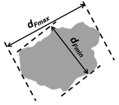 | dFlength | Longest axis |  | |||
| Feret-min (dFmin) | Minimum dimension of a particle, aka. Minimum Feret diameter | dFwidth | Intermediate axis | |||||
| dFthickness | Shortest axis | |||||||
| Shape Descriptors | Aspect ratio (AR2D) | Ratio of Feret-min to Feret-max | — | AR3D | Ratio of shortest to longest axes | |||
| Flatness index (FI) | Ratio of shortest to intermediate axes | |||||||
| Elongation index (EI) | Ratio of intermediate to longest axes | |||||||
| Sphericity (S2D) | Ratio of the perimeter of a circle with equivalent area to the real particle perimeter |  | Sphericity (S3D) | Ratio of the surface area of a volume equivalent sphere to the real particle surface area |  | |||
| Convexity (Cx2D) | Ratio between the particle area and the area of its convex hull |  | Convexity (Cx3D) | The ratio of the particle volume and the volume of its convex hull |  | |||
| Sieve Size (mm) |
|---|
| 4.75 |
| 2.36 |
| 1.18 |
| 0.60 |
| 0.425 |
| 0.30 |
| 0.180 |
| 0.15 |
| 0.106 |
| 0.075 |
| 0.0 |
| Sphericity (S2D or S3D) | Convexity (Cx2D or Cx3D) | Aspect Ratio (AR2D or AR3D) | Flatness (FI) | Elongation (EI) | |
|---|---|---|---|---|---|
| 2D Johnson Bounded Distribution | |||||
| γ: | −0.8053 | −2.2276 | −1.1976 | — | — |
| δ: | 1.2594 | 1.6607 | 1.3674 | — | — |
| ξ: | 0.1809 | 0.0999 | 0.0294 | — | — |
| λ: | 0.7935 | 0.8872 | 0.9557 | — | — |
| 3D Johnson Bounded Distribution | |||||
| γ: | −2.102e6 | −4.3393 | 1.3406 | −0.0989 | −1.0627 |
| δ: | 1.133e7 | 4.9303 | 1.8807 | 1.0247 | 1.4269 |
| ξ: | −2.92136 | −1.5005 | 0.0001 | 0.1603 | 0.0095 |
| λ: | 5.348e6 | 3.0300 | 1.2916 | 0.8958 | 1.0573 |
| EQPC | Aspect Ratio | Convexity | Sphericity | ||
|---|---|---|---|---|---|
| (dEQPC) | (AR2D) | (Cx2D) | (S2D) | ||
| EQPC | (dEQPC) | 1 | — | — | — |
| Aspect ratio | (AR2D) | −0.12 | 1 | — | — |
| Convexity | (Cx2D) | 0.35 | 0.02 | 1 | — |
| Sphericity | (S2D) | −0.06 | 0.24 | 0.77 | 1 |
| ESD | Aspect Ratio | Elongation | Flatness | Convexity | Sphericity | ||
|---|---|---|---|---|---|---|---|
| dESD | (AR3D) | EI | FI | (Cx3D) | (S3D) | ||
| ESD | (dESD) | 1 | — | — | — | — | — |
| Aspect ratio | (AR3D) | −0.07 | 1 | — | — | — | — |
| Elongation | EI | 0.03 | 0.47 | 1 | — | — | — |
| Flatness | FI | −0.10 | 0.72 | −0.25 | 1 | — | — |
| Convexity | (Cx3D) | −0.23 | 0.08 | 0.01 | 0.09 | 1 | — |
| Sphericity | (S3D) | −0.48 | 0.26 | 0.02 | 0.28 | 0.85 | 1 |
Publisher’s Note: MDPI stays neutral with regard to jurisdictional claims in published maps and institutional affiliations. |
© 2022 by the authors. Licensee MDPI, Basel, Switzerland. This article is an open access article distributed under the terms and conditions of the Creative Commons Attribution (CC BY) license (https://creativecommons.org/licenses/by/4.0/).
Share and Cite
Beemer, R.D.; Li, L.; Leonti, A.; Shaw, J.; Fonseca, J.; Valova, I.; Iskander, M.; Pilskaln, C.H. Comparison of 2D Optical Imaging and 3D Microtomography Shape Measurements of a Coastal Bioclastic Calcareous Sand. J. Imaging 2022, 8, 72. https://doi.org/10.3390/jimaging8030072
Beemer RD, Li L, Leonti A, Shaw J, Fonseca J, Valova I, Iskander M, Pilskaln CH. Comparison of 2D Optical Imaging and 3D Microtomography Shape Measurements of a Coastal Bioclastic Calcareous Sand. Journal of Imaging. 2022; 8(3):72. https://doi.org/10.3390/jimaging8030072
Chicago/Turabian StyleBeemer, Ryan D., Linzhu Li, Antonio Leonti, Jeremy Shaw, Joana Fonseca, Iren Valova, Magued Iskander, and Cynthia H. Pilskaln. 2022. "Comparison of 2D Optical Imaging and 3D Microtomography Shape Measurements of a Coastal Bioclastic Calcareous Sand" Journal of Imaging 8, no. 3: 72. https://doi.org/10.3390/jimaging8030072
APA StyleBeemer, R. D., Li, L., Leonti, A., Shaw, J., Fonseca, J., Valova, I., Iskander, M., & Pilskaln, C. H. (2022). Comparison of 2D Optical Imaging and 3D Microtomography Shape Measurements of a Coastal Bioclastic Calcareous Sand. Journal of Imaging, 8(3), 72. https://doi.org/10.3390/jimaging8030072