1. Introduction
In parallel with developments in the field of image capture technologies, data storage is becoming a significant issue encountered by computer and mobile users. Many encoding methods for image data storage have been developed, which can be divided into lossy and lossless methods. Approaches using various techniques to compress data for storage without losing any bits of information in the original image (often captured by a camera or sensor) are called lossless image encoding methods. Examples [
1] of lossless methods include GIF (graphics interchange format), JBIG, and PNG (portable network graphics). In contrast, methods using various techniques to store data such that some unimportant details are lost while retaining visual clarity on users’ displays are called lossy image coding methods. Examples of lossy methods include JPEG and BPG (better portable graphics).
Each method has its own advantages and disadvantages. In the field of image compression, methods are evaluated by complexity, compression ratio, and quality of the image obtained. Every method aims to obtain a higher compression ratio, higher quality, and less complexity. Over the previous decade, many methods have competed to obtain a better result. Concerning the above factors and associated trade-offs, JPEG has consistently been the leading image coding standard for lossy compression up to the present day.
Many methods currently provide much better results, but JPEG has been used for the past two decades and still dominates the market. For example, it has been claimed that BPG is likely to overcome JPEG, but this does not seem possible soon. BPG is more complex [
2] and thus takes a much longer time to decompile. It was created using high-efficiency video coding (HEVC), which is patented by a company called MPEG LA. It is commonly expected to require considerable time for BPG to be popularly integrated into existing and future computer systems on the market.
In this study, we propose a method to increase the compression ratio of JPEG images without affecting their quality.
2. Related Work
2.1. JPEG Image Coding Standard
The JPEG standard was created in 1992. For a detailed study, readers are referred to [
3,
4].
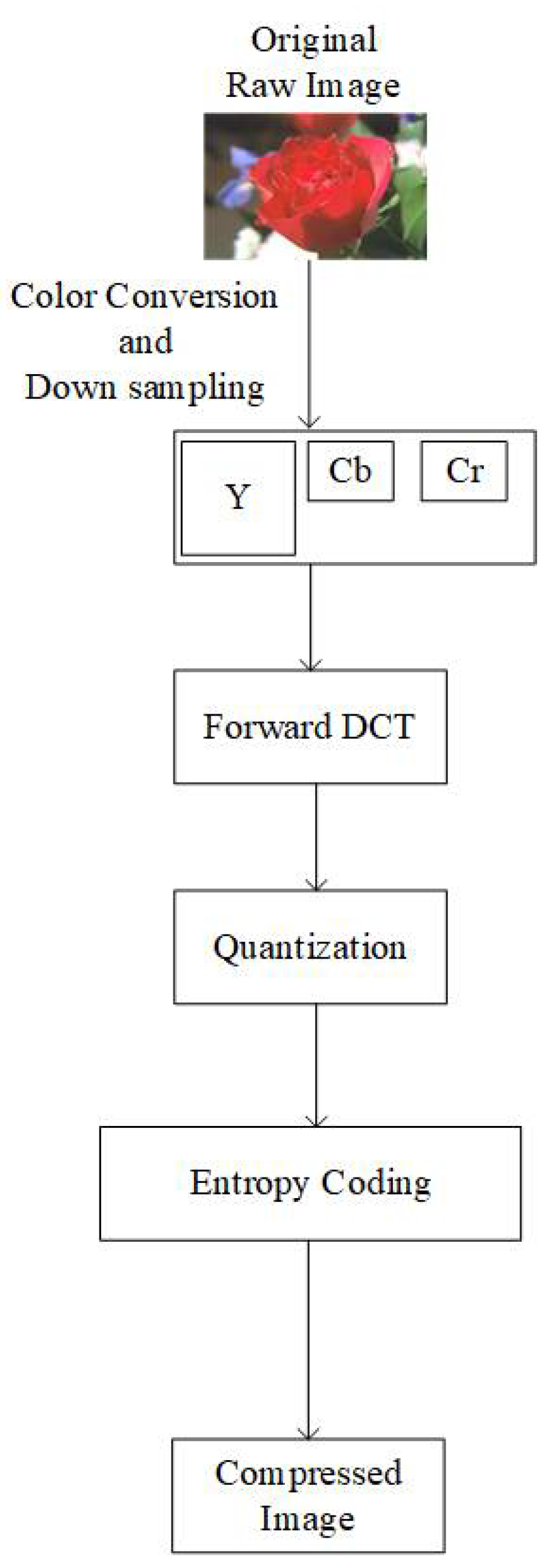
Figure 1 shows the basic overview of the conventional JPEG encoder. YCbCr color components are obtained from the raw input image in the first step. Based on user choice, chroma components Cb and Cr are downsampled to the 4:2:2 or 4:2:0 type [
4]. Each channel is divided into 8 × 8 blocks. A discrete cosine transform (DCT) is applied on the 8 × 8 blocks in the order from left-to-right and top-to-bottom.
After the DCT, blocks are forwarded for quantization. Luma and Chroma components are quantized using different quantization tables [
3]. Quantization tables are generated based on quality factors (QF). The compression ratio and quality of the image are controlled by the QF value. To reduce the redundancy of consecutively occurring DC coefficients, the differential pulse code modulation (DPCM) method is used. In the end, all the processed data is forwarded to the entropy coding module.
2.2. Entropy Coding
Data obtained after quantization need to be stored without losing any information. However, instead of saving the data as-is, JPEG compression performs an additional step of entropy coding. Entropy coding achieves additional compression by encoding the quantized DCT coefficients more efficiently based on their statistical characteristics [
1]. An individual JPEG compression process uses one of two available entropy coding algorithms, either Huffman [
5] or arithmetic encoding [
6].
2.2.1. Huffman
Huffman coding is an entropy encoding algorithm using a variable-length code table. This table has been derived based on the estimated probability of occurrence for each possible value of the source symbol (such as a character in a file) [
1]. The principle of Huffman coding is to assign lower bits to the more frequently occurring data [
7]. A dictionary associating each data symbol with a codeword has the property that no codeword in the dictionary is a prefix of any other codeword in the dictionary [
8].
In the JPEG encoder, Huffman coding is combined with run-length coding (RLC) and is called the run-amplitude Huffman code [
9]. This code represents the run-length of zeros before a nonzero coefficient and the size of that coefficient. The code is then followed by additional bits precisely defining the coefficient amplitude and sign [
4,
9]. The end-of-block (EOB) marker is coded when the last nonzero coefficient occurs. This strategy is omitted in the rare case that the last element of the 8×8 block is nonzero. In the case of an empty block, i.e., where all AC coefficients are zero, the encoder codes an EOB.
2.2.2. Arithmetic
Compared to Huffman coding, arithmetic coding bypasses the mechanism of assigning a specific code to an input symbol. An interval (0, 1) is divided into several sub-intervals based on the occurrence probability of the corresponding symbol. The ordering sequence is known to both the encoder and decoder. In arithmetic coding, unlike Huffman coding, the number of bits assigned to encode each symbol varies according to their assigned probability [
10]. Symbols with lower probability are assigned higher-bit encodings compared to symbols with higher probability, and their probability decreases in inverse proportion to the probability of the occurrence of the character [
1]. The key idea of arithmetic encoding is to assign each symbol an interval. Further, each symbol is divided into subintervals equal to their probability [
11].
Both Huffman and arithmetic encoding are performed on the data without filtering out empty AC coefficient blocks, which decreases the compression ratio.
3. Proposed Algorithm
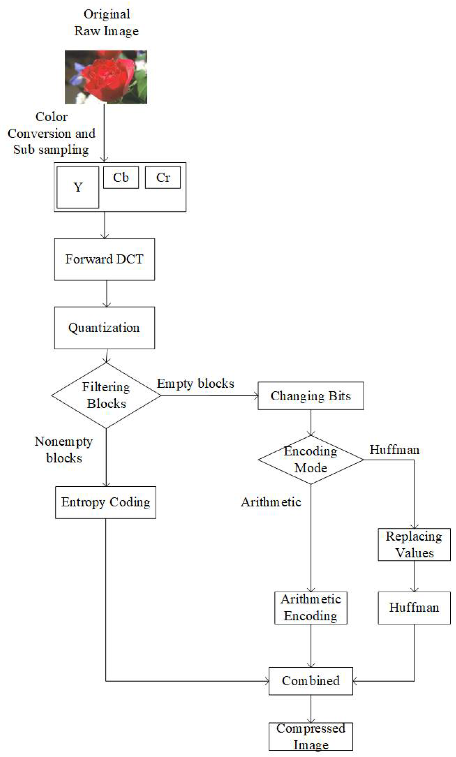
Our proposed algorithm is based on the filtration of 8 × 8 blocks.
Figure 2 shows an overview of the proposed JPEG image coding. To maintain equivalent complexity between the conventional and our proposed entropy coding, we used separate modes for arithmetic and Huffman coding. Before forwarding the 8 × 8 blocks to the JPEG entropy encoder, we perform three steps. These three steps are named as (1) filtration of blocks, (2) changing bits, and (3) replacing values. The third step (
Section 3.3) is performed only in the case of the Huffman encoding mode. It should be noted that the whole process explained in this section is lossless. During the decoding process, we perform the inverse of these steps, and at the end of the inverse process, we know about the location of empty blocks. Moreover, this process has no additional consequences, as we do not change any of the coefficient values.
3.1. Filtration of Blocks
In our proposed algorithm, instead of allowing the encoder to encode the EOB marker for the empty blocks along with the array of non-empty blocks, all the empty blocks are filtered out, and information on the location of empty and non-empty blocks is stored in a separate binary buffer. In this buffer, we store 0 for empty blocks and 1 for non-empty blocks. In the JPEG encoder, the Y component is compressed using a different quantization table compared to the Cb and Cr components. Due to the different nature of their compression, we use separate buffers for the Y, Cb, and Cr components at this stage. Finally, all buffers for Y, Cb, and Cr are concatenated.
3.2. Changing Bits
After concatenating Y, Cb, and Cr buffers, we improve the consistency of identical bit sequence occurrences by replacing all the bit values with 0, except the initial bit 1, only in the case where the next bit is different from the current. In this process, identical occurrences of either 0- or 1-bit values are saved as 0. Thus, we further increase the occurrence of zero bits. For example, suppose we have a sequence of bits as “000011110111”. We have four consecutive zeros followed by four consecutive ones, indicating that a change occurs at the 5th bit in the sequence. Then, we can observe that the next change occurs at the 9th and 10th bit in the sequence. Hence, the sequence is transformed to “000010001100” with bit 1 placed where the change in the sequence occurs.
In the case of arithmetic encoding mode, after performing this step, we provide our buffer to the binary arithmetic encoder [
12]. The remaining of the 8 × 8 blocks, where a nonzero AC coefficient existed, were encoded in a conventional way. After the compression process was completed, we appended our compressed buffer to the remainder of the encoded file.
3.3. Replacing Values
This step is performed only when the selected encoding mode is Huffman. By observing the nature of Huffman encoding, we can save more space if we convert our data, resulting from
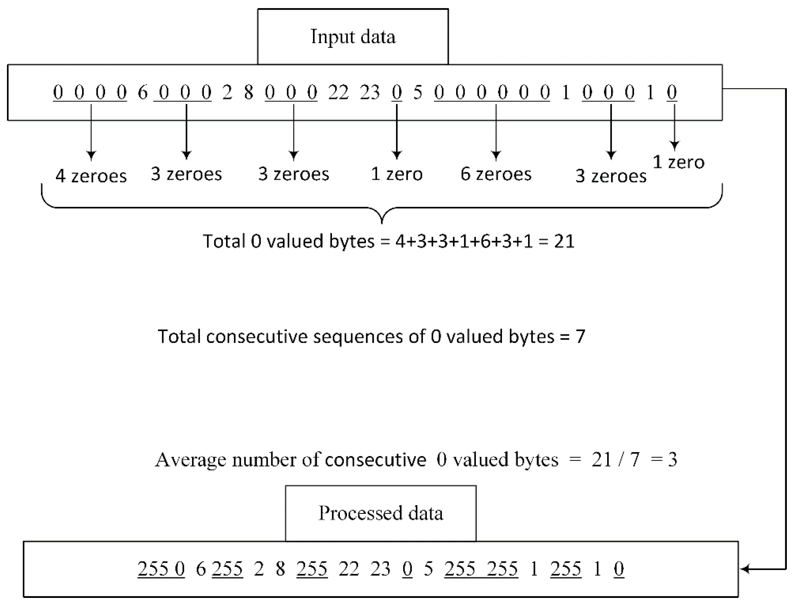
Section 3.2, from bits to bytes. Thus, before replacing the values, bits are converted into bytes. After the conversion, there are still long sequences of consecutive zero-valued bytes present, and to get rid of those long sequences, we perform the step of replacing values. Firstly, we calculate the average number of consecutive zero-valued bytes. The average is used because different types of images have different data. For example, in the case of homogeneous images, the average number of consecutive zeros should be higher owing to a larger amount of empty 8 × 8 blocks present consecutively, whereas, in the case of more detailed images, a smaller number of consecutive empty 8 × 8 blocks are present. The number of consecutively occurring zero-valued bytes equal to the calculated average number is replaced with a less frequently occurring byte value, i.e., 255. In the example shown in
Figure 3, there are two data buffers; input data is the data obtained after converting the values from bits to bytes, while the other one is the processed data.
The total number of zeros was equal to 21 in the original data buffer. These 21 zeros occurred in seven sequences of consecutive zeros. To obtain the average number of consecutively occurring zeros, we divided the total number of zeros with the number of consecutively occurring sequences. Thus, we obtained an average number of zero-valued bytes of three and replaced all three consecutively occurring sequences of three zeros with a constant value of 255.
In the case of floating-point results after division, we round it to the nearest integer. If a byte value of 255 occurs in the input data, we tail it with an additional byte value, e.g., 217, in order to differentiate between a replaced value of 255 and an input data value of 255. The example in
Figure 3 demonstrates that after replacement, a sequence with a data size of 29 bytes was reduced to 19 bytes.
As the third step is performed only in the case of JPEG Huffman mode, the processed data is designated for Huffman encoding. After the compression process was completed, we appended our compressed buffer to the remainder of the encoded file.
4. Experimental Results
We conducted an experiment on 15 test images using libjpeg-turbo [
13] version 2.0.5. All test images were taken from the JPEG AI dataset [
14]. These 15 images, shown in
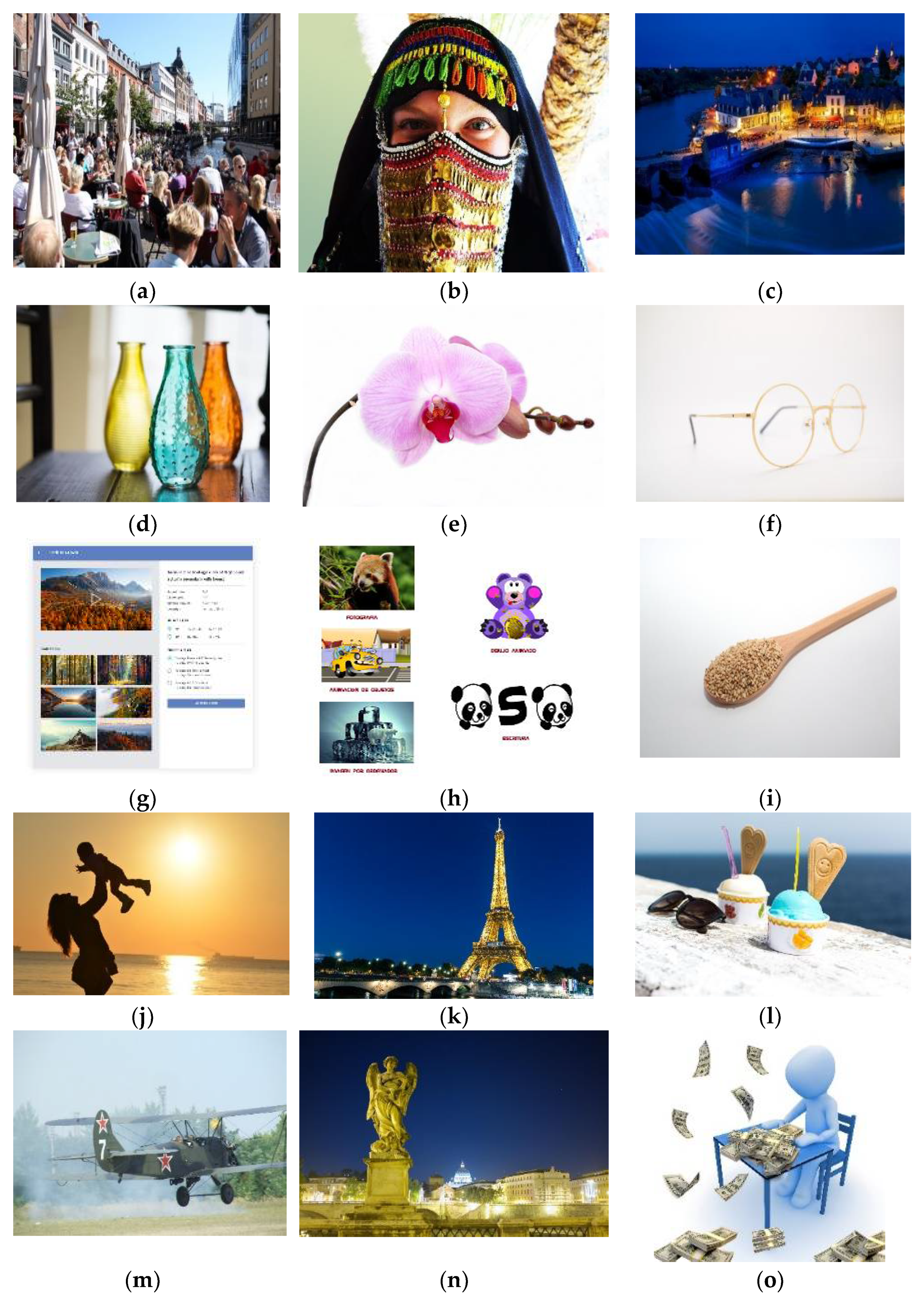
Figure 4, were selected carefully. They include two screenshots, two homogenous images, one image of night view, one image of street daytime view, one item close-up, one human close-up image, and seven additional random images. Thus, in these 15 test images, we included a broad variety of major types of images to obtain a useful and indicative result.
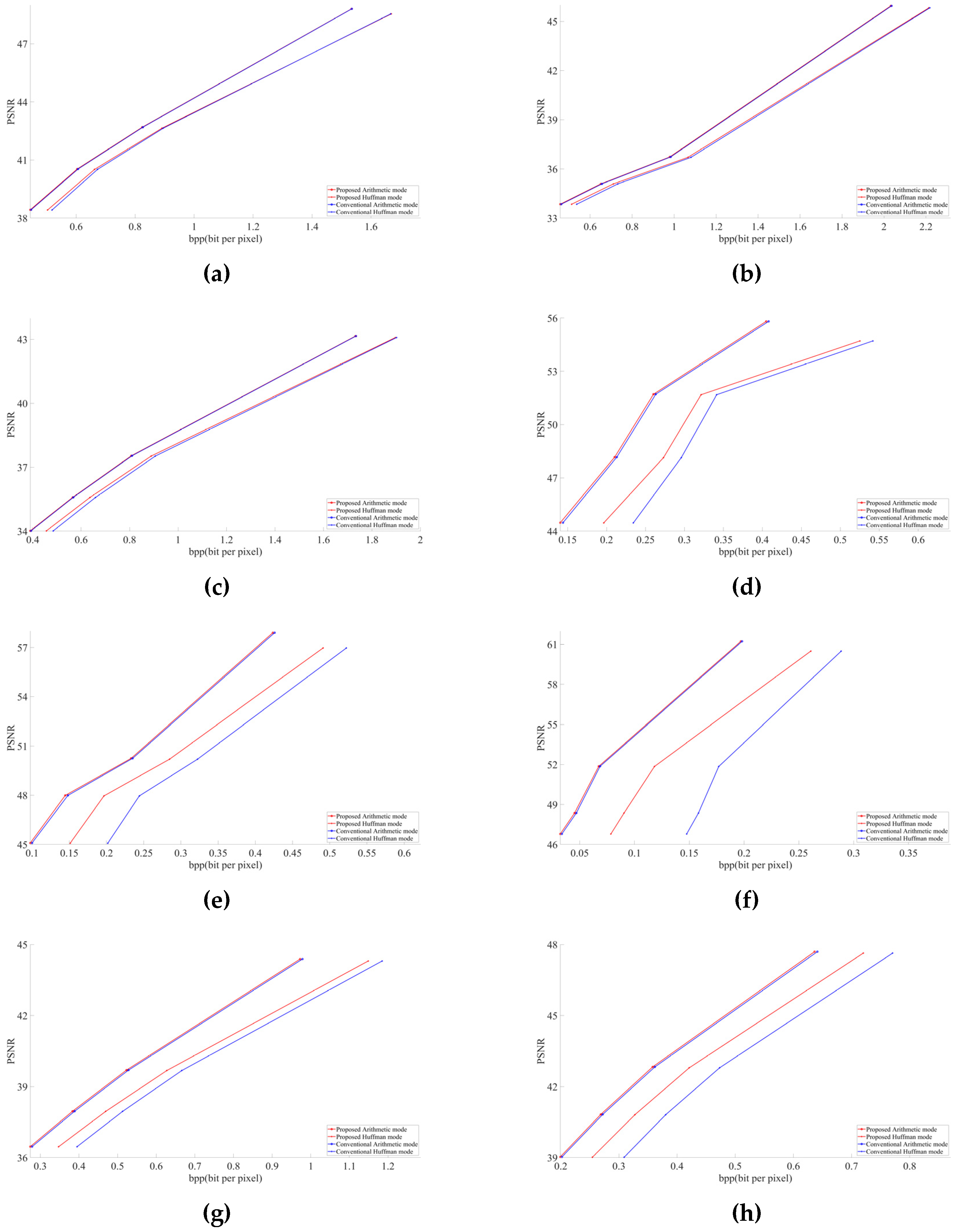
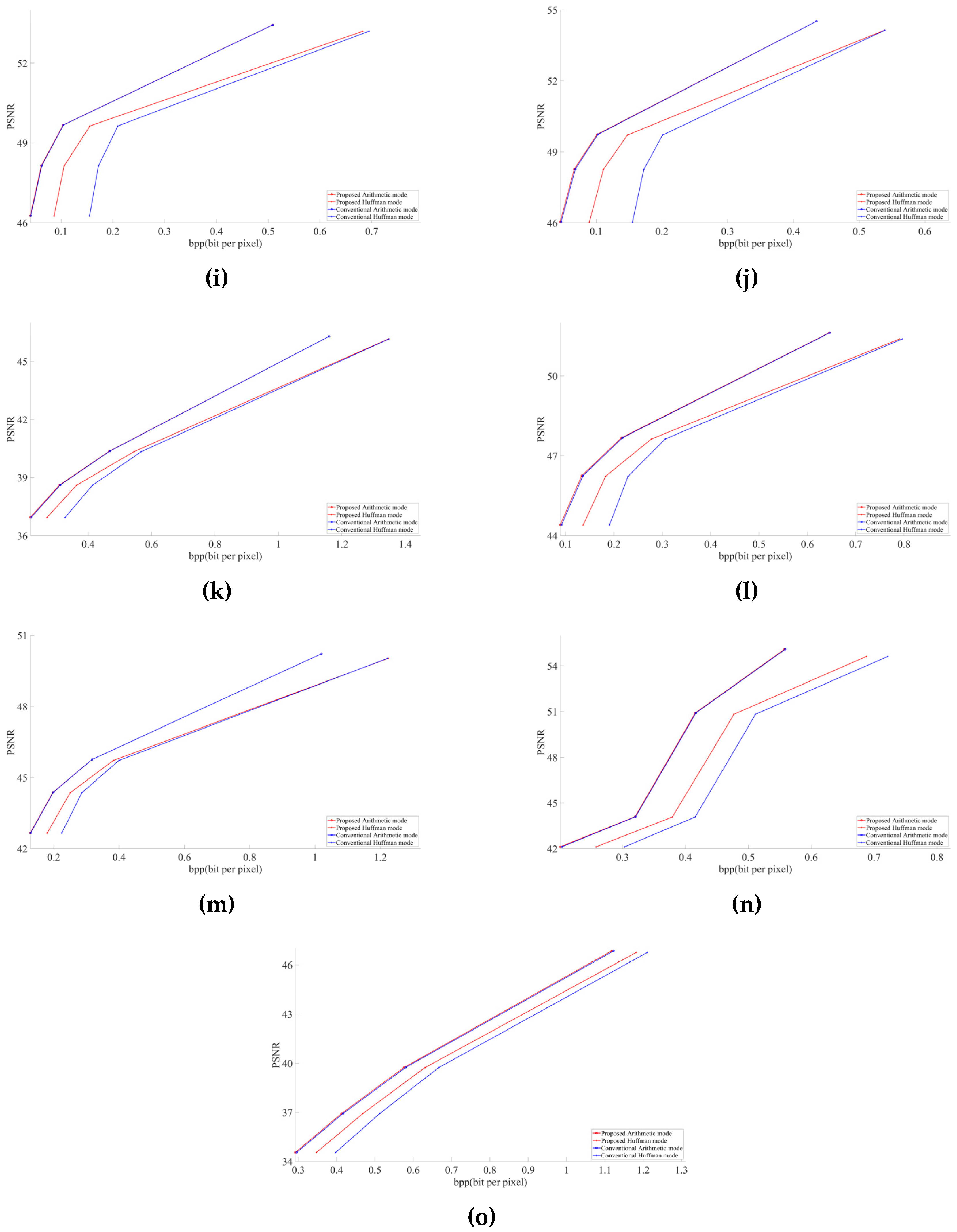
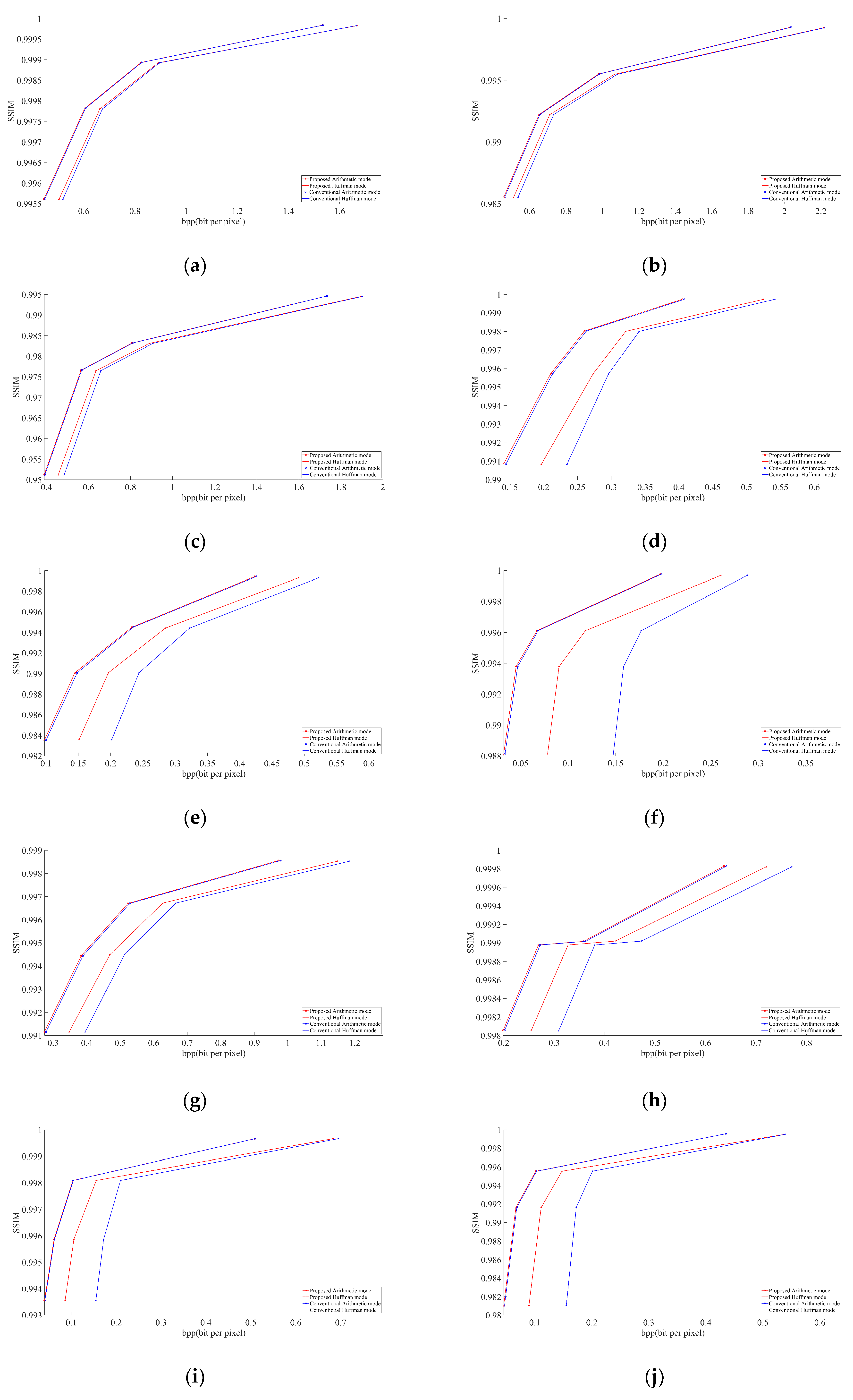
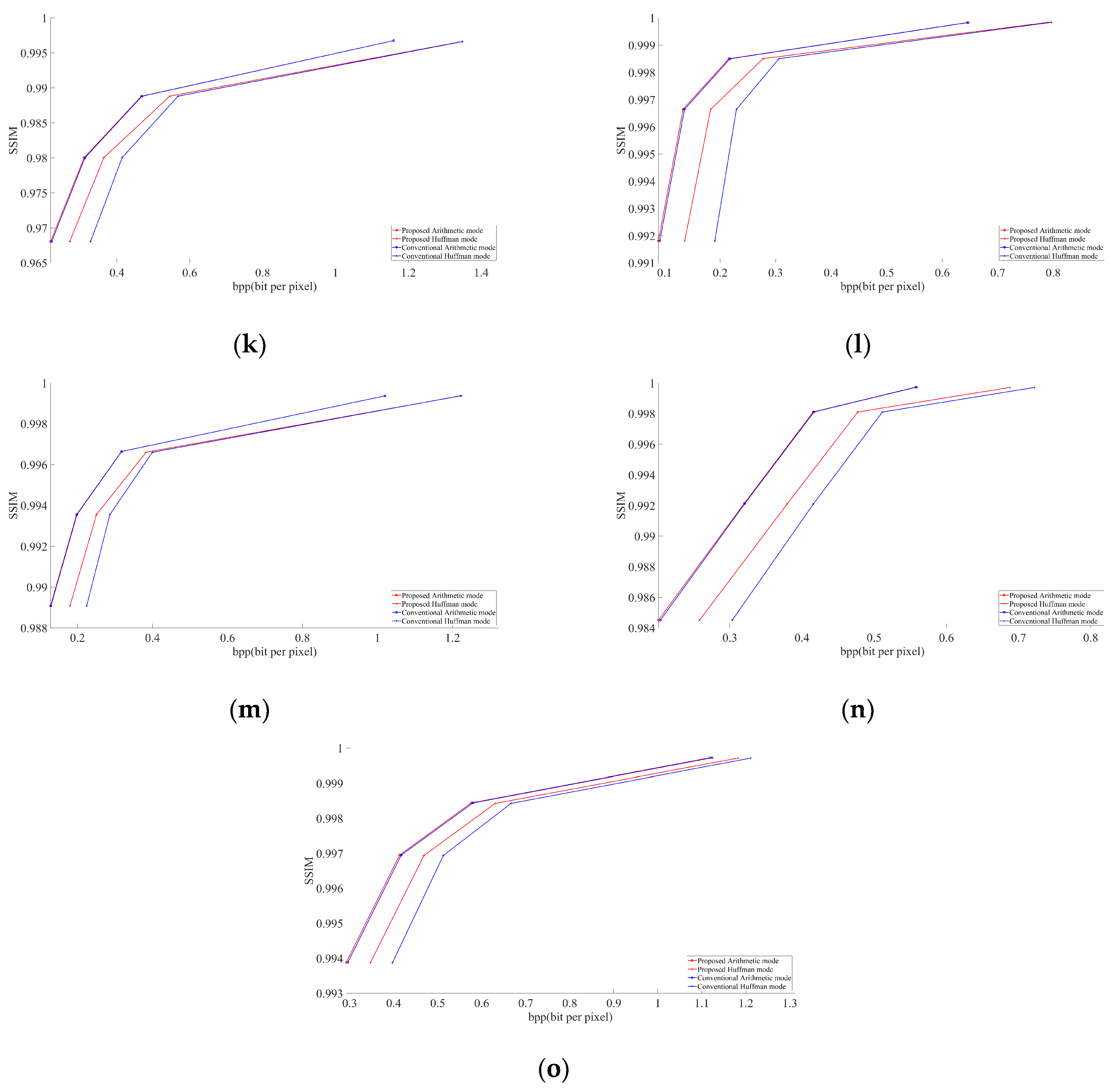
Figure 5 and
Figure 6 describe the graphical results for all the test images shown in
Figure 4. The
Y-axis represents the PSNR and SSIM values respectively in
Figure 5 and
Figure 6, whereas the
X-axis represents the BPP.
As discussed in
Section 2.1, chroma components Cb and Cr are downsampled to the 4:2:2 or 4:2:0 type in JPEG [
4]. In this paper, we targeted the 4:2:0 subsampling at different QF ranging from low to high to obtain a better and clearer result. The selected QF values were 30, 50, 70, and 90. Graphs were obtained using MATLAB R2020a. We considered PSNR (peak signal-to-noise) and BPP (bits per pixel) to evaluate our obtained results. Compressed buffers after the step detailed in
Section 3.2 for arithmetic and after the step is given in
Section 3.3 for Huffman were included in the file size for calculating BPP. All the images decoded with the modified JPEG decoder had the same PSNR as the images decoded by the conventional JPEG decoder. This shows the successful implementation of our modified decoder.
In all images, our proposed approach achieved significant improvements. The demonstrated improvement in the case of homogeneous images was greater than for complex images. Among the test images used in the experiment,
Figure 4f showed the best result. The proposed algorithm is tested only for high-resolution and original images. The lowest image resolution was 1980 × 1272 among the test images shown in
Figure 5. Due to the high possibility of consecutive empty DCT 8 × 8 blocks, the proposed algorithm is considered useful in high-resolution images. To calculate the average gain in BPP for both Huffman and arithmetic mode, shown in
Table 1, we used Bjontegaard’s metric [
15,
16,
17].
In
Table 2 and
Table 3, for Huffman and Arithmetic encoding mode, respectively, we describe the test images actual file size encoded by the conventional JPEG encoder [
13], file size when we filtered out the empty blocks, and the difference between actual file size and when we excluded the empty blocks from encoding. This difference indicates the size taken by the empty blocks in encoded images. We added another column of the proposed method. It shows the additional data required by the proposed method to encode the empty blocks and their locations. Moreover, the column named “Gain” in
Table 2 and
Table 3 represents the ratio of the size required to encode the empty blocks by the conventional JPEG encoder to the proposed JPEG encoder. All the sizes in
Table 2 and
Table 3 are calculated in bytes.
5. Conclusions
In this paper, we have proposed an improved version of the conventional JPEG algorithm. Based on experimental results, we concluded that the proposed algorithm increases the compression ratio. In other words, a higher quality image can be obtained at the same BPP.
A good balance between quality and BPP is always a major concern in the field of image processing. In the market, almost all social networks use JPEG encoders and compress images prior to sending. Compression is required due to storage resource restrictions on local and remote servers. If all users were to send and store images at their original quality, then storage space resource requirements would become an even more significant issue.
The conventional JPEG encoder uses both Huffman and arithmetic entropy encoding modes. Thus, to maintain an equivalent complexity level between the conventional and our proposed entropy coding, if the arithmetic encoding mode is selected in conventional JPEG, we used an arithmetic encoder to compress the additional data; otherwise, the Huffman encoder was used. Other than Huffman encoding and arithmetic encoding, the remaining steps are very simple. Thus, the complexity difference is negligible.
Our experimental results demonstrate that at the same PSNR value as the conventional JPEG encoder, the modified JPEG encoder shows better performance in terms of BPP, as shown in
Figure 5 and
Table 1. In the future, we may implement the same scenario in other image encoding methods.
Author Contributions
Conceptualization, Y.I. and O.-J.K.; methodology, Y.I.; software, Y.I.; validation, Y.I. and O.-J.K.; formal analysis, O.-J.K.; investigation, O.-J.K.; resources, Y.I.; data curation, Y.I.; writing—original draft preparation, Y.I.; writing—review and editing, O.-J.K.; visualization, Y.I; supervision, O.-J.K.; project administration, O.-J.K.; funding acquisition, O.-J.K. Both authors have read and agreed to the published version of the manuscript.
Funding
This research was funded by the Institute of Information & communications Technology Planning & Evaluation (IITP), grant number No.2020-0-00347.
Institutional Review Board Statement
Not applicable.
Informed Consent Statement
Not applicable.
Data Availability Statement
Restrictions apply to the availability of these data. All test images were obtained from JPEG-AI dataset. They are available at “JPEG AI image coding common test conditions”, ISO/IEC JTC1/SC29/WG1 N84035, 84th Meeting, Brussels, Belgium (July 2019).
Acknowledgments
This work was supported by the Institute for Information & communications Technology Promotion (IITP) grant funded by the Korea government (MSIT) (No.2020-0-00347, Development of JPEG Systems standard for snack culture contents).
Conflicts of Interest
The authors declare no conflict of interest.
References
- Yang, M.; Bourbakis, N. An overview of lossless digital image compression techniques. In Proceedings of the 48th Midwest Symposium on Circuits and Systems, Covington, KY, USA, 7–10 August 2005; Volume 2, pp. 1099–1102. [Google Scholar] [CrossRef]
- Cai, Q.; Song, L.; Li, G.; Ling, N. Lossy and lossless intra coding performance evaluation: HEVC, H.264/AVC, JPEG 2000 and JPEG LS. In Proceedings of the 2012 Asia Pacific Signal and Information Processing Association Annual Summit and Conference, Hollywood, CA, USA, 3–6 December 2012; pp. 1–9. [Google Scholar]
- Pennebaker, W.B.; Mitchell, J.L. JPEG: Still Image Data Compression Standard; Springer Science & Business Media: Berlin, Germany, 1992. [Google Scholar]
- Wallace, G.K. The JPEG still picture compression standard. IEEE Trans. Consum. Electron. 1992, 38, xviii–xxxiv. [Google Scholar] [CrossRef]
- Huffman, D.A. A method for the construction of minimum-redundancy codes. Proc. IRE 1952, 40, 1098–1101. [Google Scholar] [CrossRef]
- Pennebaker, W.B.; Mitchell, J.L. Arithmetic coding articles. IBM J. Res. Dev. 1988, 32, 717–774. [Google Scholar] [CrossRef]
- Sharma, M. Compression using huffman coding. Int. J. Comput. Sci. Netw. Secur. 2010, 10, 133–141. [Google Scholar]
- Mitzenmacher, M. On the hardness of finding optimal multiple preset dictionaries. IEEE Trans. Inf. Theory 2004, 50, 1536–1539. [Google Scholar] [CrossRef] [Green Version]
- Kingsbury, N. 4F8 Image Coding Course. Lect. Notes. 2016. Available online: http://sigproc.eng.cam.ac.uk/foswiki/pub/Main/NGK/4F8CODING.pdf (accessed on 15 July 2021).
- Shahbahrami, A.; Bahrampour, R.; Rostami, M.S.; Mobarhan, M.A. Evaluation of Huffman and arithmetic algorithms for multimedia compression standards. arXiv 2011, arXiv:1109.0216. [Google Scholar] [CrossRef]
- Kavitha, V.; Easwarakumar, K.S. Enhancing privacy in arithmetic coding. ICGST-AIML J. 2008, 8, 1. [Google Scholar]
- Mahoney, M. Data Compression Explained. Available online: mattmahoney.net (accessed on 15 July 2021).
- Independent JPEG Group. Available online: https://libjpeg-turbo.org (accessed on 15 July 2021).
- Ascenso, J.; Akayzi, P. JPEG AI image coding common test conditions. In Proceedings of the ISO/IEC JTC1/SC29/WG1 N84035, 84th Meeting, Brussels, Belgium, 13–19 July 2019. [Google Scholar]
- Bjontegaard, G. Calculation of average PSNR differences between RD-curves. VCEG-M33 2001. [Google Scholar]
- Pateux, S.; Joel, J. An excel add-in for computing Bjontegaard metric and its evolution. ITU-T SG16 Q 6 2007, 7. [Google Scholar]
- VCEG-M34. Available online: http://wftp3.itu.int/av-arch/video-site/0104_Aus/VCEG-M34.xls (accessed on 15 July 2021).
| Publisher’s Note: MDPI stays neutral with regard to jurisdictional claims in published maps and institutional affiliations. |
© 2021 by the authors. Licensee MDPI, Basel, Switzerland. This article is an open access article distributed under the terms and conditions of the Creative Commons Attribution (CC BY) license (https://creativecommons.org/licenses/by/4.0/).


