Abstract
The goal of no-reference image quality assessment (NR-IQA) is to predict the quality of an image as perceived by human observers without using any pristine, reference images. In this study, an NR-IQA algorithm is proposed which is driven by a novel feature vector containing statistical and perceptual features. Different from other methods, normalized local fractal dimension distribution and normalized first digit distributions in the wavelet and spatial domains are incorporated into the statistical features. Moreover, powerful perceptual features, such as colorfulness, dark channel feature, entropy, and mean of phase congruency image, are also incorporated to the proposed model. Experimental results on five large publicly available databases (KADID-10k, ESPL-LIVE HDR, CSIQ, TID2013, and TID2008) show that the proposed method is able to outperform other state-of-the-art methods.
1. Introduction
Visual signals (digital images or videos) undergo a wide variety of distortions during acquisition, compression, transmission, and storage. Thus, image quality assessment (IQA) is crucial to predict the quality of digital images in many applications, such as compression, communication, printing, display, analysis, registration, restoration, and enhancement [1,2,3,4]. Generally, it can be used in benchmarking any image processing algorithms. Furthermore, it is indispensable in evaluating any new hardware or software component related to imaging. For instance, a number of biometric algorithms rely on images, such as palmprint, fingerprint, face image, or handwriting recognition. However, the acquisition process of images is often not perfect in practice. Because of this, information about the quality degradation of images is required [5]. Similarly, the performance of object detection (e.g., pedestrian, car, traffic sign, etc.) algorithms heavily depends on the image quality [6,7]. As a consequence, monitoring image/video quality is also crucial in vision-based advanced driver-assistance systems [8].
Since human observers are the end users of visual content, the quality of visual signals is ideally evaluated by subjective user studies in a laboratory environment involving specialists. During these user studies, subjective quality scores are collected from each participant. Subsequently, the quality of a visual signal is given by mean opinion score (MOS), which is defined as the arithmetic mean of the individual ratings. In most cases, an absolute category rating (ACR) scale is applied where the range usually goes from 1.0 (very poor quality) to 5.0 (excellent quality). Several international standards such as ITU BT.500-13 [9] or ITU P910 [10] have been proposed for performing subjective visual quality assessment. As already mentioned, the main goal of subjective visual quality assessment is to assign a score of the users’ perceived quality to each visual signal in a given set of signals (images or videos). However, the resulted assessment might vary significantly because of many factors such as lighting conditions and the choice of the subjects. That is why ITU-R BT.500-13 [9] gives detailed recommendations about viewing conditions, monitor resolution, selection of test materials, observers, test session, grading scales, analysis and interpretation of the results.
Subjective visual quality assessment has some drawbacks which limit their applications. Namely, they are time-consuming and expensive because subjective results are obtained through experiments with many observers. As a consequence, they cannot be part of real-time applications such as image transmission systems. Therefore, the development of objective visual quality assessment methods that are able to predict the perceptual quality of visual signals is of high importance. The classification of objective visual quality assessment algorithms is based on the availability of the original (reference) signal. If a reference signal is not available, a visual quality assessment algorithm is regarded as a no-reference (NR) one. NR algorithms can be classified into two further groups, where the so-called distortion-specific NR algorithms assume that a specific distortion is present in the visual signal, whereas general purpose (or non-distortion specific) algorithms operate on various distortion types. Reduced-reference (RR) methods retain only part of the information from the reference signal, whereas full-reference (FR) algorithms have full access to the complete reference medium to predict the quality scores. Similar to NR methods, FR algorithms can be also classified into distortion-specific and general purpose ones. The research of objective visual quality assessment demands databases that contain images or videos with the corresponding MOS values. To this end, a number of image or video quality databases have been made publicly available. According to the database structure, these databases can be categorized into three groups. The first one contains a smaller set of pristine, reference visual signals and artificially distorted images derived from the pristine visual signals considering different artificial distortions at different intensity levels. The second group contains only digital images or videos with authentic distortions collected from photographers, so pristine images or videos cannot be found in such databases. As a consequence, the development of FR methods is connected to the first group of databases. In contrast, NR-IQA algorithms can be trained and tested on both types of databases.
The rest of this section is organized as follows. In Section 1.1, the related and previous work in NR-IQA are reviewed. The main contributions of this study are declared in Section 1.2. The structure of this paper is described in Section 1.3.
1.1. Related Work
Previous and related work are introduced in this section, including a brief review of distortion-specific, opinion aware, and opinion unaware methods. The so-called distortion-specific methods presume one or several types of distortions in the image, such as blur [11], blockiness [12], ringing [13], or JPEG2000 noise [14]. The disadvantage of this line of work is quite obvious. Namely, the number of possible image distortion and noise types is large, while they are able to consider only several noise types. In contrast, general opinion aware methods are trained on features extracted from distorted images to predict perceptual quality over various types of image distortions. For example, the blind image quality indices (BIQI) [15] method contains two stages. First, the distortion present in the image is determined with the help of a trained support vector machine (SVM) [16] given a set of image noise types. Second, the perceptual quality is evaluated with respect to the distortion. Numerous opinion aware methods are based on the so-called natural scene statistics (NSS) which is a subfield of perception and deals with the statistical regularities of natural scenes. More specifically, it is assumed that natural images have certain statistical regularities which are biased by visual distortions. That is why, NSS have become successful in perceptual image and video quality prediction. For instance, Saad et al. [17] devised a statistical model in the discrete cosine transform (DCT) domain. Specifically, it utilizes a Bayesian approach to predict perceptual quality based on a set of DCT coefficients related features. In contrast, Lu et al. [18] assumed that image distortions can be characterized in the wavelet domain. On the other hand, Lu et al. [19] developed an NSS model in the contourlet domain. Namely, the statistics of contourlet coefficients was used to estimate image quality. In blind/referenceless image spatial quality evaluator [20] (BRISQUE), scene statistics of locally normalized luminance coefficients are applied to train a support vector regressor [21] (SVR) for perceptual quality prediction. In the spatial domain, image gradient magnitude have been used by many researchers to predict image quality [22,23,24]. Specifically, Xue et al. [23] utilizes the joint local contrast features from the gradient magnitude map and the Laplacian of Gaussian response. In feature maps based referenceless image quality evaluation engine (FRIQUEE) [25], a large set of features is defined using perceptually relevant color and transform domain spaces. Liu et al. [26] extracted features from the distorted images’ curvelet domain and trained an SVM for perceptual quality prediction. In contrast, Li et al. [27] extracted features from the distorted images with the help of shearlet transform. Subsequently, stacked autoencoders were applied to make these features more discriminative. Finally, a softmax classifier was used for quality prediction. Ou et al. [28] were the first who applied Benford’s law in image quality assessment. Namely, they pointed out features based on Benford’s law are very sensitive to white noise, Gaussian blur, and fast fading. Freitas et al. [29] combined the statistics of different color and texture descriptors and mapped onto quality scores using a gradient boosting machine. In an other study, Freitas et al. [30] compared the performance of different local binary pattern texture descriptors for NR-IQA.
Opinion unaware methods require neither training images of distortions nor perceptual quality scores. For example, Mittal et al. [31] extracted BRISQUE [20] features from image patches and perceptual quality was defined as the distance between the NSS-based features extracted from the test image to the features obtained from the target IQA database. Moreover, these features were approximated by multivariate Gaussian distributions. This method was further developed by Zhang et al. [32] who incorporated more quality aware features and a local quality measurement procedure into the previous model. In contrast, Xue et al. [33] proposed a quality-aware clustering strategy to determine a set of cluster centroids. Next, these centroids were utilized as a codebook to estimate perceptual image quality.
1.2. Contributions
The main contributions of this study are as follows. An NR-IQA method is introduced which is driven by a novel feature vector. Furthermore, it contains new elements which cannot be found in previous methods. Namely, this is the first work that applies local fractal dimension distribution of an image for NR-IQA. Although Ou et al. [28] derived first quality aware features with the help of Benford’s law, the proposed method directly measures the first digit distribution in the wavelet and spatial domain to define features. Moreover, the above mentioned novel statistical features are enriched with powerful perceptual features, such as colorfulness, global contrast factor, dark channel feature, entropy, and mean of phase congruency image. Experimental results on five large publicly available quality databases show that the proposed method is able to significantly outperform other state-of-the-art methods. This paper is accompanied by the source code of the proposed method (https://github.com/Skythianos/SPF-IQA).
1.3. Structure
2. Methodology
The general overview of the proposed method is depicted in Figure 1. Statistics and perceptual features are extracted from the input image which are mapped onto perceptual quality scores with the help of a regression technique. Specifically, the statistics features are used to capture the differences between the statistical patterns of pristine, natural images and those of distorted images. To this end, the fractal dimension distribution, the first digit distribution in the wavelet and gradient magnitude domain, and color statistics features are extracted. Since some perceptual features consistent with human quality judgements, the following perceptual features are incorporated into the proposed model: colorfulness, global contrast factor, dark channel feature, entropy, and mean of phase congruency image.
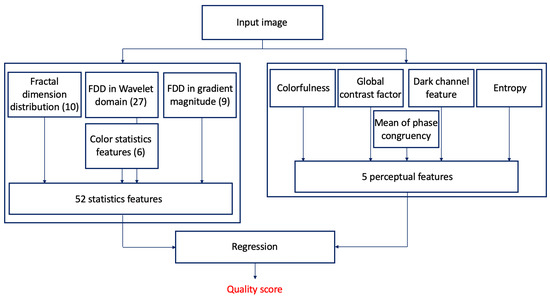
Figure 1.
Architecture of the proposed no-reference image quality assessment method.
The rest of this section is organized as follows. The proposed statistical features are introduced in Section 2.1, while the used perceptual features are described in Section 2.2.
2.1. Statistical Features
- Local fractal dimension distribution: Fractal analysis was first proposed by Mandelbrot [34] and it deals with the study of irregular and self-similar objects. By definition, fractal dimenstion characterizes patterns or sets “by quantifying their complexity as a ratio of the change in detail to the change in scale” [34]. The fractal dimension image is produced by considering each pixel in the original image as a center of a 7-by-7 rectangular neighborhood and the fractal dimension is calculated from this neighborhood. To determine the fractal dimension of a grayscale image patch, the box counting technique developed by Al-Kadi and Watson [35] was applied. From the fractal dimension image, a 10-bin normalized histogram was calculated considering the values between −2 and 3. Figure 2 illustrates the local fractal dimension images of a reference and a distorted image. It can be observed that the fractal dimension of an image patch is extremely sensitive to image distortions.
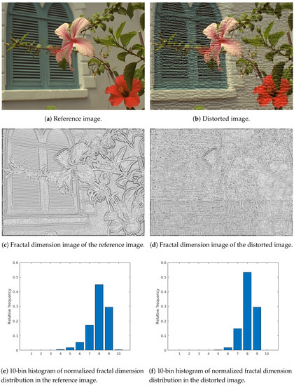 Figure 2. Illustration to fractal dimension distribution. Fractal dimension images are produced by considering each pixel in the original image as a center of a 7 × 7 patch and the fractal dimension is calculated from this patch. Furthermore, black pixels correspond to −2 fractal dimension, while white ones correspond to +3.
 - First digit distribution in wavelet domain: Benford’s law, also called the first digit law, states leading digit in many real-world datasets occurs with probabilityMore specifically, Benford’s law [36] works on a distribution of numbers if that distribution spans quite a few order of magnitudes. As pointed out in [37], the first digit distribution in the transform domain of a pristine natural image harmonizes better with the Benford’s law than those of a distorted image. In this study, the normalized first digit distribution is utilized in the wavelet domain and in the image gradient domain to extract feature vectors. Specifically, an Fejér-Korovkin wavelet [38] was used to transform the image into wavelet domain. Next, the normalized first digit distribution was measured in horizontal detail coefficients, vertical detail coefficients, and diagonal detail coefficients. Finally, a 27-dimensional feature vector was obtained in the wavelet domain by concatenating the normalized first digit distributions in the horizontal, vertical, and diagonal detail coefficients, respectively.
- First digit distribution in gradient magnitude: The gradient of the image was determined with the help of 3-by-3 Sobel operator. The normalized first digit distribution of the gradient magnitude image was measured and a 9-dimensional feature vector was compiled.Table 1 illustrates the average and median Euclidean distances between first digit distributions of TID2013 [39] images in the wavelet and gradient magnitude domain and Benford’s law prediction. It can be observed that the first digit distributions in the wavelet domain is almost the same as Benford’s law prediction. Moreover, it can be clearly seen that the distorted images distance from Benford’s law is significantly larger than those of the reference images. One can further observe that the most distorted images’ first digit distribution Euclidean distance from the Benford’s law is the largest, since the standard deviation of the distance values for the distorted images is three times larger than those of the reference images. In the gradient magnitude domain, the above mentioned observations are less significant. Furthermore, the standard deviations are almost the same.
 Table 1. Mean and median distances from the Benford’s law in TID2013 [39] measured in the wavelet (horizontal, vertical, and diagonal detail coefficients) and spatial (gradient magnitude) domains.
 - Color statistics features: To extract the statistical properties of the color, the model of Ruderman et al. [40] was applied. Specifically, an RGB image was first transformed into a mean-subtracted logarithmic signal:where , , and are the mean values of the logarithms of the R, G, and B image channels, respectively. From these signals, the following , , and signals are derived:As pointed out by Ruderman et al. [40], the distributions of the coefficients in , , and approximately fit to Gaussian distributions for natural images (see Figure 3 for an example). As a consequence, a Gaussian distribution was fit to the coefficients of , , and . Moreover, the mean and the variance were taken as quality-aware features. As a result, the color statistics feature vector contains six elements (mean and variance for , , and ). Figure 3 illustrates the distribution of values in a reference image and in its distorted counterpart from TID2013 [39] database.
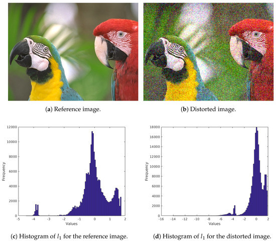 Figure 3. Illustration of l1 values distribution in a reference and a distorted image from TID2013 [39] database.
2.2. Perceptual Features
- Colorfulness: As pointed out in [41], humans prefer slightly more colorful images and colorfulness influence perceptual quality judgements. It was calculated using the following formula [42]:where and stand for the standard deviation and mean of the matrices given in the subscripts. Furthermore, and , where R, G, and B denote the red, green, and blue channels of the input image, respectively.
- Global contrast factor: Humans’ ability to recognize or distinguish objects in the image strongly depends on the contrast. As a consequence, contrast may influence the perceptual quality and is incorporated into the proposed model. In this study, Matkovic et al.’s [43] model was applied which is limited to grayscale contrast. Global contrast factor is computed as follows:where is defined as , . Furthermore, isandwhere L stands for the intensity pixel value of the image after applying gamma correction (). Assuming that the image’s width is w and its height is w, and the image is reshaped into a row-wise one dimensional array.
- Dark channel feature: He et al. [44] called dark pixels those pixels whose intensities in at least one color channel are very low. Specifically, a dark channel was defined as:where denotes the intensity value for a color channel and stands for the image patch centered around pixel x. In this study, the dark channel feature of an image is defined as:where denotes the intensity value for a color channel and stands for an image patch centered around pixel x. Moreover, S denotes the area of the input image.
- Entropy: It has many different interpretations, such as “measure of order” or “measure of randomness”. In other words, it describes how much information is provided by the image. Therefore, it can be applied to characterize the texture of an image. Furthermore, image entropy changes with the type and level of image distortions. Entropy of a grayscale image I is defined as:where is the empirical distribution of the grayscale values.
- Mean of phase congruency image: The main idea behind phase congruency is that perceptually significant image features can be observed at those spatial coordinates where the Fourier series components are maximally in phase [45]. The formal definition of phase congruency (PC) is the following [46],where is the energy of signal x and stands for the nth Fourier amplitude. Equation (15) was developed further by Kovesi [45] by incorporating noise compensation,where weights for frequency spread, and denotes the floor function, T is an estimation for the noise level, and is a small constant for avoiding the division by 0. Furthermore,where is the phase of the nth Fourier component at x and is the average phase at x. Phase congruency was used to detect boundary, texture direction, and image segmentation [47]. In Figure 4, it is illustrated that perceptual quality degradations severely modify the phase congruency image. That is why, the mean of the phase congruency image was used as a perceptual metric in this study.
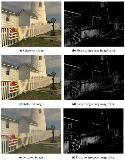 Figure 4. Illustration of phase congruency.
3. Experimental Results
In this section, experimental results and analysis are presented. Specifically, the evaluation protocol is given in Section 3.1. The experimental setup is described in Section 3.2. A parameter study, which reasons the applied design choices, is presented in Section 3.3. Finally, a comparison to other state-of-the-art NR-IQA methods is carried out in Section 3.4.
3.1. Evaluation Protocol
A reliable way to evaluate objective NR-IQA methods is based on measuring the correlation strength between the ground-truth scores of a publicly available IQA database and the predicted scores. In the literature, Pearson’s linear correlation coefficient (PLCC) and Spearman’s rank-order correlation coefficient (SROCC) are widely applied to characterize the degree of correlation. PLCC between vectors x and y can be expressed as
where and . Furthermore, x stands for the vector containing the ground-truth scores, while y vector consists of the predicted scores. SROCC between vectors x and y can be defined as
where the function gives back a vector whose ith element is the rank of the ith element in the input vector. As a consequence, SROCC between vectors x and y can also be expressed as
where and stand for the middle ranks of x and y, respectively. Furthermore, the proposed algorithm and other learning-based state-of-the-art methods were evaluated by 5-fold cross-validation with 20 repetitions. Moreover, average PLCC and SROCC values are reported in this study.
3.2. Experimental Setup
ESPL-LIVE HDR [48], KADID-10k [49], CSIQ [50], TID2013 [39], and TID2008 [51] publicly available IQA databases were used to train and test the proposed algorithm. Table 2 illustrates some facts about the publicly available IQA databases used in this paper. It allows comparisons between the number of reference and test images, image resolutions, the number of distortion levels, and the number of distortion types. KADID-10k [49], CSIQ [50], TID2008 [51], and TID2013 [39] consist of a small set of reference images and artificially distorted images derived from the reference images using different distortion intensity levels and types. In contrast, ESPL-LIVE HDR [48] contains high dynamic range images created by multi-exposure fusion, tone mapping, or post-processing.
Table 2.
Comparison of publicly available IQA databases used in this study.
Specifically, the applied IQA database was divided randomly into a training set (∼80% of images) and a test set (∼20% of images) according to the reference images so no semantic content overlap was between these two sets. Moreover, average PLCC and SROCC values are reported measured over 20 random train-test splits.
3.3. Parameter Study
Once the feature vector is obtained, it must be mapped onto perceptual quality scores. Different machine learning techniques can be used to this end. First, the performance of different regression methods is examined in this section. More specifically, SVR with Gaussian kernel function, SVR with linear kernel function, Gaussian process regression (GPR) with squared exponential kernel function, GPR with rational quadratic kernel function, binary tree regression (BTR), and random forest regression (RFR) are considered in this study. The results for KADID-10k [49], ESPL-LIVE HDR [48], CSIQ [50], TID2013 [39], and TID2008 [51] databases are summarized in Figure 5, Figure 6, Figure 7, Figure 8 and Figure 9. From these results, it can be clearly seen that GPR with rational quadratic kernel function significantly outperforms the other examined regression techniques. As a consequence, GPR with rational quadratic kernel function was used in the further experiments.
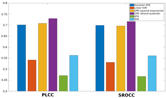
Figure 5.
Comparison of different regression methods (SVR with Gaussian kernel function, SVR with linear kernel function, GPR with squared exponential kernel function, GPR with rational quadratic kernel function, BTR, and RFR). Mean PLCC and SROCC values were measured over 20 random train-test splits on KADID-10k [49].
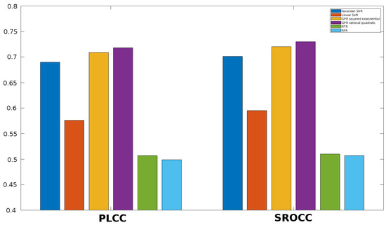
Figure 6.
Comparison of different regression methods (SVR with Gaussian kernel function, SVR with linear kernel function, GPR with squared exponential kernel function, GPR with rational quadratic kernel function, BTR, and RFR). Mean PLCC and SROCC values were measured over 20 random train-test splits on ESPL-LIVE HDR [48].
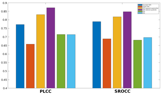
Figure 7.
Comparison of different regression methods (SVR with Gaussian kernel function, SVR with linear kernel function, GPR with squared exponential kernel function, GPR with rational quadratic kernel function, BTR, and RFR). Mean PLCC and SROCC values were measured over 20 random train-test splits on CSIQ [50].
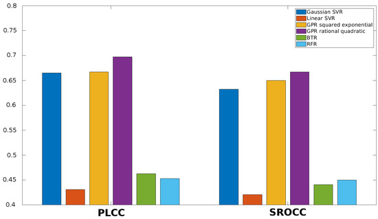
Figure 8.
Comparison of different regression methods (SVR with Gaussian kernel function, SVR with linear kernel function, GPR with squared exponential kernel function, GPR with rational quadratic kernel function, BTR, and RFR). Mean PLCC and SROCC values were measured over 20 random train-test splits on TID2013 [39].
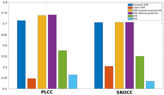
Figure 9.
Comparison of different regression methods (SVR with Gaussian kernel function, SVR with linear kernel function, GPR with squared exponential kernel function, GPR with rational quadratic kernel function, BTR, and RFR). Mean PLCC and SROCC values were measured over 20 random train-test splits on TID2008 [51].
Table 3 and Table 4 illustrate the performance of the proposed method over different distortion intensity levels and types of TID2013 [39] and TID2008 [51], respectively. From these results, it can be seen that the proposed method performs better on higher distortion levels. Furthermore, it can be seen that JPEG transmission errors, non-eccentricity pattern noise, and mean shift are very challenging distortion types, while on JPEG and JPEG2000 compressed images the proposed method achieves very high performance.
Table 3.
Average PLCC and SROCC values of the proposed method for each distortion level of TID2013 [39] and TID2008 [51].
Table 4.
Average PLCC and SROCC values of the proposed method for each distortion type of TID2013 [39] and TID2008 [51].
3.4. Comparison to the State-of-the-Art
The proposed algorithm—codenamed SPF-IQA—was compared to several state-of-the-art NR-IQA algorithms (BIQI [15], BLIINDS-II [17], BRISQUE [20], CORNIA [52], CurveletQA [26], DIIVINE [53], HOSA [54], FRIQUEE [25], GRAD-LOG-CP [23], IQVG [55], PIQE [56], SSEQ [57], and NBIQA [28]) whose original source codes are available online. These methods were re-trained using exactly the same database partition that was applied for the proposed method. As already mentioned, the used IQA database was randomly split into a training set (∼80% of images) and a test set (∼20% of images) according to the reference images. As a consequence, no semantic content overlap was between these two sets. Moreover, mean PLCC and SROCC values are reported measured over 20 random train-test splits. Besides the average PLCC and SROCC values, the statistical significance is also reported following the guidelines of [58]. As recommended in [58], the variance of z-transforms were estimated as where N stands for the number of images in a given database. Specifically, those correlation coefficients which are significantly different from SPF-IQA’s are highlighted with color in Table 5. The results of the performance comparison to the state-of-the-art on ESPL-LIVE HDR [48], KADID-10k [49], CSIQ [50], TID2013 [39], and TID2008 [51] are summarized in Table 5. From these results, it can be seen that the proposed method is able to significantly outperform the state-of-the-art on three large publicly available databases (ESPL-LIVE HDR [48], KADID-10k [49], and CSIQ [50]) in terms of PLCC and SROCC. On TID2008 [51], the proposed method is able to slightly outperform the best state-of-the-art algorithms. On TID2013 [51], SPF-IQA achieves the state-of-the-art but does not outperform the best method (FRIQUEE [25]). From Table 5, one can have another observation. SPF-IQA is superior to other state-of-the-art methods in terms of weighted PLCC and SROCC.
Table 5.
Comparison to the state-of-the-art on ESPL-LIVE HDR [48], KADID-10k [49], CSIQ [50], TID2013 [39], and TID2008 [51]. Mean PLCC and SROCC values were measured over 20 random train-test splits. The best results are typed in bold. The green background color stands for that the correlation is lower than those of the proposed method and the difference is statistically significant with p < 0.05, while the red background color means the correlation is higher and the difference is statistically significant with p < 0.05.
In Table 6, the computational times and feature vector lengths of the learning based algorithms were compared. It can be observed that the feature extraction procedure of SPF-IQA takes less than five other state-of-the-art methods (BLIINDS-II [17], DIIVINE [53], FRIQUEE [25], IQVG [55], NBIQA [28]). The computational times were measured on a personal computer containing 8-core i7-7700K CPU in MATLAB R2019a environment. On the other hand, the length of SPF-IQA’s feature vector is not significantly larger than those of other state-of-the-art methods.
Table 6.
Average feature extraction time comparison of learning-based NR-IQA methods measured on KADID-10k [49].
4. Conclusions
In this paper, the application of statistical and perceptual features was studied for no-reference image quality assessment and a novel feature extraction method was also proposed. Statistical features incorporated local fractal dimension distribution, first digit distribution in the wavelet and spatial domain, and color statistics. On the other hand, powerful perceptual features, such as colorfulness, global contrast factor, dark channel feature, entropy, and mean of phase congruency image, were also utilized. On the whole, the proposed algorithm required only 52 statistical and 5 perceptual features. In a parameter study, a wide range of regression techniques was investigated to select the one which best fits to the proposed feature vector. Finally, a Gaussian process regression (GPR) model with rational quadratic kernel function was applied to create a mapping between the feature vectors and perceptual quality scores. Experimental results on five large publicly available databases (ESPL-LIVE-HDR, KADID-10k, CSIQ, TID2013, and TID2008) showed that the proposed method is able to outperform other state-of-the-art methods.
Funding
This research received no external funding.
Acknowledgments
The author thanks the anonymous reviewers for their careful reading of the manuscript and their many insightful comments and suggestions.
Conflicts of Interest
The authors declare no conflict of interest.
References
- Dugonik, B.; Dugonik, A.; Marovt, M.; Golob, M. Image Quality Assessment of Digital Image Capturing Devices for Melanoma Detection. Appl. Sci. 2020, 10, 2876. [Google Scholar] [CrossRef]
- Kwon, H.J.; Lee, S.H. Contrast Sensitivity Based Multiscale Base–Detail Separation for Enhanced HDR Imaging. Appl. Sci. 2020, 10, 2513. [Google Scholar] [CrossRef]
- Korhonen, J. Two-level approach for no-reference consumer video quality assessment. IEEE Trans. Image Process. 2019, 28, 5923–5938. [Google Scholar] [CrossRef] [PubMed]
- Lee, C.; Cho, S.; Choe, J.; Jeong, T.; Ahn, W.; Lee, E. Objective video quality assessment. Opt. Eng. 2006, 45, 017004. [Google Scholar] [CrossRef]
- Wang, Z. Applications of objective image quality assessment methods [applications corner]. IEEE Signal Process. Mag. 2011, 28, 137–142. [Google Scholar] [CrossRef]
- Dodge, S.; Karam, L. Understanding how image quality affects deep neural networks. In Proceedings of the 2016 eighth international conference on quality of multimedia experience (QoMEX), Lisbon, Portugal, 6–8 June 2016; pp. 1–6. [Google Scholar]
- Aqqa, M.; Mantini, P.; Shah, S.K. Understanding How Video Quality Affects Object Detection Algorithms. In Proceedings of the 14th International Joint Conference on Computer Vision, Imaging and Computer Graphics Theory and Applications (VISIGRAPP 2019) (5: VISAPP), Prague, Czech Republic, 25–27 February 2019; pp. 96–104. [Google Scholar]
- Hertel, D.W.; Chang, E. Image quality standards in automotive vision applications. In Proceedings of the 2007 IEEE Intelligent Vehicles Symposium, Istanbul, Turkey, 13–15 June 2007; pp. 404–409. [Google Scholar]
- BT, R.I.R. Methodology for the Subjective Assessment of the Quality of Television Pictures; International Telecommunication Union: Bern, Switzerland, 2002; Volume 1, pp. 1–48. [Google Scholar]
- ITU-T RECOMMENDATION, P. Subjective Video Quality Assessment Methods for Multimedia Applications; International Telecommunication Union: Bern, Switzerland, 1999; Volume 1, pp. 1–42. [Google Scholar]
- Guan, J.; Zhang, W.; Gu, J.; Ren, H. No-reference blur assessment based on edge modeling. J. Vis. Commun. Image Represent. 2015, 29, 1–7. [Google Scholar] [CrossRef]
- Wang, Z.; Bovik, A.C.; Evan, B.L. Blind measurement of blocking artifacts in images. In Proceedings of the 2000 International Conference on Image Processing (Cat. No. 00CH37101), Vancouver, BC, Canada, 10–13 September 2000; Volume 3, pp. 981–984. [Google Scholar]
- Liu, H.; Klomp, N.; Heynderickx, I. A no-reference metric for perceived ringing artifacts in images. IEEE Trans. Circuits Syst. Video Technol. 2009, 20, 529–539. [Google Scholar] [CrossRef]
- Sazzad, Z.P.; Kawayoke, Y.; Horita, Y. No reference image quality assessment for JPEG2000 based on spatial features. Signal Process. Image Commun. 2008, 23, 257–268. [Google Scholar] [CrossRef]
- Moorthy, A.K.; Bovik, A.C. A two-step framework for constructing blind image quality indices. IEEE Signal Process. Lett. 2010, 17, 513–516. [Google Scholar] [CrossRef]
- Suykens, J.A.; Vandewalle, J. Least squares support vector machine classifiers. Neural Process. Lett. 1999, 9, 293–300. [Google Scholar] [CrossRef]
- Saad, M.A.; Bovik, A.C.; Charrier, C. Blind image quality assessment: A natural scene statistics approach in the DCT domain. IEEE Trans. Image Process. 2012, 21, 3339–3352. [Google Scholar] [CrossRef] [PubMed]
- Lu, P.; Li, Y.; Jin, L.; Han, S. Blind image quality assessment based on wavelet power spectrum in perceptual domain. Trans. Tianjin Univ. 2016, 22, 596–602. [Google Scholar] [CrossRef]
- Lu, W.; Zeng, K.; Tao, D.; Yuan, Y.; Gao, X. No-reference image quality assessment in contourlet domain. Neurocomputing 2010, 73, 784–794. [Google Scholar] [CrossRef]
- Mittal, A.; Moorthy, A.K.; Bovik, A.C. No-reference image quality assessment in the spatial domain. IEEE Trans. Image Process. 2012, 21, 4695–4708. [Google Scholar] [CrossRef] [PubMed]
- Drucker, H.; Burges, C.J.; Kaufman, L.; Smola, A.J.; Vapnik, V. Support vector regression machines. In Advances in Neural Information Processing Systems; MIT Press: Cambridge, MA, USA, 1997; pp. 155–161. [Google Scholar]
- Kim, D.O.; Han, H.S.; Park, R.H. Gradient information-based image quality metric. IEEE Trans. Consum. Electron. 2010, 56, 930–936. [Google Scholar] [CrossRef]
- Xue, W.; Mou, X.; Zhang, L.; Bovik, A.C.; Feng, X. Blind image quality assessment using joint statistics of gradient magnitude and Laplacian features. IEEE Trans. Image Process. 2014, 23, 4850–4862. [Google Scholar] [CrossRef]
- Liu, L.; Hua, Y.; Zhao, Q.; Huang, H.; Bovik, A.C. Blind image quality assessment by relative gradient statistics and adaboosting neural network. Signal Process. Image Commun. 2016, 40, 1–15. [Google Scholar] [CrossRef]
- Ghadiyaram, D.; Bovik, A.C. Perceptual quality prediction on authentically distorted images using a bag of features approach. J. Vis. 2017, 17, 32. [Google Scholar] [CrossRef]
- Liu, L.; Dong, H.; Huang, H.; Bovik, A.C. No-reference image quality assessment in curvelet domain. Signal Process. Image Commun. 2014, 29, 494–505. [Google Scholar] [CrossRef]
- Li, Y.; Po, L.M.; Xu, X.; Feng, L.; Yuan, F.; Cheung, C.H.; Cheung, K.W. No-reference image quality assessment with shearlet transform and deep neural networks. Neurocomputing 2015, 154, 94–109. [Google Scholar] [CrossRef]
- Ou, F.Z.; Wang, Y.G.; Zhu, G. A Novel Blind Image Quality Assessment Method Based on Refined Natural Scene Statistics. In Proceedings of the IEEE International Conference on Image Processing, Taipei, Taiwan, 22–25 September 2019; pp. 1004–1008. [Google Scholar]
- Freitas, P.G.; Akamine, W.Y.; Farias, M.C. Referenceless image quality assessment by saliency, color-texture energy, and gradient boosting machines. J. Braz. Comput. Soc. 2018, 24, 9. [Google Scholar] [CrossRef]
- Garcia Freitas, P.; Da Eira, L.P.; Santos, S.S.; Farias, M.C.Q.d. On the Application LBP Texture Descriptors and Its Variants for No-Reference Image Quality Assessment. J. Imaging 2018, 4, 114. [Google Scholar] [CrossRef]
- Mittal, A.; Soundararajan, R.; Bovik, A.C. Making a “completely blind” image quality analyzer. IEEE Signal Process. Lett. 2012, 20, 209–212. [Google Scholar] [CrossRef]
- Zhang, L.; Zhang, L.; Bovik, A.C. A feature-enriched completely blind image quality evaluator. IEEE Trans. Image Process. 2015, 24, 2579–2591. [Google Scholar] [CrossRef]
- Xue, W.; Zhang, L.; Mou, X. Learning without human scores for blind image quality assessment. In Proceedings of the IEEE Conference on Computer Vision and Pattern Recognition, Portland, OR, USA, 23–28 June 2013; pp. 995–1002. [Google Scholar]
- Mandelbrot, B.B. The Fractal Geometry of nature/Revised and Enlarged Edition; WH Freeman and Co.: New York, NY, USA, 1983; 495p. [Google Scholar]
- Al-Kadi, O.S.; Watson, D. Texture analysis of aggressive and nonaggressive lung tumor CE CT images. IEEE Trans. Biomed. Eng. 2008, 55, 1822–1830. [Google Scholar] [CrossRef]
- Fewster, R.M. A simple explanation of Benford’s Law. Am. Stat. 2009, 63, 26–32. [Google Scholar] [CrossRef]
- Al-Bandawi, H.; Deng, G. Classification of image distortion based on the generalized Benford’s law. Multimed. Tools Appl. 2019, 78, 25611–25628. [Google Scholar] [CrossRef]
- Nielsen, M. On the construction and frequency localization of finite orthogonal quadrature filters. J. Approx. Theory 2001, 108, 36–52. [Google Scholar] [CrossRef]
- Ponomarenko, N.; Jin, L.; Ieremeiev, O.; Lukin, V.; Egiazarian, K.; Astola, J.; Vozel, B.; Chehdi, K.; Carli, M.; Battisti, F.; et al. Image database TID2013: Peculiarities, results and perspectives. Signal Process. Image Commun. 2015, 30, 57–77. [Google Scholar] [CrossRef]
- Ruderman, D.L.; Cronin, T.W.; Chiao, C.C. Statistics of cone responses to natural images: Implications for visual coding. JOSA A 1998, 15, 2036–2045. [Google Scholar] [CrossRef]
- Yendrikhovskij, S.; Blommaert, F.J.; de Ridder, H. Optimizing color reproduction of natural images. In Proceedings of the Color and Imaging Conference, Scottsdale, AZ, USA, 17–20 November 1998; Society for Imaging Science and Technology: Springfield, VA, USA, 1998; Volume 1998, pp. 140–145. [Google Scholar]
- Hasler, D.; Suesstrunk, S.E. Measuring colorfulness in natural images. In Human Vision and Electronic Imaging VIII; International Society for Optics and Photonics: Bellingham, WA, USA, 2003; Volume 5007, pp. 87–95. [Google Scholar]
- Matkovic, K.; Neumann, L.; Neumann, A.; Psik, T.; Purgathofer, W. Global contrast factor—A new approach to image contrast. Comput. Aesthet. 2005, 2005, 159–168. [Google Scholar]
- He, K.; Sun, J.; Tang, X. Single image haze removal using dark channel prior. IEEE Trans. Pattern Anal. Mach. Intell. 2010, 33, 2341–2353. [Google Scholar] [PubMed]
- Kovesi, P. Phase congruency detects corners and edges. In Proceedings of the Australian Pattern Recognition Society Conference, DICTA, Sydney, Australia, 10–12 December 2003; Volume 2003. [Google Scholar]
- Morrone, M.C.; Ross, J.; Burr, D.C.; Owens, R. Mach bands are phase dependent. Nature 1986, 324, 250–253. [Google Scholar] [CrossRef]
- Qiu, W.; Chen, Y.; Kishimoto, J.; de Ribaupierre, S.; Chiu, B.; Fenster, A.; Yuan, J. Automatic segmentation approach to extracting neonatal cerebral ventricles from 3D ultrasound images. Med Image Anal. 2017, 35, 181–191. [Google Scholar] [CrossRef] [PubMed]
- Kundu, D.; Ghadiyaram, D.; Bovik, A.; Evans, B. Large-scale crowdsourced study for high dynamic range images. IEEE Trans. Image Process. 2017, 26, 4725–4740. [Google Scholar] [CrossRef]
- Lin, H.; Hosu, V.; Saupe, D. KADID-10k: A large-scale artificially distorted IQA database. In Proceedings of the 2019 Eleventh International Conference on Quality of Multimedia Experience (QoMEX), Berlin, Germany, 5–7 June 2019; pp. 1–3. [Google Scholar]
- Larson, E.C.; Chandler, D.M. Most apparent distortion: Full-reference image quality assessment and the role of strategy. J. Electron. Imaging 2010, 19, 011006. [Google Scholar]
- Ponomarenko, N.; Battisti, F.; Egiazarian, K.; Astola, J.; Lukin, V. Metrics performance comparison for color image database. In Proceedings of the Fourth International Workshop on Video Processing and Quality Metrics for Consumer Electronics, Scottsdale, AZ, USA, 14–16 January 2009; Volume 27, pp. 1–6. [Google Scholar]
- Ye, P.; Kumar, J.; Kang, L.; Doermann, D. Unsupervised feature learning framework for no-reference image quality assessment. In Proceedings of the 2012 IEEE Conference on Computer Vision and Pattern Recognition, Providence, RI, USA, 16–21 June 2012; pp. 1098–1105. [Google Scholar]
- Moorthy, A.K.; Bovik, A.C. Blind image quality assessment: From natural scene statistics to perceptual quality. IEEE Trans. Image Process. 2011, 20, 3350–3364. [Google Scholar] [CrossRef]
- Xu, J.; Ye, P.; Li, Q.; Du, H.; Liu, Y.; Doermann, D. Blind image quality assessment based on high order statistics aggregation. IEEE Trans. Image Process. 2016, 25, 4444–4457. [Google Scholar] [CrossRef]
- Gu, Z.; Zhang, L.; Li, H. Learning a blind image quality index based on visual saliency guided sampling and Gabor filtering. In Proceedings of the 2013 IEEE International Conference on Image Processing, Melbourne, Australia, 15–18 September 2013; pp. 186–190. [Google Scholar]
- Venkatanath, N.; Praneeth, D.; Bh, M.C.; Channappayya, S.S.; Medasani, S.S. Blind image quality evaluation using perception based features. In Proceedings of the 2015 Twenty First National Conference on Communications (NCC), Mumbai, India, 27 February–1 March 2015; pp. 1–6. [Google Scholar]
- Liu, L.; Liu, B.; Huang, H.; Bovik, A.C. No-reference image quality assessment based on spatial and spectral entropies. Signal Process. Image Commun. 2014, 29, 856–863. [Google Scholar] [CrossRef]
- Fieller, E.C.; Hartley, H.O.; Pearson, E.S. Tests for rank correlation coefficients. I. Biometrika 1957, 44, 470–481. [Google Scholar] [CrossRef]
© 2020 by the author. Licensee MDPI, Basel, Switzerland. This article is an open access article distributed under the terms and conditions of the Creative Commons Attribution (CC BY) license (http://creativecommons.org/licenses/by/4.0/).