A Discriminative Long Short Term Memory Network with Metric Learning Applied to Multispectral Time Series Classification


Abstract
1. Introduction
2. Methodology
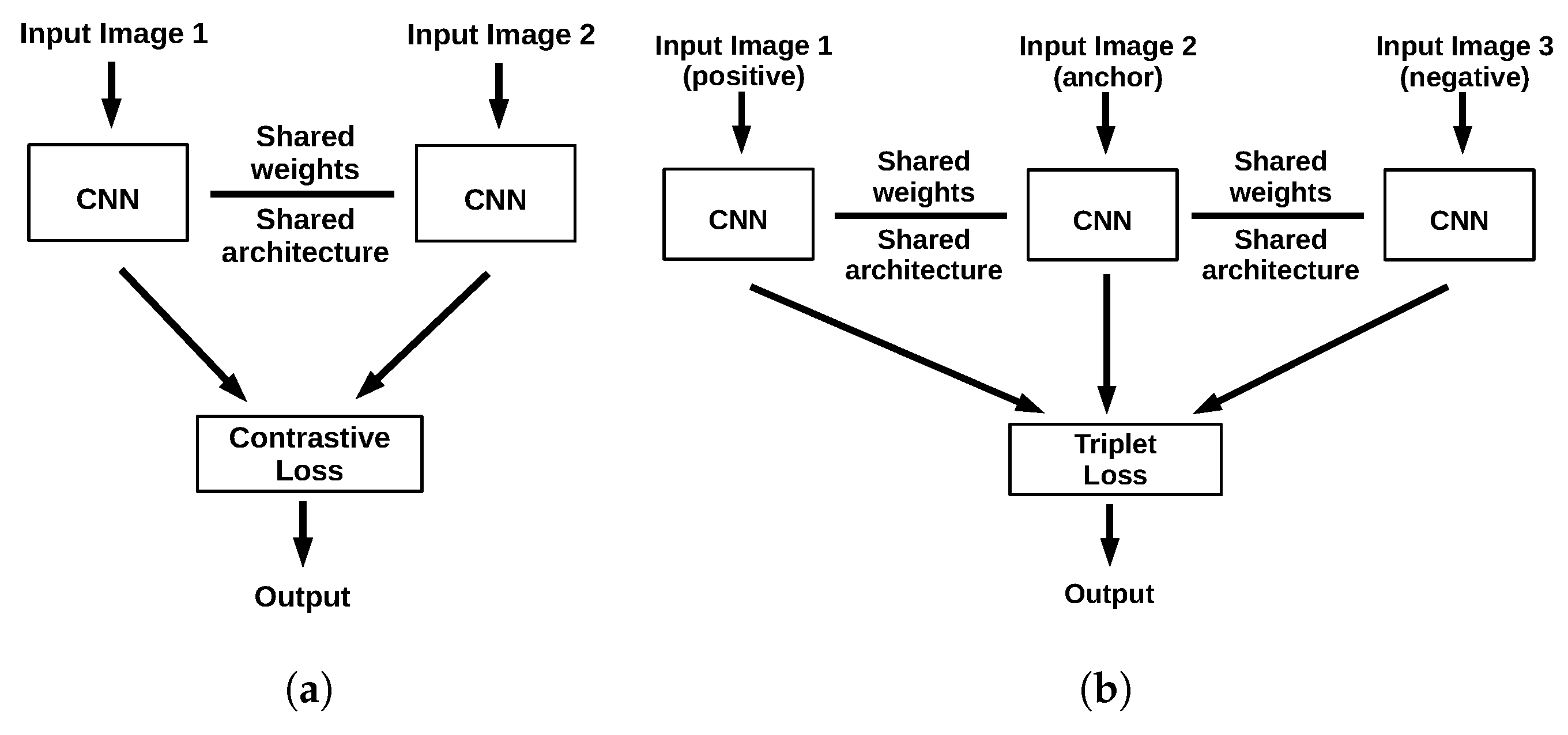
2.1. Background
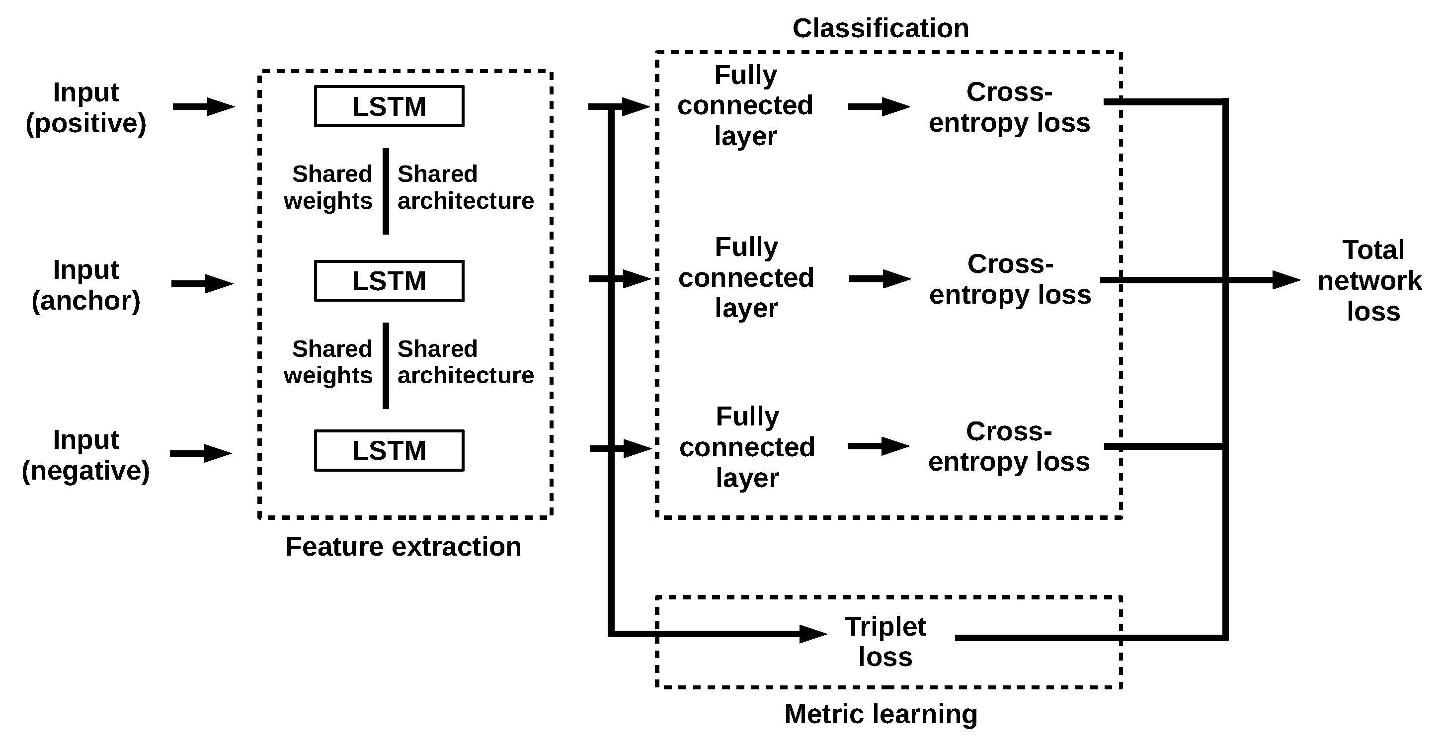
2.2. A More Discriminative LSTM
3. Experiments
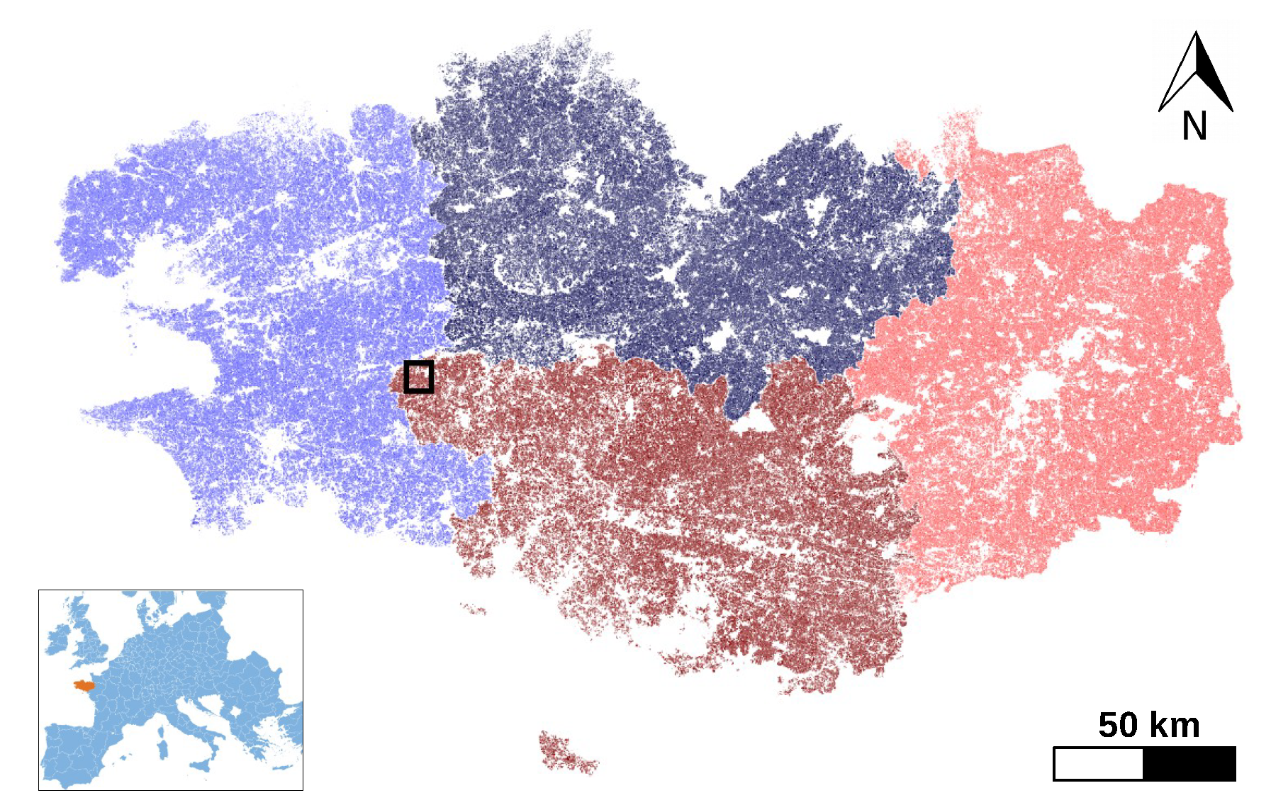
3.1. Dataset
3.2. Settings
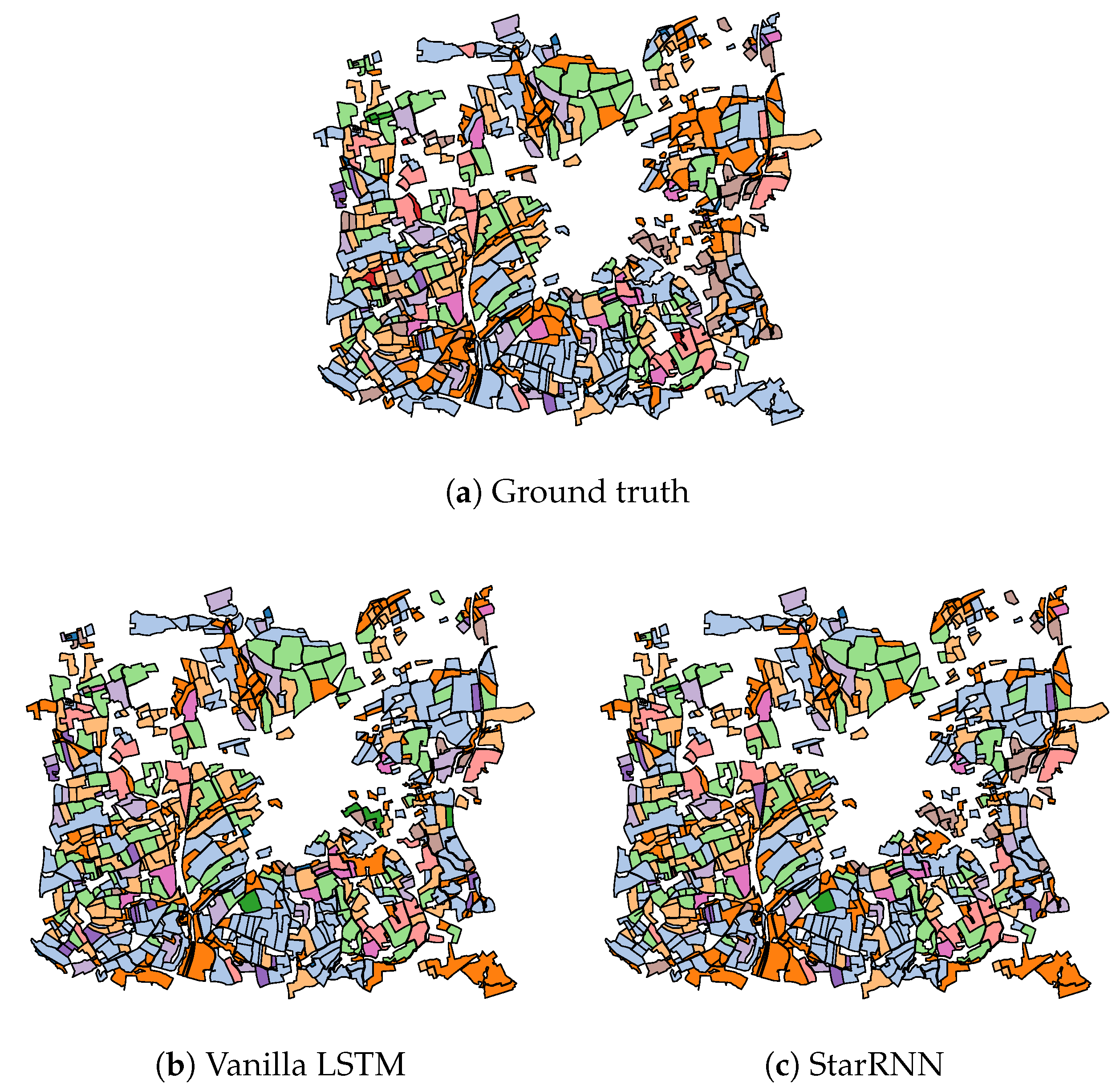
3.3. Classification Results
3.4. Computational Complexity
4. Conclusions
Author Contributions
Funding
Conflicts of Interest
References
- Belgiu, M.; Csillik, O. Sentinel-2 cropland mapping using pixel-based and object-based time-weighted dynamic time warping analysis. Remote Sens. Environ. 2018, 204, 509–523. [Google Scholar] [CrossRef]
- Gomez-Chova, L.; Tuia, D.; Moser, G.; Camps-Valls, G. Multimodal Classification of Remote Sensing Images: A Review and Future Directions. Proc. IEEE 2015, 103, 1560–1584. [Google Scholar] [CrossRef]
- Defourny, P.; Bontemps, S.; Bellemans, N.; Cara, C.; Dedieu, G.; Guzzonato, E.; Hagolle, O.; Inglada, J.; Nicola, L.; Rabaute, T. Near real-time agriculture monitoring at national scale at parcel resolution: Performance assessment of the Sen2-Agri automated system in various cropping systems around the world. Remote Sens. Environ. 2019, 221, 551–568. [Google Scholar] [CrossRef]
- Xiong, J.; Thenkabail, P.S.; Gumma, M.K.; Teluguntla, P.; Poehnelt, J.; Congalton, R.G.; Yadav, K.; Thau, D. Automated cropland mapping of continental Africa using Google EarthEngine cloud computing. Remote Sens. Environ. 2017, 126, 225–244. [Google Scholar]
- Yan, L.; Roy, D.P. Improved time series land cover classification by missing-observation-adaptive nonlinear dimensionality reduction. Remote Sens. Environ. 2015, 158, 478–491. [Google Scholar] [CrossRef]
- Solano-Correa, Y.T.; Bovolo, F.; Bruzzone, L. A Semi-supervised Crop-type Classification Based on Sentinel-2 NDVI Satellite Image Time Series and Phenological Parameters. In Proceedings of the IEEE International Geoscience and Remote Sensing Symposium, Yokohama, Japan, 28 July–2 August 2019; pp. 457–460. [Google Scholar]
- Petitjean, F.; Inglada, J.; Gancarski, P. Satellite image time series analysis under time warping. IEEE Trans. Geosci. Remote Sens. 2012, 50, 3081–3095. [Google Scholar] [CrossRef]
- Petitjean, F.; Weber, J. Efficient Satellite Image Time Series Analysis Under Time Warping. IEEE Trans. Geosci. Remote Sens. 2014, 11, 1143–1147. [Google Scholar] [CrossRef]
- Csillik, O.; Belgiu, M.; Asner, G.P.; Kelly, M. Object-Based Time-Constrained Dynamic Time Warping Classification of Crops Using Sentinel-2. Remote Sens. 2019, 11, 1257. [Google Scholar] [CrossRef]
- Furby, S.; Caccetta, P.; Wu, X.; Chia, J. Continental scale land cover change monitoring in Australia using Landsat imagery. In Proceedings of the International Earth Conference: Studying, Modeling and Sense Making of Planet Earth, Lesvos, Greece, 1–6 June 2008. [Google Scholar]
- Loveland, T.R.; Reed, B.C.; Brown, J.F.; Ohlen, D.O.; Zhu, Z.; Yang, L.; Merchant, J.W. Development of a global land cover characteristics database and IGBP DISCover from 1 km AVHRR data. Int. J. Remote Sens. 2000, 21, 1303–1330. [Google Scholar] [CrossRef]
- Zhang, Z.; Tang, P.; Corpetti, T. Satellite image time series clustering via affinity propagation. In Proceedings of the IEEE International Geoscience and Remote Sensing Symposium, Beijing, China, 10–15 July 2016. [Google Scholar]
- Gebhardt, S.; Wehrmann, T.; Muñoz Ruiz, M.A.; Maeda, P.; Bishop, J.; Schramm, M.; Kopeinig, R.; Cartus, O.; Kellndorfer, J.; Ressl, R.; et al. MAD-MEX: Automatic wall-to-wall land cover monitoring for the Mexican REDD-MRV program using all Landsat data. Remote Sens. 2014, 6, 3926–3943. [Google Scholar] [CrossRef]
- Clark, M.L.; Aide, T.M.; Rinera, G. Land change for all municipalities in Latin America and the Caribbean assessed from 250-m MODIS imagery (2001–2010). Remote Sens. Environ. 2012, 126, 84–103. [Google Scholar] [CrossRef]
- Inglada, J.; Vincent, A.; Arias, M.; Tardy, B.; Morin, D.; Rodes, I. Operational high resolution land cover map production at the country scale using satellite image time series. Remote Sens. 2017, 9, 95. [Google Scholar] [CrossRef]
- Pelletier, C.; Valero, S.; Inglada, J.; Champion, N.; Dedieu, G. Assessing the robustness of Random Forests to map land cover with high resolution satellite image time series over large areas. Remote Sens. Environ. 2016, 187, 156–168. [Google Scholar] [CrossRef]
- Gomez, C.; White, J.C.; Wulde, M.A. Optical remotely sensed time series data for land cover classification: A review. ISPRS J. Photogramm. Remote Sens. 2016, 116, 55–72. [Google Scholar] [CrossRef]
- Hinton, G.E.; Salakhutdinov, R.R. Reducing the dimensionality of data with neural networks. Science 2006, 313, 504–507. [Google Scholar] [CrossRef] [PubMed]
- Krizhevsky, A.; Sutskever, I.; Hinton, G.E. ImageNet classification with deep convolutional neural networks. In Proceedings of the International Conference on Neural Information Processing Systems, Lake Tahoe, NV, USA, 3–8 December 2012; Volume 1, pp. 1097–1105. [Google Scholar]
- Ma, L.; Liu, Y.; Zhang, X.; Ye, Y.; Yin, G.; Johnson, B.A. Deep learning in remote sensing applications: A meta-analysis and review. ISPRS J. Photogramm. Remote Sens. 2019, 152, 166–177. [Google Scholar] [CrossRef]
- Hochreiter, S.; Schmidhuber, J. Long short-term memory. Neural Comput. 1997, 9, 1735–1780. [Google Scholar] [CrossRef]
- Sun, Y.; Luo, J.; Wu, T.; Yang, Y.; Liu, H.; Dong, W.; Gao, L.; Hu, X. Geo-parcel based Crops Classification with Sentinel-1 Time Series Data via Recurrent Reural Network. In Proceedings of the IEEE International Conference on Agro-Geoinformatics, Istanbul, Turkey, 16–19 July 2019. [Google Scholar]
- Sun, Z.; Di, L.; Fang, H. Using Long Short-Term Memory Recurrent Neural Network in land cover classification on Land-sat and Cropland data layer time series. Int. J. Remote Sens. 2018, 40, 1303–1330. [Google Scholar]
- Zhong, L.; Hu, L.; Zhou, H. Deep learning based multi-temporal crop classification. Remote Sens. Environ. 2019, 221, 430–443. [Google Scholar] [CrossRef]
- Avolio, C.; Tricomi, A.; Mammone, C.; Zavagli, M.; Costantini, M. A deep learning architecture for heterogeneous and irregularly sampled remote sensing time series. In Proceedings of the IEEE International Geoscience and Remote Sensing Symposium, Yokohama, Japan, 28 July–2 August 2019. [Google Scholar]
- Garnot, V.S.F.; Landrieu, L.; Giordano, S.; Chehata, N. Time-Space Tradeoff in Deep Learning Models for Crop Classification on Satellite Multi-Spectral Image Time Series. In Proceedings of the IEEE International Geoscience and Remote Sensing Symposium, Yokohama, Japan, 28 July–2 August 2019; pp. 6247–6250. [Google Scholar]
- Zhou, Y.; Luo, J.; Fen, L.; Zhou, X. DCN-Based Spatial Features for Improving Parcel-Based Crop Classification Using High-Resolution Optical Images and Multi-Temporal SAR Data. Remote Sens. 2019, 11, 1619. [Google Scholar] [CrossRef]
- Rußwurm, M.; Körner, M. Temporal Vegetation Modelling Using Long Short-Term Memory Networks for Crop Identification from Medium-Resolution Multi-spectral Satellite Images. In Proceedings of the Computer Vision and Pattern Recognition Workshops, Honolulu, HI, USA, 21–26 July 2017; pp. 1496–1504. [Google Scholar]
- Rußwurm, M.; Körner, M. Multi-Temporal Land Cover Classification with Sequential Recurrent Encoders. ISPRS Int. J. Geo Inf. 2018, 7, 129. [Google Scholar] [CrossRef]
- Pelletier, C.; Webb, G.I.; Petitjean, F. Deep Learning for the Classification of Sentinel-2 Image Time Series. In Proceedings of the IEEE International Geoscience and Remote Sensing Symposium, Yokohama, Japan, 28 July–2 August 2019; pp. 580–583. [Google Scholar]
- Xing, E.P.; Ng, A.Y.; Jordan, M.I.; Russel, S. Distance Metric Learning, with Application to Clustering with Side-Information. In Proceedings of the International Conference on Neural Information Processing, Vancouver, BC, Canada, 9–14 December 2002; pp. 521–528. [Google Scholar]
- Tian, Z.; Zhang, Z.; Mei, S.; Jiang, R.; Wan, S.; Du, Q. Discriminative CNN via Metric Learning for Hyperspectral Classification. In Proceedings of the IEEE International Geoscience and Remote Sensing Symposium, Yokohama, Japan, 28 July–2 August 2019; pp. 580–583. [Google Scholar]
- Liu, Y.; Huang, C. Scene classification via triplet networks. IEEE J. Sel. Top. Appl. Earth Obs. Remote Sens. 2018, 11, 220–237. [Google Scholar] [CrossRef]
- Cheng, G.; Yang, C.; Yao, X.; Guo, L.; Han, J. When Deep Learning Meets Metric Learning: Remote Sensing Image Scene Classification via Learning Discriminative CNNs. IEEE Trans. Geosci. Remote Sens. 2018, 56, 2811–2821. [Google Scholar] [CrossRef]
- Liu, X.N.; Zhou, Y.; Zhao, J.Q.; Yao, R.; Liu, B.; Zheng, Y. Siamese Convolutional Neural Networks for Remote Sensing Scene Classification. IEEE Trans. Geosci. Remote Sens. 2019, 16, 1200–1204. [Google Scholar] [CrossRef]
- Bromley, J.; Guyon, I.; LeCun, Y.; Säckinger, E.; Shah, R. Signature Verification using a “Siamese” Time Delay Neural Network. In Proceedings of the Conference on Neural Information Processing Systems, Denver, CO, USA, 29 November–2 December 1993; pp. 737–744. [Google Scholar]
- Zhan, Y.; Fu, K.; Yan, M.; Sun, X.; Wang, H.; Qiu, X. Change Detection Based on Deep Siamese Convolutional Network for Optical Aerial Images. IEEE Trans. Geosci. Remote Sens. 2017, 14, 1845–1849. [Google Scholar] [CrossRef]
- Chopra, S.; Hadsell, R.; LeCun, Y. Learning a similarity metric discriminatively, with application to face verification. In Proceedings of the IEEE Conference on Computer Vision and Pattern Recognition, San Diego, CA, USA, 20–25 June 2005; pp. 539–546. [Google Scholar]
- Hoffer, E.; Ailon, N. Deep Metric Learning Using Triplet Network. In Proceedings of the International Workshop on Similarity-Based Pattern Recognition, Copenhagen, Denmark, 12–14 October 2015; pp. 84–92. [Google Scholar]
- Rußwurm, M.; Lefèvre, S.; Körner, M. BreizhCrops: A Time Series Dataset for Crop Type Identification. In Proceedings of the Time Series Workshop of the 36th International Conference on Machine Learning, Long Beach, CA, USA, 10–15 June 2019. [Google Scholar]
- Bosilj, P.; Aptoula, E.; Duckett, T.; Cielniak, G. Transfer learning between crop types for semantic segmentation of crops versus weeds in precision agriculture. J. Field Robot. 2020, 37, 7–19. [Google Scholar] [CrossRef]
- Eigen, D.; Fergus, R. Predicting depth, surface normals and semantic labels with a common multi-scale convolutional architecture. In Proceedings of the IEEE International Conference on Computer Vision, Las Condes, Chile, 11–18 December 2015; pp. 2650–2658. [Google Scholar]
- Rußwurm, M.; Pelletier, C.; Zollner, M.; Lefèvre, S.; Körner, M. BreizhCrops: A Time Series Dataset for Crop Type Mapping. arXiv 2020, arXiv:1905.11893v2. [Google Scholar]
- Kingma, D.; Ba, J. Adam: A method for stochastic optimization. In Proceedings of the International Conference on Learning Representation, San Diego, CA, USA, 7–9 May 2015. [Google Scholar]
- Turkoglu, M.O.; D’Aronco, S.; Wegner, J.D.; Schindler, K. Gating Revisited: Deep Multi-layer RNNs That Can BeTrained. arXiv 2019, arXiv:1911.11033. [Google Scholar]
- Pahlevan, N.; Smith, B.; Schalles, J.; Binding, C.; Cao, Z.; Mae, R.; Alikas, K.; Kangrof, K.; Gurling, D.; Hà, N.; et al. Seamless retrievals of chlorophyll-a from Sentinel-2 (MSI) and Sentinel-3 (OLCI) in inland and coastal waters: A machine-learning approach. Remote Sens. Environ. 2020, 240, 111604. [Google Scholar] [CrossRef]
- Ienco, D.; Gaetano, R.; Dupaquier, C.; Maurel, P. Land Cover Classification via Multitemporal Spatial Data by Deep Recurrent Neural Networks. IEEE Trans. Geosci. Remote Sens. 2017, 14, 1685–1689. [Google Scholar] [CrossRef]
- Kussul, N.; Lavreniuk, M.; Skakun, S.; Shelestov, A. Deep learning classification of land cover and crop types using remote sensing data. IEEE Trans. Geosci. Remote Sens. 2017, 14, 778–782. [Google Scholar] [CrossRef]


| Class # | Crop Type | FRH01 | FRH02 | FRH03 | FRH04 |
|---|---|---|---|---|---|
| 1 | barley | 13,046 | 10,733 | 7148 | 5978 |
| 2 | wheat | 30,368 | 15,005 | 27,189 | 16,993 |
| 3 | corn | 43,990 | 36,593 | 41,992 | 31,333 |
| 4 | fodder | 6514 | 4329 | 7639 | 4541 |
| 5 | fallow | 1521 | 3267 | 2814 | 4555 |
| 6 | miscellaneous | 17,659 | 12,126 | 21,194 | 15,571 |
| 7 | orchards | 944 | 350 | 1223 | 553 |
| 8 | cereals | 6276 | 3660 | 4516 | 5784 |
| 9 | perm. meadows | 32,650 | 36,512 | 32,534 | 26,117 |
| 10 | protein crops | 1107 | 461 | 1079 | 655 |
| 11 | rapeseed | 5593 | 2346 | 3557 | 3236 |
| 12 | temp. meadows | 52,011 | 39,082 | 52,728 | 38,391 |
| 13 | vegetables | 8538 | 14,266 | 3679 | 3851 |
| Total | 220,217 | 178,730 | 207,292 | 157,558 |
| Method | OA | Mean f1 | Mean Precision | Mean Recall | |
|---|---|---|---|---|---|
| Random Forest | 0.545 | 0.441 | 0.295 | 0.339 | 0.312 |
| Temporal CNN | 0.624 | 0.546 | 0.440 | 0.554 | 0.440 |
| MsResNet | 0.632 | 0.565 | 0.502 | 0.658 | 0.491 |
| InceptionNet | 0.632 | 0.570 | 0.535 | 0.591 | 0.533 |
| StarRNN | 0.664 | 0.596 | 0.529 | 0.582 | 0.530 |
| Vanilla LSTM [40] | 0.680 | 0.620 | 0.590 | 0.630 | 0.580 |
| TripletLSTM-1 | 0.711 | 0.641 | 0.631 | 0.642 | 0.620 |
| TripletLSTM-2 | 0.678 | 0.619 | 0.588 | 0.590 | 0.604 |
| Method | Training Duration | Number of Network Parameters |
|---|---|---|
| Random Forest | 39 | - |
| Temporal CNN | 36 | 787,085 |
| MsResNet | 30 | 537,325 |
| InceptionNet | 37 | 215,053 |
| StarRNN | 39 | 72,103 |
| Vanilla LSTM [40] | 33 | 942,376 |
| TripletLSTM-1 | 39 | 942,375 |
| TripletLSTM-2 | 37 | 942,375 |
© 2020 by the authors. Licensee MDPI, Basel, Switzerland. This article is an open access article distributed under the terms and conditions of the Creative Commons Attribution (CC BY) license (http://creativecommons.org/licenses/by/4.0/).
Share and Cite
Bozo, M.; Aptoula, E.; Çataltepe, Z. A Discriminative Long Short Term Memory Network with Metric Learning Applied to Multispectral Time Series Classification. J. Imaging 2020, 6, 68. https://doi.org/10.3390/jimaging6070068
Bozo M, Aptoula E, Çataltepe Z. A Discriminative Long Short Term Memory Network with Metric Learning Applied to Multispectral Time Series Classification. Journal of Imaging. 2020; 6(7):68. https://doi.org/10.3390/jimaging6070068
Chicago/Turabian StyleBozo, Merve, Erchan Aptoula, and Zehra Çataltepe. 2020. "A Discriminative Long Short Term Memory Network with Metric Learning Applied to Multispectral Time Series Classification" Journal of Imaging 6, no. 7: 68. https://doi.org/10.3390/jimaging6070068
APA StyleBozo, M., Aptoula, E., & Çataltepe, Z. (2020). A Discriminative Long Short Term Memory Network with Metric Learning Applied to Multispectral Time Series Classification. Journal of Imaging, 6(7), 68. https://doi.org/10.3390/jimaging6070068