Further Improvement of Debayering Performance of RGBW Color Filter Arrays Using Deep Learning and Pansharpening Techniques


Abstract
1. Introduction
- We are the first team to propose the combination of pansharpening and deep learning to demosaic RGBW pattern. Our approach opens a new direction in this research field and may stimulate more research in this area;
- Our new results improved over our earlier results in [4];
2. Enhanced Pansharpening Approach to Demosaicing of RGBW CFAs
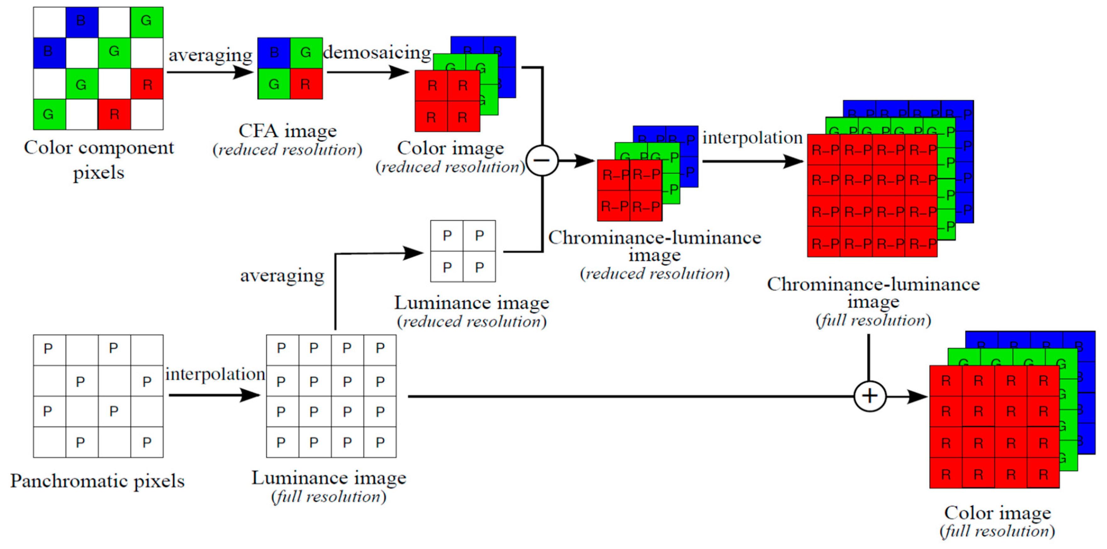
2.1. Standard Approach
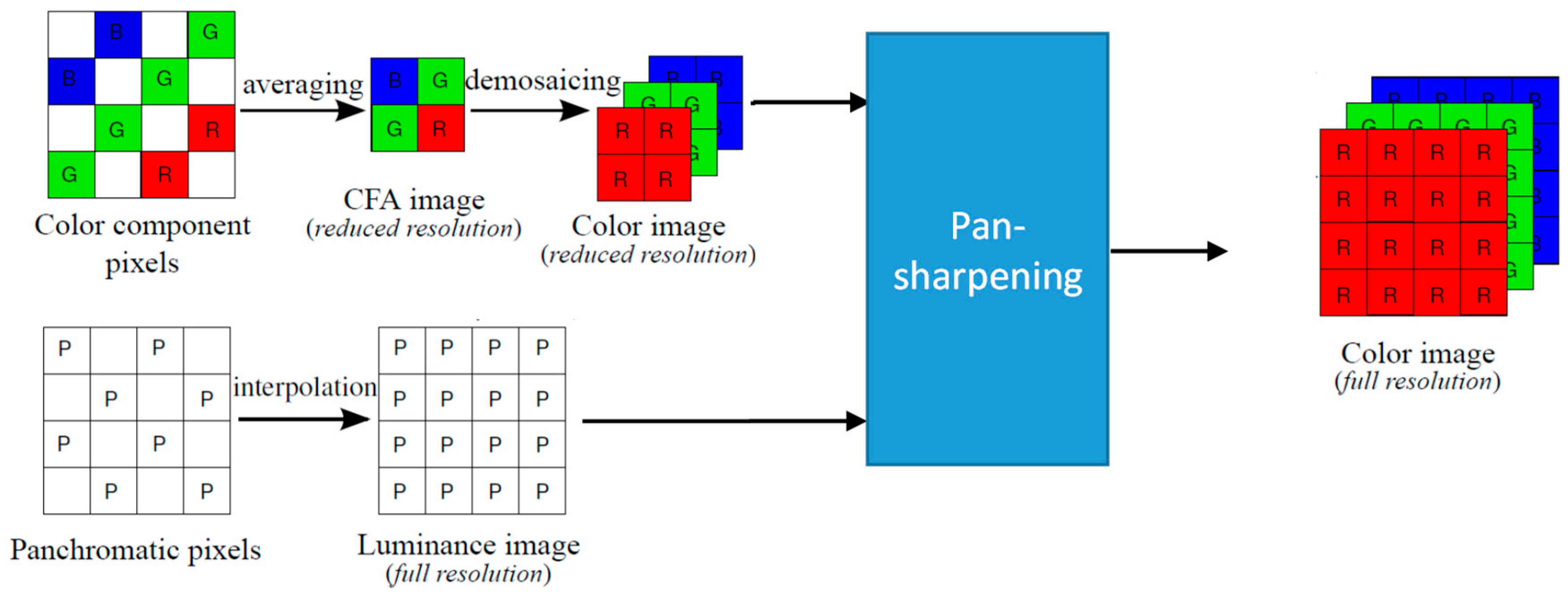
2.2. Pansharpening Approach to Denosaicing CFA2.0 Patterns
2.3. Enhanced Pansharpening Approach
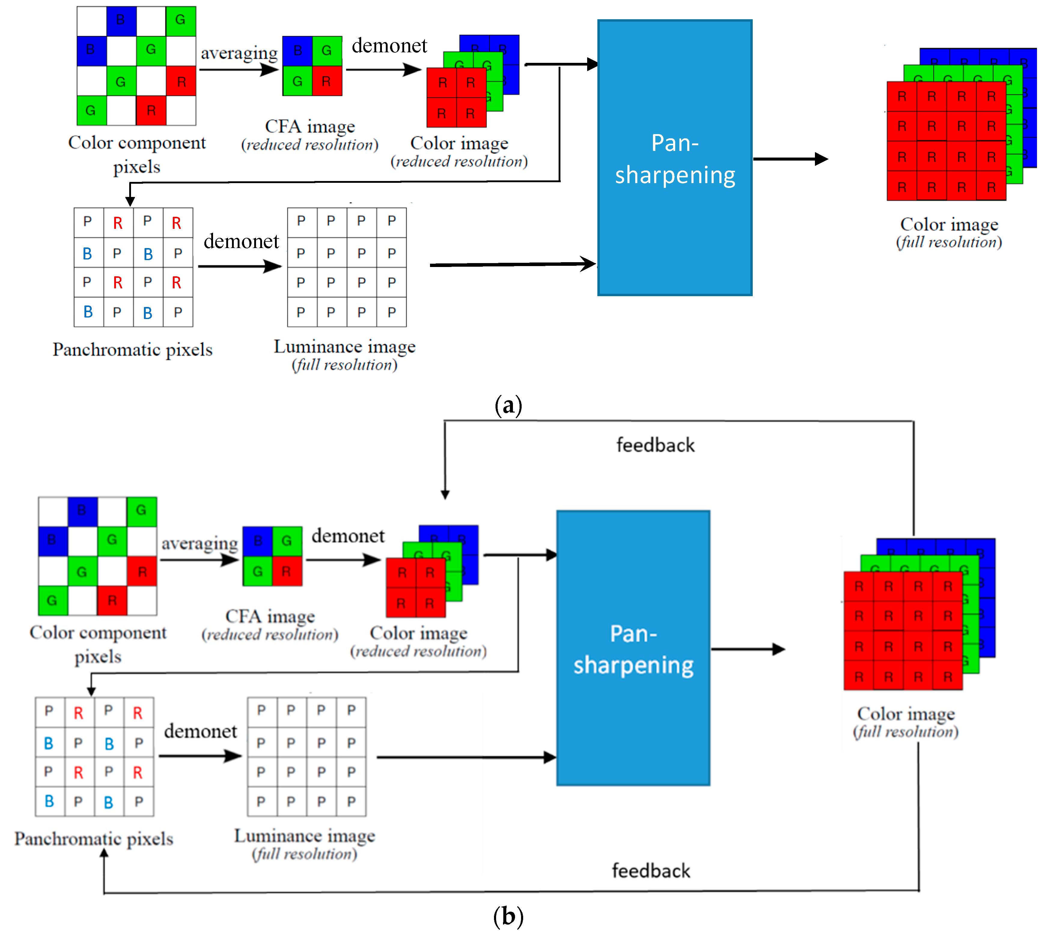
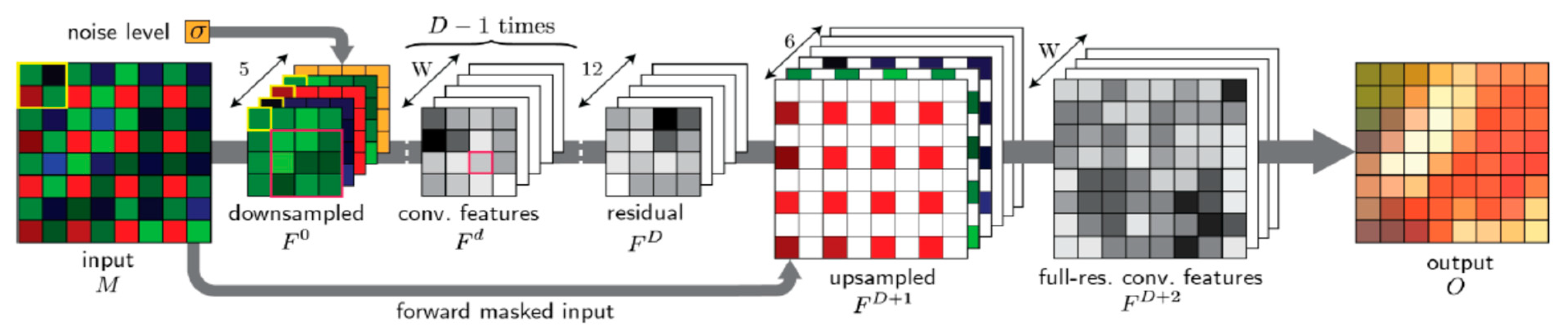
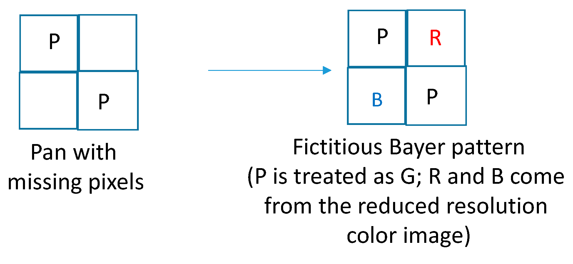
- First, we will explain how DEMONET was used for improving the pan band. Our idea was motivated by the research of [36] in which it was observed that the white (W) channel has a higher spectral correlation with the R and B channels than the G channel. Hence, we create a fictitious Bayer pattern where the original W (also known as P) pixels are treated as G pixels, the missing W pixels are filled in with interpolated R and B pixels from the low resolution RGB image. Figure 6 illustrates the creation of the fictitious Bayer pattern.
- Second, we would like to emphasize that we did not re-train the DEMONET because we do not have that many images. Most importantly, the DEMONET was trained with millions of diverse images. The performance of the above way of generating the pan band is quite good, as can be seen from Table 1;
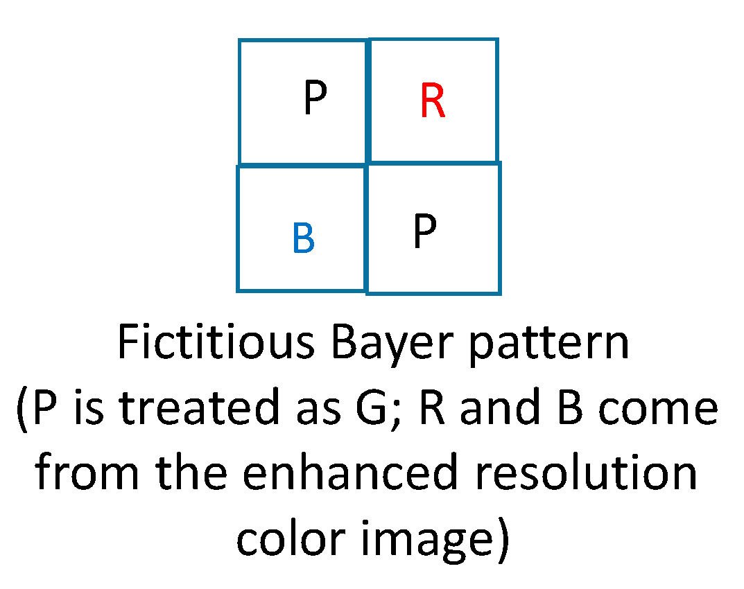
- Third, we will explain how feedback works. There are two feedback paths. After the first iteration, we will obtain an enhanced color image. In the first feedback path, we replace the reduced resolution color image in Figure 4 with a downsized version of the enhanced color image. In the second feedback path, we directly replace the R and B pixels with the corresponding R and B pixels from the enhanced color image as shown in Figure 7.
| Combined Deep Learning and Pansharpening for Demosaicing RGBW Patterns |
| Input: An RGBW pattern |
| Output: A demosaiced color image |
| I = 1; iteration number |
|
| * I = I + 1 |
| If I > K, then stop. K is a pre-designed integer. We used K = 3 in our experiments. |
| Otherwise, |
|
| Go to * |
3. Experimental Results
3.1. Data: IMAX and Kodak
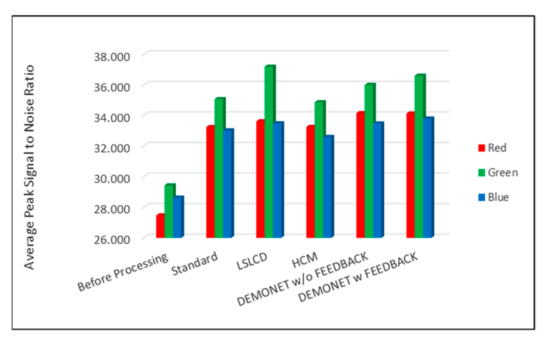
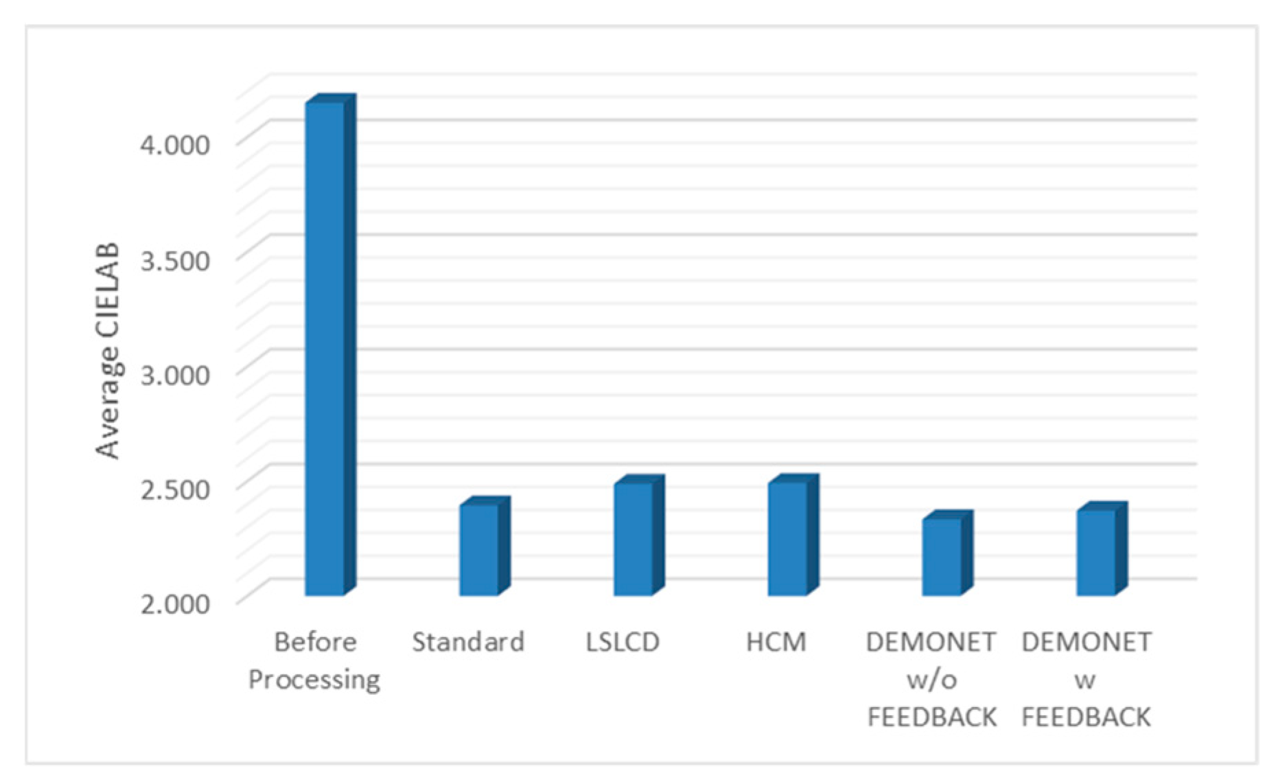
3.2. Performance Metrics and Comparison of Different Approaches to Generating the Pan Band
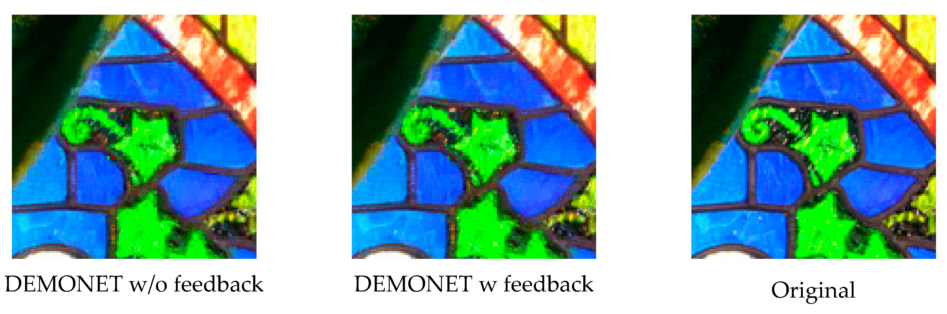
3.3. Evaluation Using IMAX Images
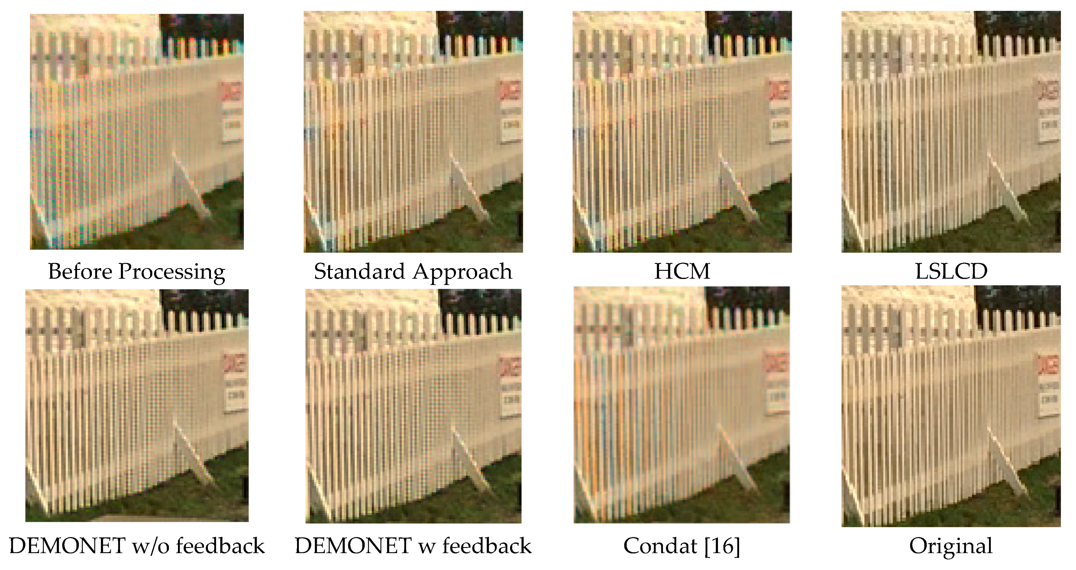
3.4. Evaluation Using Kodak Images
4. Conclusions
Author Contributions
Funding
Conflicts of Interest
References
- Bayer, B.E. Color Imaging Array. U.S. Patent 3,971,065, 20 July 1976. [Google Scholar]
- Losson, O.; Macaire, L.; Yang, Y. Comparison of color demosaicing methods. Adv. Imaging Electron Phys. Elsevier 2010, 162, 173–265. [Google Scholar]
- Kijima, T.; Nakamura, H.; Compton, J.T.; Hamilton, J.F.; DeWeese, T.E. Image Sensor With Improved Light Sensitivity. U.S. Patent US 8,139,130, 20 March 2012. [Google Scholar]
- Kwan, C.; Chou, B.; Kwan, L.M.; Budavari, B. Debayering RGBW color filter arrays: A pansharpening approach. In Proceedings of the IEEE Ubiquitous Computing, Electronics & Mobile Communication Conference, New York, NY, USA, 19–21 October 2017; pp. 94–100. [Google Scholar]
- Zhang, L.; Wu, X.; Buades, A.; Li, X. Color demosaicking by local directional interpolation and nonlocal adaptive thresholding. J. Electron. Imaging 2011, 20, 023016. [Google Scholar]
- Malvar, H.S.; He, L.-W.; Cutler, R. High-quality linear interpolation for demosaciking of color images. IEEE Int. Conf. Acoust. Speech Signal Process. 2004, 3, 485–488. [Google Scholar]
- Lian, N.-X.; Chang, L.; Tan, Y.-P.; Zagorodnov, V. Adaptive filtering for color filter array demosaicking. IEEE Trans. Image Process. 2007, 16, 2515–2525. [Google Scholar] [CrossRef] [PubMed]
- Kwan, C.; Chou, B.; Kwan, L.M.; Larkin, J.; Ayhan, B.; Bell, J.F.; Kerner, H. Demosaicking enhancement using pixel level fusion. J. Signal Image Video Process. 2018, 12, 749–756. [Google Scholar] [CrossRef]
- Zhang, L.; Wu, X. Color demosaicking via directional linear minimum mean square-error estimation. IEEE Trans. IP 2005, 14, 2167–2178. [Google Scholar] [CrossRef]
- Lu, W.; Tan, Y.P. Color filter array demosaicking: New method and performance measures. IEEE Trans. IP 2003, 12, 1194–1210. [Google Scholar]
- Dubois, E. Frequency-domain methods for demosaicking of bayer-sampled color images. IEEE Signal Proc. Lett. 2005, 12, 847–850. [Google Scholar] [CrossRef]
- Gunturk, B.; Altunbasak, Y.; Mersereau, R.M. Color plane interpolation using alternating projections. IEEE Trans. Image Process. 2002, 11, 997–1013. [Google Scholar] [CrossRef]
- Rafinazaria, M.; Dubois, E. Demosaicking algorithm for the Kodak-RGBW color filter array. In Proceedings of the Color Imaging XX: Displaying, Processing, Hardcopy, and Applications, San Francisco, CA, USA, 9–12 February 2015; Volume 9395. [Google Scholar]
- Leung, B.; Jeon, G.; Dubois, E. Least-squares luma-chroma demultiplexing algorithm for Bayer demosaicking. IEEE Trans. Image Process. 2011, 20, 1885–1894. [Google Scholar] [CrossRef]
- Zhang, C.; Li, Y.; Wang, J.; Hao, P. Universal demosaicking of color filter arrays. IEEE Trans. Image Process. 2016, 25, 5173–5186. [Google Scholar] [CrossRef] [PubMed]
- Condat, L. A generic variational approach for demosaicking from an arbitrary color filter array. In Proceedings of the IEEE International Conference on Image Processing (ICIP), Cairo, Egypt, 7–10 November 2009; pp. 1625–1628. [Google Scholar]
- Menon, D.; Calvagno, G. Regularization approaches to demosaicking. IEEE Trans. Image Process. 2009, 18, 2209–2220. [Google Scholar] [CrossRef] [PubMed]
- Li, J.; Bai, C.; Lin, Z.; Yu, J. Automatic design of high-sensitivity color filter arrays with panchromatic pixels. IEEE Trans. Image Process. 2017, 26, 870–883. [Google Scholar] [CrossRef] [PubMed]
- Zhou, J.; Kwan, C.; Budavari, B. Hyperspectral image super-resolution: A hybrid color mapping approach. Appl. Remote Sens. 2016, 10, 035024. [Google Scholar] [CrossRef]
- Kwan, C.; Choi, J.; Chan, S.; Zhou, J.; Budavari, B. A Super-Resolution and fusion approach to enhancing hyperspectral images. Remote Sens. 2018, 10, 1416. [Google Scholar] [CrossRef]
- Kwan, C.; Budavari, B.; Feng, G. A hybrid color mapping approach to fusing MODIS and Landsat images for forward prediction. Remote Sens. 2017, 10, 520. [Google Scholar] [CrossRef]
- Ayhan, B.; Dao, M.; Kwan, C.; Chen, H.; Bell, J.F., III; Kidd, R. A novel utilization of image registration techniques to process Mastcam images in Mars rover with applications to image fusion, pixel clustering, and anomaly detection. IEEE J. Sel. Top. Appl. Earth Obs. Remote Sens. 2017, 10, 4553–4564. [Google Scholar] [CrossRef]
- Kwan, C.; Budavari, B.; Bovik, A.; Marchisio, G. Blind quality assessment of fused WorldView-3 images by using the combinations of pansharpening and hypersharpening paradigms. IEEE Geosci. Remote Sens. Lett. 2017, 14, 1835–1839. [Google Scholar] [CrossRef]
- Qu, Y.; Qi, H.; Ayhan, B.; Kwan, C.; Kidd, R. Does multispectral/hyperspectral pansharpening improve the performance of anomaly detection? In Proceedings of the IEEE International Geoscience and Remote Sensing Symposium, Fort Worth, TX, USA, 23–28 July 2017, pp. 6130–6133. [Google Scholar]
- Chavez, P.S., Jr.; Sides, S.C.; Anderson, J.A. Comparison of three different methods to merge multiresolution and multispectral data: Landsat TM and SPOT panchromatic. Photogramm. Eng. Remote Sens. 1991, 57, 295–303. [Google Scholar]
- Vivone, G.; Alparone, L.; Chanussot, J.; Mura, M.D.; Garzelli, A.; Licciardi, G.; Restaino, R.; Wald, L. A critical comparison among pansharpening algorithms. IEEE Trans. Geosci. Remote Sens. 2015, 53, 2565–2586. [Google Scholar] [CrossRef]
- Liu, J.G. Smoothing filter based intensity modulation: A spectral preserve image fusion technique for improving spatial details. Int. J. Remote Sens. 2000, 21, 3461–3472. [Google Scholar] [CrossRef]
- Aiazzi, B.; Alparone, L.; Baronti, S.; Garzelli, A.; Selva, M. MTF-tailored multiscale fusion of high-resolution MS and pan imagery. Photogramm. Eng. Remote Sens. 2006, 72, 591–596. [Google Scholar] [CrossRef]
- Vivone, G.; Restaino, R.; Mauro, D.M.; Licciardi, G.; Chanussot, J. Contrast and error-based fusion schemes for multispectral image pansharpening. IEEE Trans. Geosci. Remote Sens. Lett. 2014, 11, 930–934. [Google Scholar] [CrossRef]
- Laben, C.; Brower, B. Process for Enhancing the Spatial Resolution of Multispectral Imagery Using Pan-Sharpening. U.S. Patent 6,011,875, 4 January 2000. [Google Scholar]
- Aiazzi, B.; Baronti, S.; Selva, M. Improving component substitution pansharpening through multivariate regression of MS+pan data. IEEE Trans. Geosci. Remote Sens. 2007, 45, 3230–3239. [Google Scholar] [CrossRef]
- Liao, W.; Huang, X.; Coillie, F.V.; Gautama, S.; Pižurica, A.; Liu, H.; Philips, W.; Zhu, T.; Shimoni, M.; Moser, G.; et al. Processing of multiresolution thermal hyperspectral and digital color data: Outcome of the 2014 IEEE GRSS data fusion contest. IEEE J. Select. Top. Appl. Earth Observ. Remote Sens. 2015, 8, 2984–2996. [Google Scholar] [CrossRef]
- Choi, J.; Yu, K.; Kim, Y. A new adaptive component-substitution based satellite image fusion by using partial replacement. IEEE Trans. Geosci. Remote Sens. 2011, 49, 2984–2996. [Google Scholar] [CrossRef]
- Hybrid Color Mapping (HCM) Codes. Available online: https://openremotesensing.net/knowledgebase/hyperspectral-image-superresolution-a-hybrid-color-mapping-approach/ (accessed on 22 December 2018).
- Gharbi, M.; Chaurasia, G.; Paris, S.; Durand, F. Deep joint demosaicking and denoising. Acm. Trans. Graph. 2016, 35, 191. [Google Scholar] [CrossRef]
- Oh, L.S.; Kang, M.G. Colorization-based rgb-white color interpolation using color filter array with randomly sampled pattern. Sensors 2017, 17, 1523. [Google Scholar] [CrossRef]
- Zhang, X.; Wandell, B.A. A spatial extension of cielab for digital color image reproduction. SID J. 1997, 5, 61–63. [Google Scholar]


| Interpolation Method | PSNR |
|---|---|
| BILINEAR | 31.2574 |
| Malvar-He-Cutler (MHC) | 31.9133 |
| DEMONET using R and B pixels from the Reduced resolution RGB | 33.1281 |
| DEMONET using R and B pixels from the GROUND TRUTH RGB image | 37.4825 |
| Image | Metric | Before Processing | Standard | LSLCD | HCM | DEMONET w/o FEEDBACK | DEMONET w FEEDBACK |
|---|---|---|---|---|---|---|---|
| 1 | PSNR | 23.965 | 26.203 | 24.648 | 26.210 | 25.783 | 26.182 |
| CIELAB | 9.447 | 8.182 | 9.611 | 7.755 | 7.897 | 7.682 | |
| 2 | PSNR | 28.879 | 32.812 | 31.594 | 32.354 | 32.010 | 32.759 |
| CIELAB | 6.384 | 5.459 | 6.524 | 5.105 | 5.053 | 4.858 | |
| 3 | PSNR | 24.390 | 28.917 | 29.563 | 28.880 | 29.026 | 30.085 |
| CIELAB | 8.777 | 6.400 | 6.833 | 5.806 | 6.028 | 5.635 | |
| 4 | PSNR | 26.838 | 31.528 | 31.699 | 32.980 | 32.386 | 34.061 |
| CIELAB | 3.887 | 2.723 | 2.935 | 2.101 | 2.286 | 2.080 | |
| 5 | PSNR | 27.709 | 30.433 | 28.937 | 31.460 | 30.968 | 31.503 |
| CIELAB | 5.087 | 4.107 | 5.073 | 3.753 | 4.073 | 3.901 | |
| 6 | PSNR | 31.355 | 32.866 | 30.795 | 33.715 | 33.538 | 33.999 |
| CIELAB | 4.530 | 3.995 | 5.014 | 3.600 | 3.705 | 3.583 | |
| 7 | PSNR | 28.637 | 33.545 | 34.391 | 32.293 | 33.547 | 34.786 |
| CIELAB | 5.045 | 3.340 | 3.484 | 3.654 | 2.991 | 2.836 | |
| 8 | PSNR | 29.614 | 34.583 | 34.438 | 34.239 | 34.610 | 36.118 |
| CIELAB | 6.441 | 5.235 | 6.394 | 5.198 | 5.101 | 4.884 | |
| 9 | PSNR | 30.964 | 34.298 | 32.133 | 34.899 | 33.962 | 34.869 |
| CIELAB | 4.867 | 4.325 | 5.561 | 3.584 | 3.474 | 3.304 | |
| 10 | PSNR | 32.068 | 35.430 | 33.407 | 34.996 | 34.982 | 35.518 |
| CIELAB | 5.191 | 4.458 | 5.754 | 4.076 | 4.198 | 4.038 | |
| 11 | PSNR | 33.733 | 36.475 | 34.332 | 36.364 | 36.654 | 37.203 |
| CIELAB | 5.523 | 5.159 | 6.704 | 4.206 | 4.043 | 3.893 | |
| 12 | PSNR | 29.501 | 34.629 | 34.493 | 34.982 | 35.126 | 36.358 |
| CIELAB | 4.289 | 3.091 | 3.700 | 2.886 | 2.908 | 2.697 | |
| 13 | PSNR | 34.374 | 38.003 | 36.480 | 38.686 | 38.542 | 39.245 |
| CIELAB | 2.285 | 1.825 | 2.186 | 1.729 | 1.760 | 1.705 | |
| 14 | PSNR | 33.535 | 36.651 | 35.852 | 36.826 | 36.545 | 37.080 |
| CIELAB | 3.784 | 3.357 | 3.919 | 3.175 | 3.224 | 3.147 | |
| 15 | PSNR | 34.716 | 37.254 | 35.470 | 37.610 | 37.010 | 37.641 |
| CIELAB | 4.208 | 3.992 | 5.306 | 3.586 | 3.805 | 3.677 | |
| 16 | PSNR | 27.638 | 29.756 | 28.101 | 31.011 | 30.811 | 31.567 |
| CIELAB | 9.417 | 8.560 | 9.837 | 6.578 | 6.053 | 5.793 | |
| 17 | PSNR | 28.159 | 29.222 | 26.304 | 28.806 | 28.528 | 28.927 |
| CIELAB | 9.477 | 9.381 | 12.852 | 8.330 | 8.329 | 8.111 | |
| 18 | PSNR | 28.113 | 33.122 | 31.152 | 32.376 | 32.857 | 33.840 |
| CIELAB | 6.270 | 4.808 | 5.475 | 4.368 | 3.828 | 3.636 | |
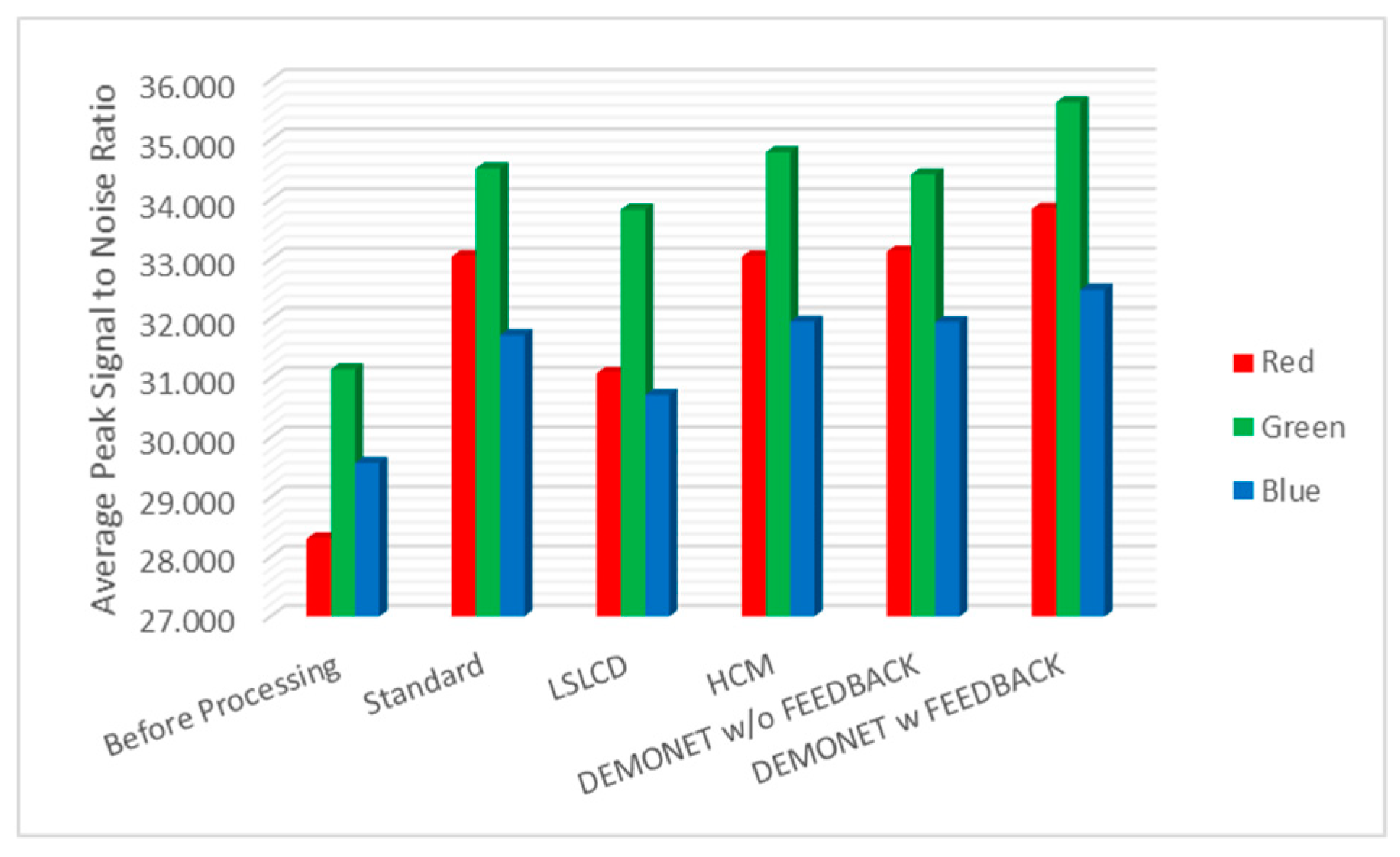
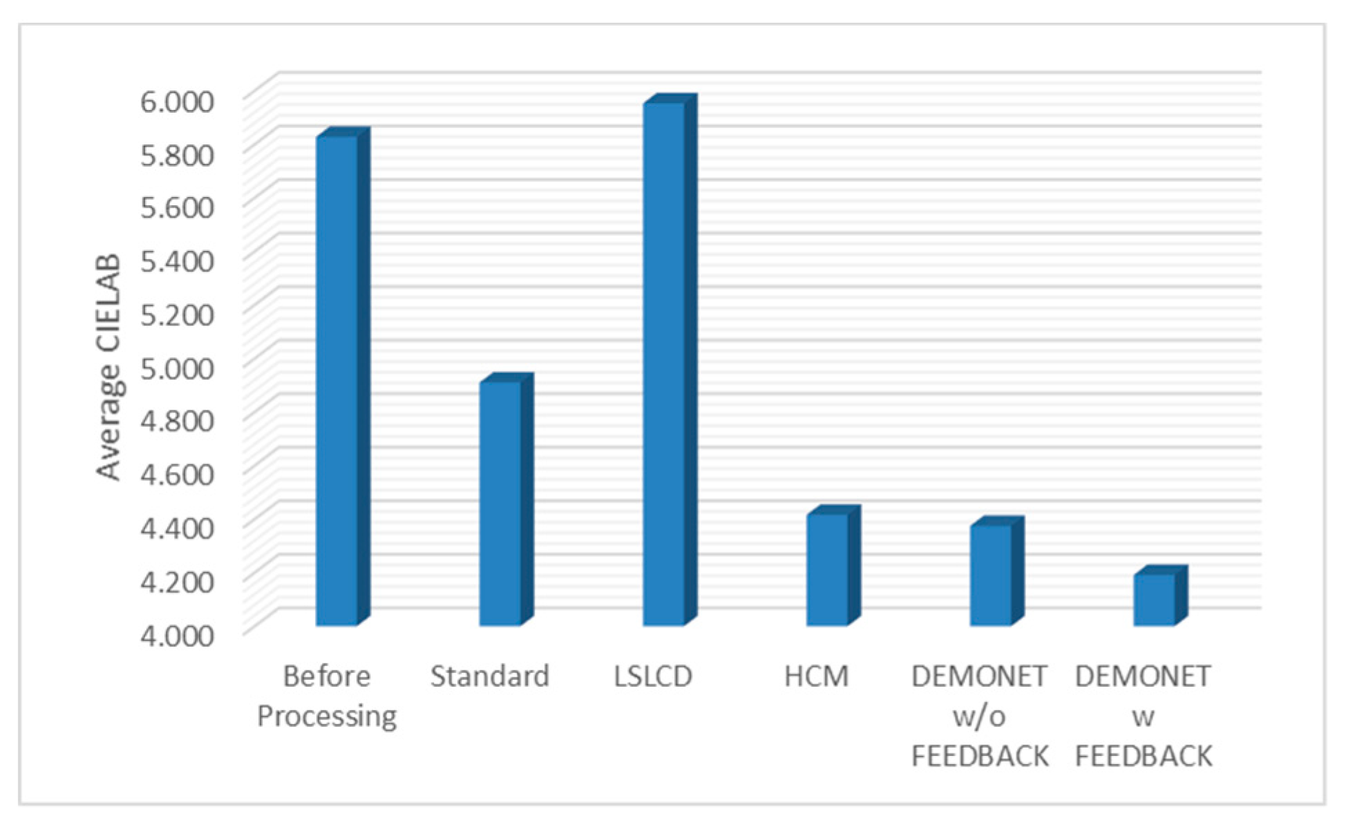
| Average | PSNR | 29.677 | 33.096 | 31.877 | 33.260 | 33.160 | 33.986 |
| CIELAB | 5.828 | 4.911 | 5.954 | 4.416 | 4.375 | 4.192 |
| Image | Metric | Before Processing | Standard | LSLCD | HCM | DEMONET w/o FEEDBACK | DEMONET w FEEDBACK |
|---|---|---|---|---|---|---|---|
| 1 | PSNR | 33.018 | 37.560 | 32.111 | 37.095 | 37.994 | 37.986 |
| CIELAB | 2.123 | 1.534 | 3.646 | 1.632 | 1.623 | 1.657 | |
| 2 | PSNR | 26.305 | 31.862 | 36.086 | 31.756 | 33.306 | 33.827 |
| CIELAB | 4.869 | 2.719 | 2.022 | 2.820 | 2.485 | 2.518 | |
| 3 | PSNR | 31.690 | 36.777 | 34.484 | 36.180 | 36.433 | 36.616 |
| CIELAB | 2.936 | 1.877 | 2.831 | 2.103 | 2.155 | 2.198 | |
| 4 | PSNR | 22.690 | 29.447 | 31.288 | 29.536 | 30.780 | 31.439 |
| CIELAB | 7.593 | 3.608 | 3.343 | 3.608 | 3.211 | 3.196 | |
| 5 | PSNR | 30.919 | 36.883 | 35.855 | 36.742 | 37.534 | 37.884 |
| CIELAB | 2.469 | 1.424 | 1.783 | 1.452 | 1.400 | 1.430 | |
| 6 | PSNR | 27.652 | 32.932 | 35.045 | 32.613 | 33.615 | 33.866 |
| CIELAB | 5.110 | 2.918 | 2.885 | 3.139 | 3.110 | 3.206 | |
| 7 | PSNR | 29.738 | 35.484 | 39.361 | 35.385 | 36.821 | 37.307 |
| CIELAB | 3.813 | 2.123 | 1.519 | 2.164 | 1.881 | 1.907 | |
| 8 | PSNR | 26.933 | 33.454 | 35.077 | 33.394 | 34.466 | 34.816 |
| CIELAB | 4.562 | 2.538 | 2.116 | 2.722 | 2.501 | 2.564 | |
| 9 | PSNR | 30.288 | 35.407 | 36.015 | 35.186 | 35.826 | 36.229 |
| CIELAB | 2.871 | 1.766 | 1.954 | 1.867 | 1.777 | 1.813 | |
| 10 | PSNR | 27.065 | 32.453 | 34.956 | 32.315 | 33.514 | 33.756 |
| CIELAB | 4.572 | 2.698 | 2.413 | 2.758 | 2.529 | 2.606 | |
| 11 | PSNR | 28.571 | 33.534 | 33.472 | 33.207 | 33.790 | 33.804 |
| CIELAB | 4.115 | 2.679 | 2.979 | 2.750 | 2.726 | 2.756 | |
| 12 | PSNR | 25.367 | 29.691 | 33.538 | 29.561 | 30.478 | 30.702 |
| CIELAB | 4.766 | 2.860 | 2.375 | 2.905 | 2.620 | 2.616 | |
| Average | PSNR | 28.353 | 33.790 | 34.774 | 33.581 | 34.546 | 34.853 |
| CIELAB | 4.150 | 2.395 | 2.489 | 2.493 | 2.335 | 2.372 |
© 2019 by the authors. Licensee MDPI, Basel, Switzerland. This article is an open access article distributed under the terms and conditions of the Creative Commons Attribution (CC BY) license (http://creativecommons.org/licenses/by/4.0/).
Share and Cite
Kwan, C.; Chou, B. Further Improvement of Debayering Performance of RGBW Color Filter Arrays Using Deep Learning and Pansharpening Techniques. J. Imaging 2019, 5, 68. https://doi.org/10.3390/jimaging5080068
Kwan C, Chou B. Further Improvement of Debayering Performance of RGBW Color Filter Arrays Using Deep Learning and Pansharpening Techniques. Journal of Imaging. 2019; 5(8):68. https://doi.org/10.3390/jimaging5080068
Chicago/Turabian StyleKwan, Chiman, and Bryan Chou. 2019. "Further Improvement of Debayering Performance of RGBW Color Filter Arrays Using Deep Learning and Pansharpening Techniques" Journal of Imaging 5, no. 8: 68. https://doi.org/10.3390/jimaging5080068
APA StyleKwan, C., & Chou, B. (2019). Further Improvement of Debayering Performance of RGBW Color Filter Arrays Using Deep Learning and Pansharpening Techniques. Journal of Imaging, 5(8), 68. https://doi.org/10.3390/jimaging5080068