Full Reference Objective Quality Assessment for Reconstructed Background Images


Abstract
1. Introduction
- (1)
- foreground detection, in which the foreground is separated from the background by classifying pixels as foreground or background;
- (2)
- background recovery, in which the holes formed due to foreground removal are filled.
- (1)
- its ability to detect the foreground objects in the scene and completely eliminate them; and
- (2)
- the perceived quality of the reconstructed background image.
2. Existing Full Reference Background Quality Assessment Techniques and Their Limitations
2.1. Statistical Techniques
- (i)
- Average Gray-level Error (): AGE is calculated as the absolute difference between the gray levels of the co-located pixels in the reference and reconstructed background image.
- (ii)
- Error Pixels (): gives the total number of error pixels. A pixel is classified as an error pixel if the absolute difference between the corresponding pixels in the reference and reconstructed background images is greater than an empirically selected threshold .
- (iii)
- Percentage Error Pixels (): Percentage of the error pixels, calculated as EP/N, where N is the total number of pixels in the image.
- (iv)
- Clustered Error Pixels (): gives the total number of clustered error pixels. A clustered error pixel is defined as the error pixel whose four connected pixels are also classified as error pixels.
- (v)
- Percentage Clustered Error Pixels (): Percentage of the clustered error pixels, calculated as CEP/N, where N is the total number of pixels in the image.
2.2. Image Quality Assessment Techniques
3. Subjective Quality Assessment of Reconstructed Background Images
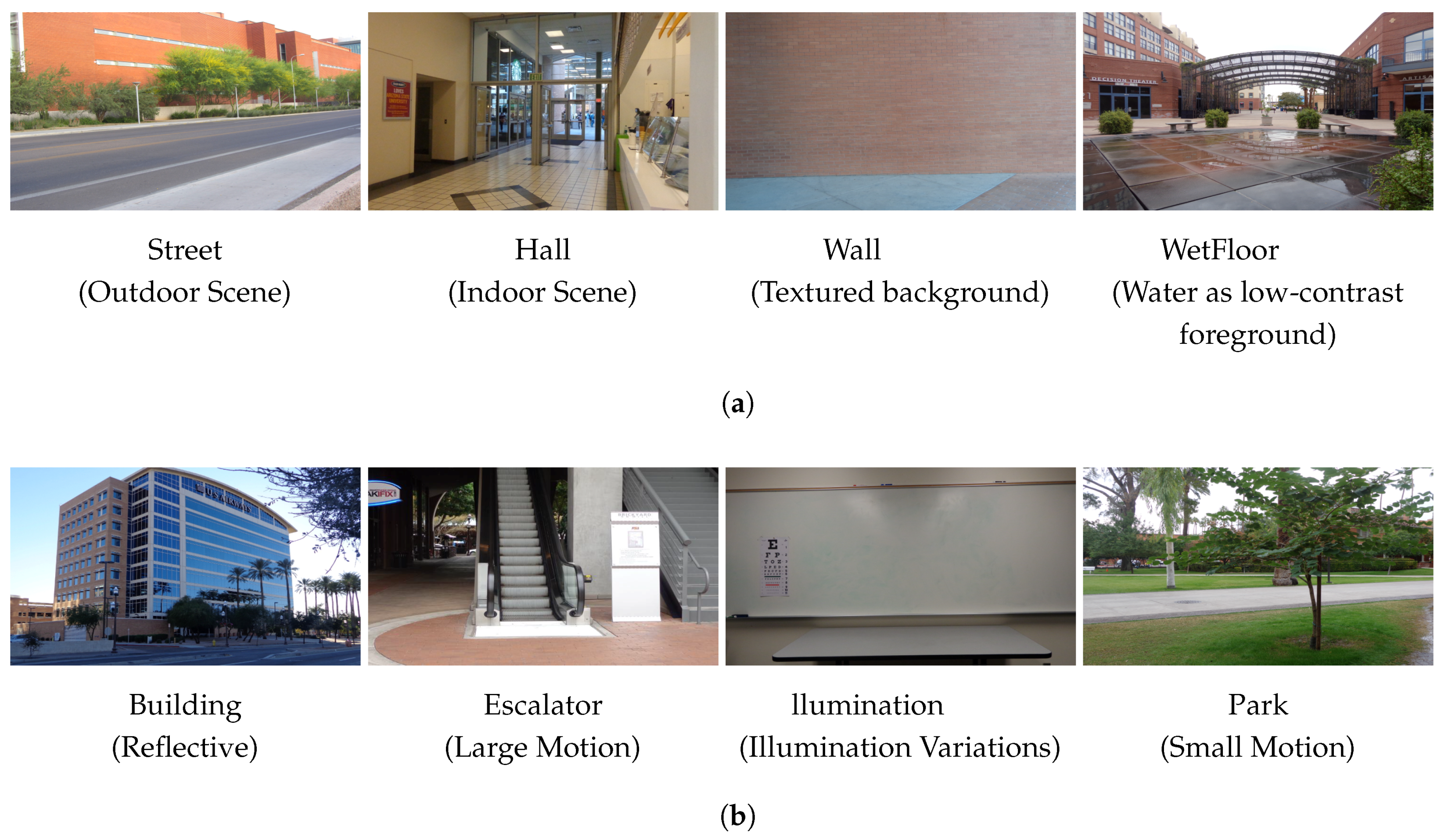
3.1. Datasets
3.1.1. Reconstructed Background Quality (ReBaQ) Dataset
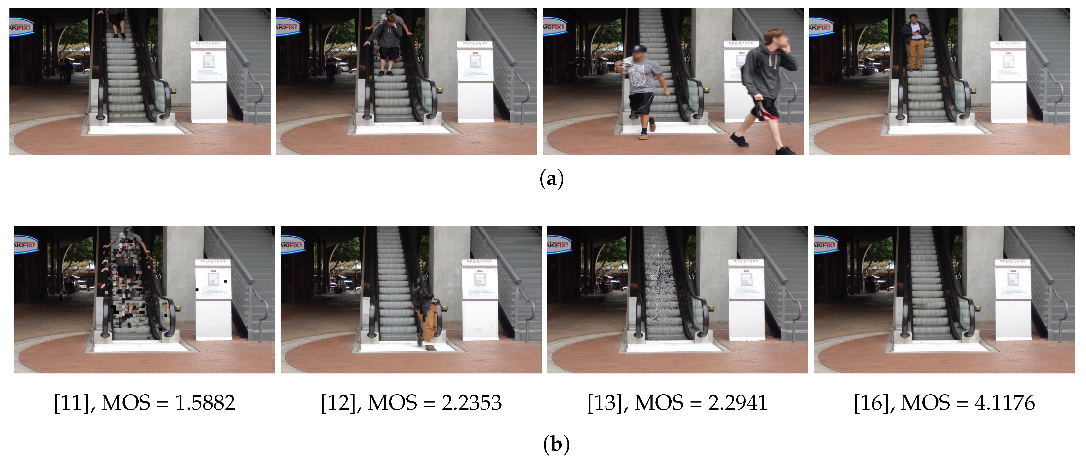
3.1.2. SBMNet Based Reconstructed Background Quality (S-ReBaQ) Dataset
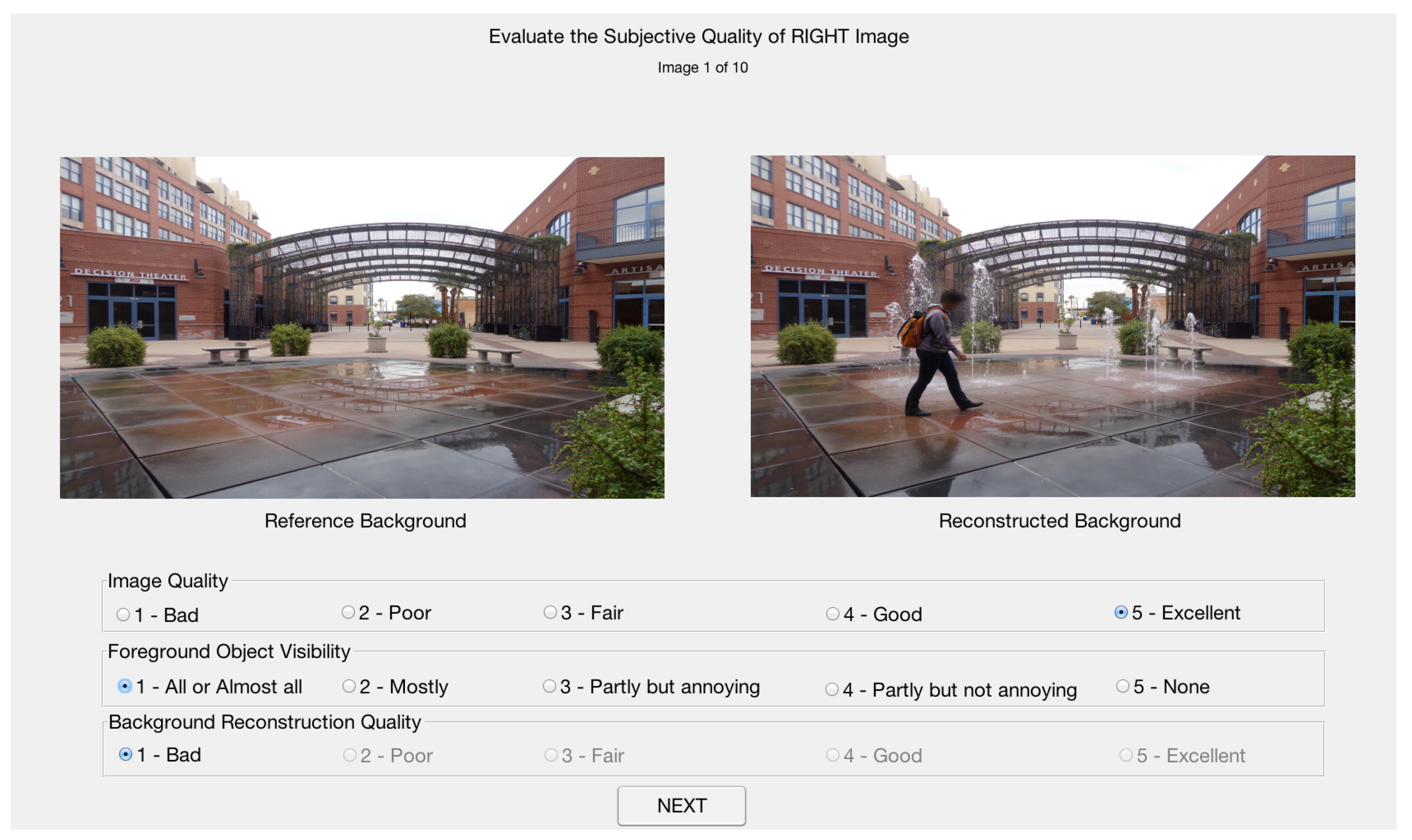
3.2. Subjective Evaluation
4. Proposed Reconstructed Background Quality Index
- (i)
- the visibility of the foreground objects, and
- (ii)
- the visible artifacts introduced while reconstructing the background image.
4.1. Structure Difference Map ()
4.2. Color Distance ()
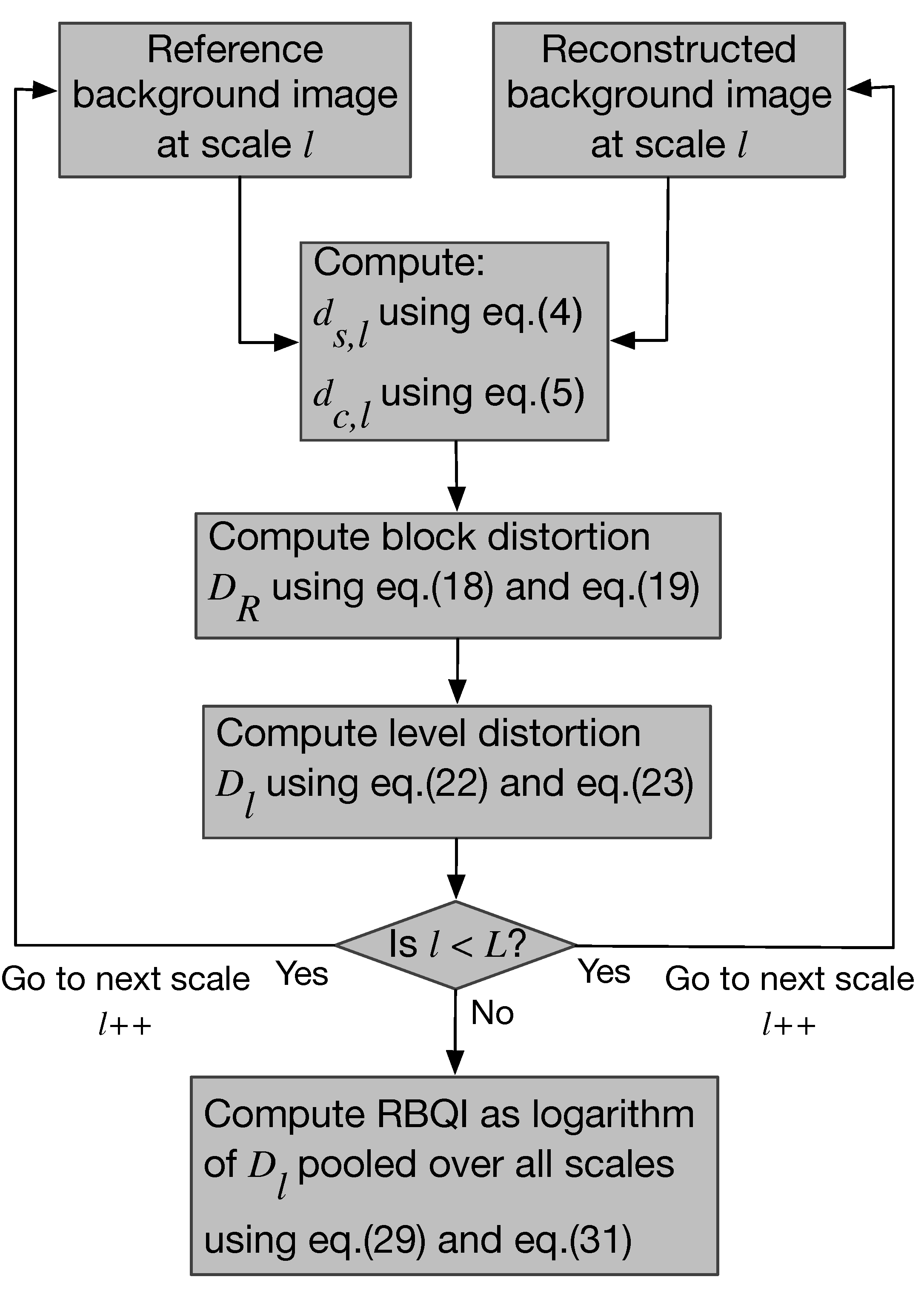
4.3. Computation of the Reconstructed Background Quality Index (RBQI) Based on Probability Summation
5. Results
5.1. Performance Comparison
5.2. Model Parameter Selection
5.3. Sensitivity Analysis
6. Conclusions
Supplementary Materials
Author Contributions
Funding
Conflicts of Interest
Abbreviations
| RBQI | Reconstructed Background Quality Index |
| PSNR | Peak Signal to Noise Ratio |
| AGE | Average Gray-level Error |
| EPs | Number of Error Pixels |
| pEPs | percentage of Error Pixels |
| CEPs | number of Clustered Error Pixels |
| pCEPs | percentage of Clustered Error Pixels |
| IQA | Image Quality Analysis |
| FR-IQA | Full Reference Image Quality Assessment |
| HVS | Human Visual System |
| MS-SSIM | Multi-scale Structural SIMilarity index |
| CQM | Color image Quality Measures |
| PETS | Performance Evaluation of Tracking and Surveillance |
| SBMNet | Scene Background Modeling Net |
| SSIM | Structural SIMilarity index |
| VSNR | Visual Signal to Noise ratio |
| VIF | Visual Information Fidelity |
| VIFP | pixel-based Visual Information Fidelity |
| UQI | Universal Quality Index |
| IFC | Image Fidelity Criterion |
| NQM | Noise Quality Measure |
| WSNR | Weights Signal to Noise Ratio |
| FSIM | Feature SIMilarity index |
| FSIMc | Feature SIMilarity index with color |
| SR-SIM | Spectral Residual SIMilarity index |
| SalSSIM | Saliency-based Structural SIMilarity index |
| ReBaQ | Reconstructed Background Quality dataset |
| S-ReBaQ | SBMNet based Reconstructed Background Quality dataset |
| SBMC | Scene Background Modeling |
| MOS | Mean Opinion Score |
| PCC | Pearson Correlation Coefficient |
| SROCC | Spearman Rank Order Correlation Coefficient |
| RMSE | Root Mean Square Error |
| OR | Outlier Ratio |
References
- Colque, R.M.; Cámara-Chávez, G. Progressive Background Image Generation of Surveillance Traffic Videos Based on a Temporal Histogram Ruled by a Reward/Penalty Function. In Proceedings of the 2011 24th SIBGRAPI Conference on Graphics, Patterns and Images (Sibgrapi), Maceio, Brazil, 28–31 August 2011; pp. 297–304. [Google Scholar]
- Stauffer, C.; Grimson, W.E.L. Learning patterns of activity using real-time tracking. IEEE Trans. Pattern Anal. Mach. Intell. 2000, 22, 747–757. [Google Scholar] [CrossRef]
- Li, L.; Huang, W.; Gu, I.Y.H.; Tian, Q. Statistical modeling of complex backgrounds for foreground object detection. IEEE Trans. Image Process. 2004, 13, 1459–1472. [Google Scholar] [CrossRef] [PubMed]
- Fleuret, F.; Berclaz, J.; Lengagne, R.; Fua, P. Multicamera People Tracking with a Probabilistic Occupancy Map. IEEE Trans. Pattern Anal. Mach. Intell. 2008, 30, 267–282. [Google Scholar] [CrossRef] [PubMed]
- Flores, A.; Belongie, S. Removing pedestrians from google street view images. In Proceedings of the IEEE Computer Society Conference on Computer Vision and Pattern Recognition Workshops, San Francisco, CA, USA, 13–18 June 2010; pp. 53–58. [Google Scholar]
- Jones, W.D. Microsoft and Google vie for virtual world domination. IEEE Spectr. 2006, 43, 16–18. [Google Scholar] [CrossRef]
- Zheng, E.; Chen, Q.; Yang, X.; Liu, Y. Robust 3D modeling from silhouette cues. In Proceedings of the IEEE International Conference on Acoustics, Speech and Signal Processing, Taipei, Taiwan, 19–24 April 2009; pp. 1265–1268. [Google Scholar]
- Maddalena, L.; Petrosino, A. A Self-Organizing Approach to Background Subtraction for Visual Surveillance Applications. IEEE Trans. Image Process. 2008, 17, 1168–1177. [Google Scholar] [CrossRef] [PubMed]
- Varadarajan, S.; Karam, L.; Florencio, D. Background subtraction using spatio-temporal continuities. In Proceedings of the 2010 2nd European Workshop on Visual Information Processing, Paris, France, 5–6 July 2010; pp. 144–148. [Google Scholar]
- Farin, D.; de With, P.; Effelsberg, W. Robust background estimation for complex video sequences. In Proceedings of the IEEE International Conference on Image Processing, Barcelona, Spain, 14–17 September 2003; Volume 1, pp. 145–148. [Google Scholar]
- Hsiao, H.H.; Leou, J.J. Background initialization and foreground segmentation for bootstrapping video sequences. EURASIP J. Image Video Process. 2013, 1, 12. [Google Scholar] [CrossRef]
- Reddy, V.; Sanderson, C.; Lovell, B. A low-complexity algorithm for static background estimation from cluttered image sequences in surveillance contexts. EURASIP J. Image Video Process. 2010, 1, 1:1–1:14. [Google Scholar] [CrossRef]
- Yao, J.; Odobez, J. Multi-Layer Background Subtraction Based on Color and Texture. In Proceedings of the IEEE Conference on Computer Vision and Pattern Recognition, Minneapolis, MN, USA, 17–22 June 2007; pp. 1–8. [Google Scholar]
- Colombari, A.; Fusiello, A. Patch-Based Background Initialization in Heavily Cluttered Video. IEEE Trans. Image Process. 2010, 19, 926–933. [Google Scholar] [CrossRef] [PubMed]
- Herley, C. Automatic occlusion removal from minimum number of images. In Proceedings of the IEEE International Conference on Image Processing, Genova, Italy, 14 September 2005; Volume 2, pp. 1046–1049. [Google Scholar]
- Agarwala, A.; Dontcheva, M.; Agrawala, M.; Drucker, S.; Colburn, A.; Curless, B.; Salesin, D.; Cohen, M. Interactive Digital Photomontage. ACM Trans. Gr. 2004, 23, 294–302. [Google Scholar] [CrossRef]
- Shrotre, A.; Karam, L. Background recovery from multiple images. In Proceedings of the IEEE Digital Signal Processing and Signal Processing Education Meeting, Napa, CA, USA, 11–14 August 2013; pp. 135–140. [Google Scholar]
- Maddalena, L.; Petrosino, A. Towards Benchmarking Scene Background Initialization. In 2015 ICIAP: New Trends in Image Analysis and Processing—ICIAP 2015 Workshops; Springer: Berlin, Germany, 2015; pp. 469–476. [Google Scholar]
- Wang, Z.; Simoncelli, E.; Bovik, A. Multiscale structural similarity for image quality assessment. In Proceedings of the Asilomar Conference on Signals, Systems and Computers, Pacific Grove, CA, USA, 9–12 November 2003; Volume 2, pp. 1398–1402. [Google Scholar]
- Yalman, Y.; Ertürk, İ. A new color image quality measure based on YUV transformation and PSNR for human vision system. Turk. J. Electr. Eng. Comput. Sci. 2013, 21, 603–612. [Google Scholar]
- Bouwmans, T.; Maddalena, L.; Petrosino, A. Scene background initialization: A taxonomy. Pattern Recognit. Lett. 2017, 96, 3–11. [Google Scholar] [CrossRef]
- Maddalena, L.; Jodoin, P. Scene Background Modeling Contest (SBMC2016). Available online: http://www.icpr2016.org/site/session/scene-background-modeling-sbmc2016/ (accessed on 15 May 2018).
- Toyama, K.; Krumm, J.; Brumitt, B.; Meyers, B. Wallflower: principles and practice of background maintenance. In Proceedings of the IEEE International Conference on Computer Vision, Kerkyra, Greece, 20–27 September 1999; Volume 1, pp. 255–261. [Google Scholar]
- Mahadevan, V.; Vasconcelos, N. Spatiotemporal Saliency in Dynamic Scenes. IEEE Trans. Pattern Anal. Mach. Intell. 2010, 32, 171–177. [Google Scholar] [CrossRef] [PubMed]
- Sheikh, Y.; Shah, M. Bayesian modeling of dynamic scenes for object detection. IEEE Trans. Pattern Anal. Mach. Intell. 2005, 27, 1778–1792. [Google Scholar] [CrossRef] [PubMed]
- Jodoin, P.; Maddalena, L.; Petrosino, A. SceneBackgroundModeling.Net (SBMnet). Available online: www.SceneBackgroundModeling.net (accessed on 15 May 2018).
- Jodoin, P.M.; Maddalena, L.; Petrosino, A.; Wang, Y. Extensive Benchmark and Survey of Modeling Methods for Scene Background Initialization. IEEE Trans. Image Process. 2017, 26, 5244–5256. [Google Scholar] [CrossRef] [PubMed]
- Shrotre, A.; Karam, L. Visual quality assessment of reconstructed background images. In Proceedings of the International Conference on Quality of Multimedia Experience, Lisbon, Portugal, 6–8 June 2016; pp. 1–6. [Google Scholar]
- Wang, Z.; Bovik, A.; Sheikh, H.; Simoncelli, E. Image quality assessment: From error visibility to structural similarity. IEEE Trans. Image Process. 2004, 13, 600–612. [Google Scholar] [CrossRef] [PubMed]
- Chandler, D.; Hemami, S. VSNR: A Wavelet-Based Visual Signal to Noise Ratio for Natural Images. IEEE Trans. Image Process. 2007, 16, 2284–2298. [Google Scholar] [CrossRef] [PubMed]
- Sheikh, H.; Bovik, A. Image information and visual quality. IEEE Trans. Image Process. 2006, 15, 430–444. [Google Scholar] [CrossRef] [PubMed]
- Wang, Z.; Bovik, A. A universal image quality index. IEEE Sign. Process. Lett. 2002, 9, 81–84. [Google Scholar] [CrossRef]
- Sheikh, H.; Bovik, A.; de Veciana, G. An information fidelity criterion for image quality assessment using natural scene statistics. IEEE Trans. Image Process. 2005, 14, 2117–2128. [Google Scholar] [CrossRef] [PubMed]
- Damera-Venkata, N.; Kite, T.; Geisler, W.; Evans, B.; Bovik, A. Image quality assessment based on a degradation model. IEEE Trans. Image Process. 2000, 9, 636–650. [Google Scholar] [CrossRef] [PubMed]
- Mitsa, T.; Varkur, K. Evaluation of contrast sensitivity functions for the formulation of quality measures incorporated in halftoning algorithms. In Proceedings of the IEEE International Conference on Acoustics Speech, and Signal Processing, Minneapolis, MN, USA, 27–30 April 1993; Volume 5, pp. 301–304. [Google Scholar]
- Zhang, L.; Zhang, D.; Mo, X.; Zhang, D. FSIM: A Feature Similarity Index for Image Quality Assessment. IEEE Trans. Image Process. 2011, 20, 2378–2386. [Google Scholar] [CrossRef] [PubMed]
- Zhang, L.; Li, H. SR-SIM: A fast and high performance IQA index based on spectral residual. In Proceedings of the 2012 19th IEEE International Conference on Image Processing, Orlando, FL, USA, 30 September–3 October 2012; pp. 1473–1476. [Google Scholar]
- Akamine, W.; Farias, M. Incorporating visual attention models into video quality metrics. In Proceedings of SPIE; SPIE: Bellingham, WA, USA, 2014; Volume 9016, pp. 1–9. [Google Scholar]
- Lin, W.; Kuo, J.C.C. Perceptual visual quality metrics: A survey. J. Vis. Commun. Image Represent. 2011, 22, 297–312. [Google Scholar] [CrossRef]
- Chandler, D.M. Seven Challenges in Image Quality Assessment: Past, Present, and Future Research. ISRN Signal Process. 2013, 1–53. [Google Scholar] [CrossRef]
- Seshadrinathan, K.; Pappas, T.N.; Safranek, R.J.; Chen, J.; Wang, Z.; Sheikh, H.R.; Bovik, A.C. Image Quality Assessment. In The Essential Guide to Image Processing; Bovik, A.C., Ed.; Elsevier: New York, NY, USA, 2009; Chapter 21; pp. 553–595. [Google Scholar]
- Laugraud, B.; Piérard, S.; Van Droogenbroeck, M. LaBGen-P: A pixel-level stationary background generation method based on LaBGen. In Proceedings of the 2016 23rd International Conference on Pattern Recognition, Cancun, Mexico, 4–8 December 2016; pp. 107–113. [Google Scholar]
- Maddalena, L.; Petrosino, A. Extracting a background image by a multi-modal scene background model. In Proceedings of the 2016 23rd International Conference on Pattern Recognition, Cancun, Mexico, 4–8 December 2016; pp. 143–148. [Google Scholar]
- Javed, S.; Jung, S.K.; Mahmood, A.; Bouwmans, T. Motion-Aware Graph Regularized RPCA for background modeling of complex scenes. In Proceedings of the 2016 23rd International Conference on Pattern Recognition, Cancun, Mexico, 4–8 December 2016; pp. 120–125. [Google Scholar]
- Liu, W.; Cai, Y.; Zhang, M.; Li, H.; Gu, H. Scene background estimation based on temporal median filter with Gaussian filtering. In Proceedings of the 2016 23rd International Conference on Pattern Recognition, Cancun, Mexico, 4–8 December 2016; pp. 132–136. [Google Scholar]
- Ramirez-Alonso, G.; Ramirez-Quintana, J.A.; Chacon-Murguia, M.I. Temporal weighted learning model for background estimation with an automatic re-initialization stage and adaptive parameters update. Pattern Recognit. Lett. 2017, 96, 34–44. [Google Scholar] [CrossRef]
- Minematsu, T.; Shimada, A.; Taniguchi, R.I. Background initialization based on bidirectional analysis and consensus voting. In Proceedings of the 2016 23rd International Conference on Pattern Recognition, Cancun, Mexico, 4–8 December 2016; pp. 126–131. [Google Scholar]
- Piccardi, M. Background subtraction techniques: A review. In Proceedings of the IEEE International Conference on Systems, Man and Cybernetics, The Hague, The Netherlands, 10–13 October 2004; Volume 4, pp. 3099–3104. [Google Scholar]
- Halfaoui, I.; Bouzaraa, F.; Urfalioglu, O. CNN-based initial background estimation. In Proceedings of the 2016 23rd International Conference on Pattern Recognition, Cancun, Mexico, 4–8 December 2016; pp. 101–106. [Google Scholar]
- Chacon-Murguia, M.I.; Ramirez-Quintana, J.A.; Ramirez-Alonso, G. Evaluation of the background modeling method Auto-Adaptive Parallel Neural Network Architecture in the SBMnet dataset. In Proceedings of the 2016 23rd International Conference on Pattern Recognition, Cancun, Mexico, 4–8 December 2016; pp. 137–142. [Google Scholar]
- Ortego, D.; SanMiguel, J.C.; Martínez, J.M. Rejection based multipath reconstruction for background estimation in SBMnet 2016 dataset. In Proceedings of the 2016 23rd International Conference on Pattern Recognition, Cancun, Mexico, 4–8 December 2016; pp. 114–119. [Google Scholar]
- Methodology for the Subjective Assessment of the Quality of Television Pictures; Technical Report ITU-R BT.500-13; International Telecommunications Union: Geneva, Switzerland, 2012.
- Snellen, H. Probebuchstaben zur Bestimmung der Sehschärfe; P.W. Van de Weijer: Utrecht, The Netherlands, 1862. [Google Scholar]
- Waggoner, T.L. PseudoIsochromatic Plate (PIP) Color Vision Test 24 Plate Edition. Available online: http://colorvisiontesting.com/ishihara.htm (accessed on 15 May 2018).
- Robson, J.; Graham, N. Probability summation and regional variation in contrast sensitivity across the visual field. Vis. Res. 1981, 21, 409–418. [Google Scholar] [CrossRef]
- Su, J.; Mersereau, R. Post-procesing for artifact reduction in JPEG-compressed images. In Proceedings of the IEEE International Conference on Acoustics, Speech, and Signal Processing, Detroit, MI, USA, 9–12 May 1995; pp. 2363–2366. [Google Scholar]
- Chou, C.H.; Liu, K.C. Colour image compression based on the measure of just noticeable colour difference. IET Image Process. 2008, 2, 304–322. [Google Scholar] [CrossRef]
- Mahy, M.; Eycken, L.; Oosterlinck, A. Evaluation of uniform color spaces developed after the adoption of CIELAB and CIELUV. Color Res. Appl. 1994, 19, 105–121. [Google Scholar]
- Watson, A.; Kreslake, L. Measurement of visual impairment scales for digital video. In Human Vision and Electronic Imaging VI; International Society for Optics and Photonics: Bellingham, WA, USA, 2001; Volume 4299, pp. 79–89. [Google Scholar]
- Watson, A.B. DCT quantization matrices visually optimized for individual images. In Human Vision and Electronic Imaging VI; International Society for Optics and Photonics: Bellingham, WA, USA, 1993; Volume 1913, pp. 202–216. [Google Scholar]
- Hontsch, I.; Karam, L.J. Adaptive image coding with perceptual distortion control. IEEE Trans. Image Process. 2002, 11, 213–222. [Google Scholar] [CrossRef] [PubMed]
- VQEG. Final Report from the Video Quality Experts Group on the Validation of Objective Models of Video Quality Assessment. 2003. Available online: ftp://vqeg.its.bldrdoc.gov/Documents/VQEGApprovedFinalReports/VQEGIIFinalReport.pdf (accessed on 15 May 2018).
- Mittal, A.; Moorthy, A.; Bovik, A. No-Reference Image Quality Assessment in the Spatial Domain. IEEE Trans. Image Process. 2012, 21, 4695–4708. [Google Scholar] [CrossRef] [PubMed]


| a. Comparison on the ReBaQ-Static Dataset. | |||||||
| ReBaQ-Static | |||||||
| PCC | SROCC | RMSE | OR | PPCC | PSROCC | ||
| Statistical Measures | AGE | 0.7776 | 0.6348 | 0.6050 | 9.72% | 0.000000 | 0.000000 |
| EPs | 0.3976 | 0.5093 | 0.8829 | 13.89% | 0.000000 | 0.000000 | |
| pEPs | 0.8058 | 0.6170 | 0.5698 | 6.94% | 0.000000 | 0.000000 | |
| CEPs | 0.5719 | 0.6939 | 0.7893 | 11.11% | 0.000000 | 0.000000 | |
| pCEPs | 0.6281 | 0.7843 | 0.9622 | 13.89% | 0.000000 | 0.000000 | |
| Image Quality Assessment Metrics | PSNR | 0.8324 | 0.7040 | 0.5331 | 8.33% | 0.000000 | 0.000000 |
| SSIM [29] | 0.5914 | 0.5168 | 0.7759 | 11.11% | 0.000000 | 0.000177 | |
| MS-SSIM [19] | 0.7230 | 0.7085 | 0.6648 | 8.33% | 0.000000 | 0.000000 | |
| VSNR [30] | 0.5216 | 0.3986 | 0.8209 | 9.72% | 0.000003 | 0.000531 | |
| VIF [31] | 0.3625 | 0.0843 | 0.8968 | 15.28% | 0.001754 | 0.484429 | |
| VIFP [31] | 0.5122 | 0.3684 | 0.8265 | 11.11% | 0.000004 | 0.001470 | |
| UQI [32] | 0.6197 | 0.7581 | 0.9622 | 13.89% | 0.000000 | 0.000000 | |
| IFC [33] | 0.5003 | 0.3771 | 0.8331 | 11.11% | 0.000008 | 0.001105 | |
| NQM [34] | 0.8251 | 0.8602 | 0.5437 | 6.94% | 0.000000 | 0.000000 | |
| WSNR [35] | 0.8013 | 0.7389 | 0.5756 | 5.56% | 0.000000 | 0.000000 | |
| FSIM [36] | 0.7209 | 0.6970 | 0.6668 | 9.72% | 0.000000 | 0.000000 | |
| FSIMc [36] | 0.7274 | 0.7033 | 0.6603 | 9.72% | 0.000000 | 0.000000 | |
| SRSIM [37] | 0.7906 | 0.7862 | 0.5892 | 8.33% | 0.000000 | 0.000000 | |
| SalSSIM [38] | 0.5983 | 0.5217 | 0.7710 | 9.72% | 0.000000 | 0.000003 | |
| CQM [20] | 0.6401 | 0.5755 | 0.7393 | 8.33% | 0.000000 | 0.000000 | |
| RBQI(Proposed) | 0.9006 | 0.8592 | 0.4183 | 4.17% | 0.000000 | 0.000000 | |
| b. Comparison on the ReBaQ-Dynamic Dataset. | |||||||
| ReBaQ-Dynamic | |||||||
| PCC | SROCC | RMSE | OR | PPCC | PSROCC | ||
| Statistical Measures | AGE | 0.4999 | 0.2303 | 0.7644 | 9.72% | 0.005000 | 0.051600 |
| EPs | 0.1208 | 0.2771 | 0.8761 | 13.89% | 0.007600 | 0.018500 | |
| pEPs | 0.4734 | 0.2771 | 0.8825 | 9.72% | 0.007600 | 0.018500 | |
| CEPs | 0.5951 | 0.7549 | 0.7092 | 11.11% | 0.000000 | 0.000000 | |
| pCEPs | 0.6418 | 0.7940 | 0.8826 | 15.28% | 0.000000 | 0.000000 | |
| Image Quality Assessment Metrics | PSNR | 0.5133 | 0.4179 | 0.7575 | 8.33% | 0.000004 | 0.000263 |
| SSIM [29] | 0.0135 | 0.0264 | 0.8826 | 15.28% | 0.910238 | 0.822439 | |
| MS-SSIM [19] | 0.5087 | 0.4466 | 0.7598 | 9.72% | 0.000005 | 0.000085 | |
| VSNR [30] | 0.5090 | 0.1538 | 0.7597 | 9.72% | 0.000005 | 0.198310 | |
| VIF [31] | 0.3103 | 0.3328 | 0.8390 | 13.89% | 0.199921 | 0.236522 | |
| VIFP [31] | 0.4864 | 0.1004 | 0.7711 | 9.72% | 0.000015 | 0.403684 | |
| UQI [32] | 0.6262 | 0.7450 | 0.8826 | 15.28% | 0.000000 | 0.000000 | |
| IFC [33] | 0.4306 | 0.1024 | 0.7966 | 11.11% | 0.000160 | 0.394409 | |
| NQM [34] | 0.6898 | 0.6600 | 0.6390 | 9.72% | 0.000000 | 0.000000 | |
| WSNR [35] | 0.6409 | 0.5760 | 0.6775 | 9.72% | 0.000000 | 0.000000 | |
| FSIM [36] | 0.5131 | 0.3283 | 0.7575 | 9.72% | 0.000004 | 0.004922 | |
| FSIMc [36] | 0.5144 | 0.3310 | 0.7568 | 9.72% | 0.000004 | 0.004559 | |
| SRSIM [37] | 0.5512 | 0.5376 | 0.7364 | 11.11% | 0.000001 | 0.000001 | |
| SalSSIM [38] | 0.4866 | 0.3200 | 0.7710 | 9.72% | 0.000015 | 0.006198 | |
| CQM [20] | 0.7050 | 0.7610 | 0.6259 | 8.33% | 0.000000 | 0.000000 | |
| RBQI(Proposed) | 0.7908 | 0.6773 | 0.5402 | 5.56% | 0.000000 | 0.000000 | |
| S-ReBaQ | |||||||
|---|---|---|---|---|---|---|---|
| PCC | SROCC | RMSE | OR | PPCC | PSROCC | ||
| Statistical Measures | AGE | 0.6453 | 0.6238 | 2.2373 | 14.84% | 0.392900 | 0.000000 |
| EPs | 0.4202 | 0.1426 | 1.2049 | 24.73% | 0.000000 | 0.000000 | |
| pEPs | 0.0505 | 0.4990 | 1.6676 | 26.92% | 0.498331 | 0.000000 | |
| CEPs | 0.6283 | 0.6666 | 0.8491 | 18.68% | 0.000000 | 0.000000 | |
| pCEPs | 0.8346 | 0.8380 | 0.6011 | 6.59% | 0.000000 | 0.000000 | |
| Image Quality Assessment Metrics | PSNR | 0.7099 | 0.6834 | 0.7686 | 6.59% | 0.000000 | 0.000000 |
| SSIM [29] | 0.5975 | 0.5827 | 0.8751 | 12.09% | 0.000000 | 0.000000 | |
| MS-SSIM [19] | 0.8048 | 0.8030 | 0.6478 | 29.12% | 0.000000 | 0.000000 | |
| VSNR [30] | 0.0850 | 0.1717 | 1.0874 | 13.19% | 0.253675 | 0.486686 | |
| VIF [31] | 0.1027 | 0.2064 | 1.0914 | 27.47% | 0.167842 | 0.005305 | |
| VIFP [31] | 0.6081 | 0.6240 | 0.8664 | 26.92% | 0.000000 | 0.000000 | |
| UQI [32] | 0.6316 | 0.5932 | 0.8461 | 14.84% | 0.000000 | 0.000000 | |
| IFC [33] | 0.6235 | 0.6020 | 0.8533 | 16.48% | 0.000000 | 0.000000 | |
| NQM [34] | 0.7950 | 0.7816 | 0.6621 | 14.84% | 0.000000 | 0.000000 | |
| WSNR [35] | 0.7176 | 0.6888 | 0.7601 | 7.14% | 0.000000 | 0.000000 | |
| FSIM [36] | 0.7243 | 0.7157 | 0.7525 | 10.44% | 0.000000 | 0.000000 | |
| FSIMc [36] | 0.7278 | 0.7172 | 0.7484 | 12.09% | 0.000000 | 0.000000 | |
| SRSIM [37] | 0.7853 | 0.7538 | 0.6757 | 12.09% | 0.000000 | 0.000000 | |
| SalSSIM [38] | 0.7356 | 0.7300 | 0.7393 | 7.14% | 0.000000 | 0.000000 | |
| CQM [20] | 0.2634 | 0.3645 | 1.0531 | 8.24% | 0.000327 | 0.000276 | |
| RBQI(Proposed) | 0.8613 | 0.8222 | 0.5545 | 3.30% | 0.000000 | 0.000000 | |
| ReBaQ and S-ReBaQ Combined | |||||||
|---|---|---|---|---|---|---|---|
| PCC | SROCC | RMSE | OR | PPCC | PSROCC | ||
| Statistical Measures | AGE | 0.6667 | 0.6593 | 0.8462 | 14.42% | 0.000000 | 0.000000 |
| EPs | 0.5744 | 0.6353 | 0.9294 | 19.02% | 0.000000 | 0.000000 | |
| pEPs | 0.1456 | 0.6939 | 1.1233 | 29.45% | 0.008464 | 0.000000 | |
| CEPs | 0.6202 | 0.6967 | 0.8906 | 18.40% | 0.000000 | 0.000000 | |
| pCEPs | 0.8427 | 0.8421 | 0.6113 | 7.06% | 0.000000 | 0.000000 | |
| Image Quality Assessment Metrics | PSNR | 0.7306 | 0.7166 | 0.7753 | 10.74% | 0.000000 | 0.000000 |
| SSIM [29] | 0.6083 | 0.5743 | 0.9011 | 16.56% | 0.000000 | 0.000000 | |
| MS-SSIM [19] | 0.7874 | 0.7907 | 0.6999 | 8.59% | 0.000000 | 0.000000 | |
| VSNR [30] | 0.1789 | 0.3459 | 1.1171 | 29.75% | 0.001176 | 0.001126 | |
| VIF [31] | 0.3478 | 0.5601 | 1.0645 | 25.77% | 0.000000 | 0.000000 | |
| VIFP [31] | 0.6281 | 0.5911 | 0.8835 | 14.72% | 0.000000 | 0.000000 | |
| UQI [32] | 0.7024 | 0.6778 | 0.8081 | 12.27% | 0.000000 | 0.000000 | |
| IFC [33] | 0.6455 | 0.5976 | 0.8671 | 14.42% | 0.00000 | 0.000000 | |
| NQM [34] | 0.7800 | 0.7781 | 0.7106 | 9.51% | 0.000000 | 0.000000 | |
| WSNR [35] | 0.7669 | 0.7550 | 0.7286 | 10.74% | 0.000000 | 0.000000 | |
| FSIM [36] | 0.7294 | 0.7088 | 0.7767 | 11.35% | 0.000000 | 0.000000 | |
| FSIMc [36] | 0.7337 | 0.7117 | 0.7715 | 11.35% | 0.000000 | 0.000000 | |
| SRSIM [37] | 0.7842 | 0.7875 | 0.7045 | 8.90% | 0.000000 | 0.000000 | |
| SalSSIM [38] | 0.7157 | 0.6960 | 0.7930 | 11.35% | 0.000000 | 0.000000 | |
| CQM [20] | 0.5651 | 0.5429 | 0.9367 | 21.78% | 0.000000 | 0.000000 | |
| RBQI(Proposed) | 0.8770 | 0.8372 | 0.5456 | 4.29% | 0.000000 | 0.000000 | |
| a. Simulation results with different neighborhood search window sizes nhood. | ||||||||
| ReBaQstatic | ReBaQdynamic | |||||||
| PCC | SROCC | RMSE | OR | PCC | SROCC | RMSE | OR | |
| nhood = 1 | 0.7931 | 0.8314 | 0.5077 | 12.50% | 0.6395 | 0.6539 | 0.5662 | 11.11% |
| nhood = 9 | 0.9015 | 0.8581 | 0.4911 | 6.94% | 0.7834 | 0.6683 | 0.5394 | 6.94% |
| nhood = 17 | 0.9006 | 0.8581 | 0.4837 | 4.17% | 0.7908 | 0.6762 | 0.4374 | 5.56% |
| nhood = 33 | 0.9001 | 0.8581 | 0.4896 | 5.56% | 0.7818 | 0.6683 | 0.4769 | 5.56% |
| b. Simulation results with different number of scales L | ||||||||
| ReBaQstatic | ReBaQdynamic | |||||||
| PCC | SROCC | RMSE | OR | PCC | SROCC | RMSE | OR | |
| L = 1 | 0.8190 | 0.8183 | 0.6667 | 8.33% | 0.5561 | 0.5520 | 0.7335 | 12.50% |
| L = 2 | 0.8597 | 0.8310 | 0.5521 | 5.56% | 0.7281 | 0.6482 | 0.6050 | 5.56% |
| L = 3 | 0.9006 | 0.8592 | 0.5077 | 4.17% | 0.7908 | 0.6773 | 0.5662 | 5.56% |
| L = 4 | 0.9006 | 0.8581 | 0.4915 | 4.17% | 0.7954 | 0.6797 | 0.5350 | 5.56% |
| L = 5 | 0.9006 | 0.8581 | 0.4883 | 5.56% | 0.8087 | 0.6881 | 0.5191 | 5.56% |
| ReBaQ-Static | ReBaQ-Dynamic | ||||||||
|---|---|---|---|---|---|---|---|---|---|
| n= 24 | n= 50 | n= 24 | n= 50 | ||||||
| Statistical Measures | AGE | 0.8154 | 0.0451 | 0.7898 | 0.0108 | 0.4824 | 0.0504 | 0.5164 | 0.0123 |
| EPs | 0.6333 | 0.1149 | 0.4834 | 0.0801 | 0.1627 | 0.0960 | 0.1499 | 0.0866 | |
| pEPs | 0.8309 | 0.0452 | 0.8147 | 0.0088 | 0.4437 | 0.0573 | 0.4819 | 0.0061 | |
| CEPs | 0.6851 | 0.0941 | 0.6184 | 0.0923 | 0.7475 | 0.0488 | 0.6223 | 0.1500 | |
| pCEPs | 0.8556 | 0.0500 | 0.8178 | 0.0451 | 0.8327 | 0.0504 | 0.6644 | 0.0185 | |
| Image Quality Assessment Metrics | PSNR | 0.8620 | 0.0398 | 0.8410 | 0.0067 | 0.5113 | 0.0503 | 0.5290 | 0.0172 |
| SSIM [29] | 0.5578 | 0.0862 | 0.5775 | 0.0084 | 0.2372 | 0.2250 | 0.2290 | 0.2376 | |
| MS-SSIM [19] | 0.7729 | 0.0510 | 0.7401 | 0.0123 | 0.5253 | 0.0750 | 0.5232 | 0.0131 | |
| VSNR [30] | 0.5365 | 0.0844 | 0.5225 | 0.0182 | 0.4926 | 0.0287 | 0.5212 | 0.0101 | |
| VIF [31] | 0.0798 | 0.3740 | 0.0571 | 0.3245 | 0.2242 | 0.2474 | 0.1902 | 0.1916 | |
| VIFP [31] | 0.5453 | 0.1259 | 0.5264 | 0.0302 | 0.4515 | 0.0167 | 0.4941 | 0.0057 | |
| UQI [32] | 0.7616 | 0.0831 | 0.6658 | 0.0241 | 0.8105 | 0.0426 | 0.6545 | 0.0210 | |
| IFC [33] | 0.5249 | 0.0906 | 0.5067 | 0.0189 | 0.4346 | 0.0254 | 0.4410 | 0.0049 | |
| NQM [34] | 0.8619 | 0.0300 | 0.8427 | 0.0120 | 0.7564 | 0.0511 | 0.7127 | 0.0196 | |
| WSNR [35] | 0.8520 | 0.0392 | 0.8194 | 0.0149 | 0.7150 | 0.0727 | 0.6617 | 0.0238 | |
| FSIM [36] | 0.7749 | 0.0519 | 0.7421 | 0.0144 | 0.4828 | 0.0328 | 0.5202 | 0.0064 | |
| FSIMc [36] | 0.7810 | 0.0507 | 0.7481 | 0.0143 | 0.4840 | 0.0329 | 0.5213 | 0.0065 | |
| SRSIM [37] | 0.8387 | 0.0344 | 0.8132 | 0.0138 | 0.6240 | 0.0895 | 0.5756 | 0.0348 | |
| SalSSIM [38] | 0.5856 | 0.1313 | 0.5944 | 0.0103 | 0.4698 | 0.0627 | 0.4947 | 0.0059 | |
| CQM [20] | 0.7437 | 0.0793 | 0.6751 | 0.0373 | 0.7863 | 0.0593 | 0.7336 | 0.0267 | |
| RBQI(Proposed) | 0.9320 | 0.0194 | 0.9141 | 0.0084 | 0.8355 | 0.0241 | 0.8154 | 0.0107 | |
© 2018 by the authors. Licensee MDPI, Basel, Switzerland. This article is an open access article distributed under the terms and conditions of the Creative Commons Attribution (CC BY) license (http://creativecommons.org/licenses/by/4.0/).
Share and Cite
Shrotre, A.; Karam, L.J. Full Reference Objective Quality Assessment for Reconstructed Background Images. J. Imaging 2018, 4, 82. https://doi.org/10.3390/jimaging4060082
Shrotre A, Karam LJ. Full Reference Objective Quality Assessment for Reconstructed Background Images. Journal of Imaging. 2018; 4(6):82. https://doi.org/10.3390/jimaging4060082
Chicago/Turabian StyleShrotre, Aditee, and Lina J. Karam. 2018. "Full Reference Objective Quality Assessment for Reconstructed Background Images" Journal of Imaging 4, no. 6: 82. https://doi.org/10.3390/jimaging4060082
APA StyleShrotre, A., & Karam, L. J. (2018). Full Reference Objective Quality Assessment for Reconstructed Background Images. Journal of Imaging, 4(6), 82. https://doi.org/10.3390/jimaging4060082