Non-Local Sparse Image Inpainting for Document Bleed-Through Removal

Abstract

Bleed-through is a frequent, pervasive degradation in ancient manuscripts, which is caused by ink seeped from the opposite side of the sheet. Bleed-through, appearing as an extra interfering text, hinders document readability and makes it difficult to decipher the information contents. Digital image restoration techniques have been successfully employed to remove or significantly reduce this distortion. This paper proposes a two-step restoration method for documents affected by bleed-through, exploiting information from the recto and verso images. First, the bleed-through pixels are identified, based on a non-stationary, linear model of the two texts overlapped in the recto-verso pair. In the second step, a dictionary learning-based sparse image inpainting technique, with non-local patch grouping, is used to reconstruct the bleed-through-contaminated image information. An overcomplete sparse dictionary is learned from the bleed-through-free image patches, which is then used to estimate a befitting fill-in for the identified bleed-through pixels. The non-local patch similarity is employed in the sparse reconstruction of each patch, to enforce the local similarity. Thanks to the intrinsic image sparsity and non-local patch similarity, the natural texture of the background is well reproduced in the bleed-through areas, and even a possible overestimation of the bleed through pixels is effectively corrected, so that the original appearance of the document is preserved. We evaluate the performance of the proposed method on the images of a popular database of ancient documents, and the results validate the performance of the proposed method compared to the state of the art.

1. Introduction

Archival, ancient manuscripts constitute the primary carrier of most authentic information starting from the medieval era, serving as history’s own closet, carrying stories of enigmatic, unknown places or incredible events that took place in the distant past, many of which are still to be revealed. These manuscripts are of great interest and importance for historians, and provide insight into culture, civilisation, events and lifestyles of our past. With the passage of time, these documents have been exposed to different types of progressive degradations, such as spots or ink fading, due to fragile nature of the writing media, and bad storage or environmental conditions. This degradation process limits the use of these ancient classics, and some of the deteriorated documents had a very narrow escape from total annihilation. Specifically, in the manuscripts written on both sides of the sheet, often the ink had seeped through and appears as an unpleasant degradation pattern on the reverse side. Ink penetration through the paper is mainly due to aging, humidity, ink chemical properties or paper porosity [1], and can range from faint to severe. In the literature, this kind of degradation is termed as bleed-through, and impairs the legibility and interpretation of the document contents [2]. Therefore, it is of great significance to remove the bleed-through contamination and restore the integrity of the original manuscripts. An example of bleed-through removal is shown in Figure 1. Earlier, physical restoration methods were applied to deal with bleed-through degradation, but unfortunately those methods were costly, invasive, and sometimes caused permanent, irreversible damage to the documents.

In recent years, digital preservation of the documental heritage has been the focus of intensive digitisation and archiving campaigns, aimed at its distribution, accessibility and analysis. With digitization prevailing, in addition to conservation, the computing technologies applied to the digital images of these documents have quickly become a powerful and versatile tool to simplify their study and retrieval, and to facilitate new insights into the document’s contents. Digital image processing techniques can be applied to these electronic document versions, to perform any alteration to the document appearance, while preserving the original intact. Specifically, digital image processing techniques have been attempted for the virtual restoration of documents affected by bleed-through, with some impressive results. In addition, to improve the document readability, the removal of the bleed-though degradation is also a critical preprocessing step in many tasks such as feature extraction, optical character recognition, segmentation, and automatic transcription.

Bleed-through removal is a challenging task mainly due to the possible significant overlap between the original text and the bleed-through pattern, and the wide variation of its extent and intensity. In literature, bleed-through removal is addressed as a classification problem, where the document image is subdivided into three components: background (the paper support), foreground (the main text), and bleed-through [1]. Broadly speaking, the existing methods in this domain can be divided into two main categories: blind or single-sided, and non-blind or double-sided. In blind methods, the image of a single side is used, whereas the non-blind methods require the information of both the recto and verso sides of the document. Most of the earlier methods rely on the intensity information of the image and perform restoration based on the grayscale or color (red, green, blue) intensity distributions. The intensity based methods involve thresholding [3]; however, intensity information alone is insufficient as there is often a significant overlap between the foreground and bleed-through intensity profiles [4]. In addition, thresholding may also destroy other useful document features, such as stamps, annotations, or paper watermarks. Thus, intensity based thresholding is not suitable when the aim is to preserve the original appearance of the document. To overcome these drawbacks, some methods incorporate spatial information by exploiting the neighbouring structure.

Among the blind methods, in [5], an independent component analysis (ICA) method is proposed to separate the foreground, background, and bleed-through layers from an RGB image. A dual-layer Markov random field (MRF) is suggested in [6], whereas, in [7], a conditional random field (CRF) method is proposed. A multichannel based blind bleed-through removal is suggested in [8] using color decorrelation or color space transformations, whereas, in [9], a recursive unsupervised segmentation approach is applied to the data space first decorrelated by principal component analysis (PCA). In [10], bleed-through removal is addressed as a blind source separation problem, solved by using a Markov random field (MRF) based local smoothness model. Similarly, an expected maximization (EM)-based approach is suggested in [11].

As per the non-blind methods, a model based approach using differences in the intensities of recto and verso side is outlined in [12]. The same model is extended in [13] using variational models with spatial smoothness in the wavelet domain. A non-blind ICA method is outlined in [14]. Other methods of this category are proposed in [15,16,17]. The performance of the non-blind methods depends on the accurate registration of recto and verso sides of the document, which is a non-trivial pre-processing step.

For a plausible restoration of documents with bleed-through, in addition to bleed-through identification, finding a suitable replacement for the affected pixels is also essential. The restored image generated in most of the above methods is either binary, pseudo-binary (uniform background and varying foreground intensities), or textured (the bleed-through regions are replaced with an estimate of the local mean background intensity or with a random pattern). An estimate of the local mean background is used in [6,18], but such methods are good for manuscripts with a reasonably smooth background while producing visible artifacts for documents with a highly textured background. In [7], a random-fill inpainting method is suggested to replace the bleed-through pixels with background pixels randomly selected from the neighbourhood. However, the random pixel selection produces salt and pepper like artifacts in regions with large bleed-through. In [6,16], as a preliminary step, a “clean” background for the entire image is estimated, but this is usually a very laborious task. In bleed-through removal, the desired restored image is the one where the foreground and background texture is preserved as much as possible. Instead, most of the bleed-through removal methods usually concentrate on foreground text preservation, neglecting the background texture. In order to enhance the quality of the restored image, the identification of bleed-through pixels and the estimation of a tenable replacement for them should be addressed with equal attention.

Image inpainting, which refers to filling in missing or corrupted regions in an image, is a well studied and challenging topic in computer vision and image processing [19,20]. In image inpainting, the goal is to find an estimate for those regions in order to reconstruct a visually pleasant and consistent image [21]. Recently, sparse representation based image inpainting methods are reported with exquisite results [22,23]. These methods find a sparse linear combination for each image patch using an overcomplete dictionary, and then estimate the value of missing pixels in the patch. This linear sparse representation is computed adaptively, by using a earned dictionary and sparse coefficients, trained on the image at hand. A dictionary learning based method has been used for document image resolution enhancement [24], denoising [25], and restoration [26]. In addition to sparsity, non-local self-similarity is another significant property of natural images [27,28]. A number of non-local regularization terms, exploiting the non-local self-similarity, are employed in solving inverse problems [29,30]. Fusing image sparsity with non-local self-similarity produces better results in recently reported image restoration techniques [31,32]. The underlying assumption in such methods is that similar patches share the same dictionary atoms.

In this paper, we present a two-step method to restore documents affected by bleed-through using pre-registered recto and verso images. First, the bleed-through pattern is selectively identified on both sides; then, sparse image inpainting is used to find suitable fill in for the bleed-through pixels. In general, any off-the-shelf bleed-through identification methods can be used in the first step. Here, we adopt the algorithm described in [33], which is simple and very fast. Although efficient in locating the bleed-through pattern, the method in [33] lacks a proper strategy to replace the unwanted bleed-through pixels. The simple replacement with the predominant background gray level value causes unpleasant imprints of the bleed-through pattern, visible in the restored image. An interpolation based inpainting technique for such imprints is presented in [34], but the filled-in areas are mostly smooth. Here, we use a sparse image representation based inpainting, with non-local similar patches, to find a befitting fill-in for the bleed-through pixels. This sparse inpainting step, which constitutes the main contribution of the paper, enhances the quality of the restored image and preserves well the natural paper texture and the text stroke appearance. The optimization problem of sparse patch inpainting is formulated using the non-local similar patches, to account for the neighbourhood consistency, and orthogonal matching pursuit (OMP) is used to find the sparse approximation.

The rest of this paper is organized as follows. The next section briefly introduces sparse image representation and dictionary learning. Section 3 presents the non-blind bleed-through identification method. The proposed sparse image inpainting technique is described in Section 4. In Section 5, we comment on a set of experimental results, illustrating the performance of the proposed method and its comparison with state-of-the-art methods. The concluding remarks are given in Section 6.

2. Sparse Image Representation

Recently, sparse representation emerged as a powerful tool for efficient representation and processing of high-dimensional data. In particular, sparsity based regularization has achieved great success, offering solutions that outperform classical approaches in various image and signal processing applications. Among the others, we can mention inverse problems such as denoising [35,36], reconstruction [22,37], classification [38], recognition [39,40], and compression [41,42]. The underlying assumption of methods based on sparse representation is that signals such as audio and images are naturally generated by a multivariate linear model, driven by a small number of basis or regressors. The basis set, called dictionary, is either fixed and predefined, i.e., Fourier, Wavelet, Cosine, etc., or adaptively learned from a training set [43]. While the underlying key constraint of all these methods is that the observed signal is sparse, explicitly meaning that it can be adequately represented using a small set of dictionary atoms, the particularity of those based on adaptive dictionaries is that the dictionary is also learned to find the one that best describes the observed signal.

Given a data set $\mathbf{Y}=[{\mathbf{y}}_1,{\mathbf{y}}_2,...,{\mathbf{y}}_N]\in {\mathbb{R}}^{n\times N}$, its sparse representation consists of learning an overcomplete dictionary, $\mathbf{D}\in {\mathbb{R}}^{n\times K}$, $N>K>n$, and a sparse coefficient matrix, $\mathbf{X}\in {\mathbb{R}}^{K\times N}$ with non-zero elements less than n , such that ${\mathbf{y}}_i\approx {\mathbf{Dx}}_i$, by solving the optimization problem given as

$$\underset{\mathbf{D},\mathbf{X}}{min}\left|\right|\mathbf{Y}-{\mathbf{D}\mathbf{X}\left|\right|}_F^2\mathrm{s}.\mathrm{t}.\parallel {\mathbf{x}}_i{\parallel }_p\le m,$$

where the ${\mathbf{x}}_i$ are the column vectors of $\mathbf{X}$, $\mathit{m}$ is the desired sparsity level, and $\parallel ·{\parallel }_p$ is the ${\ell }_p$-norm, with $0\le p\le 1$.

Most of these methods consist of a two stage optimization scheme: sparse coding and dictionary update [43]. In the first stage, the sparsity constraint is used to produce a sparse linear approximation of the observed data, with respect to the current dictionary $\mathbf{D}$. Finding the exact sparse approximation is an NP-hard (non-deterministic polynomial-time hard) problem [44], but using approximate solutions has proven to be a good compromise. Commonly used sparse approximation algorithms are Matching Pursuit (MP) [45], Basis Pursuits (BP) [46], Focal Underdetermined System Solver (FOCUSS) [47], and Orthogonal Matching Pursuit (OMP) [48]. In the second stage, based on the current sparse code, the dictionary is updated to minimize a cost function. Different cost functions have been used for the dictionary update, for example, the Frobenius norm with column normalization has been widely used. Sparse representation methods iterate between the sparse coding stage and the dictionary update stage until convergence. The performance of these methods strongly depends on the dictionary update stage, since most of them share a similar sparse coding [43].

As per the dictionary that leads to sparse decomposition, although working with pre-defined dictionaries may be simple and fast, their performance might be not good for every task, due to their global-adaptivity nature [49]. Instead, learned dictionaries are adaptive to both the signals and the processing task at hand, thus resulting in a far better performance [50].

For a given set of signals $\mathbf{Y}$, dictionary learning algorithms generate a representation of signal ${\mathbf{y}}_i$ as a sparse linear combination of the atoms ${\mathbf{d}}_k$ for $k=1,...,K$,

$${\widehat{\mathbf{y}}}_i=\mathbf{D}{\mathbf{x}}_i.$$

(1)

Dictionary learning algorithms distinguish themselves from traditional model-based methods by the fact that, in addition to ${\mathbf{x}}_i$, they also train the dictionary $\mathbf{D}$ to better fit the data set $\mathbf{Y}$. The solution is generated by iteratively alternating between the sparse coding stage,

$${\widehat{\mathbf{x}}}_i=arg\underset{{\mathbf{x}}_i}{min}\parallel {\mathbf{y}}_i‒{\mathbf{Dx}}_i{\parallel }^2;\mathit{subject}\mathit{to}\parallel {\mathbf{x}}_i{\parallel }_0\le \mathrm{m}$$

(2)

for $i=1,...,N$, where ${\parallel .\parallel }_0$ is the ${\ell }_0$-norm, which counts the non-zero elements in x, and the dictionary update stage for the $\mathbf{X}$ obtained from the sparse coding stage

$$\mathbf{D}=arg\underset{\mathbf{D}}{min}\parallel \mathbf{Y}‒\mathbf{DX}{\parallel }_F^2.$$

(3)

Dictionary learning algorithms are often sensitive to the choice of $\mathit{m}$. The update step can either be sequential (one atom at a time) [51,52], or parallel (all atoms at once) [53,54]. A dictionary with sequential update, although computationally a bit expensive, will generally provide better performance than the parallel update, due to the finer tuning of each dictionary atom. In sequential dictionary learning, the dictionary update minimization problem (3) is split into K sequential minimizations, by optimizing the cost function (3) for each individual atom while keeping fixed the remaining ones. Most of the proposed algorithms have kept the two stage optimization procedure, the difference appearing mainly in the dictionary update stage, with some exceptions having a difference in the sparse coding stage as well [43]. In the method proposed in [51], which has become a benchmark in dictionary learning, each column ${\mathbf{d}}_k$ of $\mathbf{D}$ and its corresponding row of coefficients ${\mathbf{x}}_k^{row}$ are updated based on a rank-1 matrix approximation of the error for all the signals when ${\mathbf{d}}_k$ is removed

$$\begin{array}{ccc}\hfill \{{\mathbf{d}}_k,{\mathbf{x}}_k^{row}\}& =& arg\underset{{\mathbf{d}}_k,{\mathbf{x}}_k^{row}}{min}\parallel \mathbf{Y}‒\mathbf{DX}{\parallel }_F^2\hfill \\ & =& arg\underset{{\mathbf{d}}_k,{\mathbf{x}}_k^{row}}{min}{\parallel {\mathbf{E}}_k‒{\mathbf{d}}_k{\mathbf{x}}_k^{row}\parallel }_F^2,\hfill \end{array}$$

(4)

where ${\mathbf{E}}_k=\mathbf{Y}‒{\sum }_{i=1,i\ne k}^K{\mathbf{d}}_i{\mathbf{x}}_i^{row}$. The singular value decomposition (SVD) of ${\mathbf{E}}_k=\mathbf{U}\Delta {\mathbf{V}}^{\top }$ is used to find the closest rank-1 matrix approximation of ${\mathbf{E}}_k$. The ${\mathbf{d}}_k$ update is taken as the first column of $\mathbf{U}$, and the ${\mathbf{x}}_k^{row}$ update is taken as the first column of $\mathbf{V}$ multiplied by the first element of $\Delta$. To avoid the loss of sparsity in ${\mathbf{x}}_k^{row}$ that would be created by the direct application of the SVD on ${\mathbf{E}}_k$, in [51], it was proposed to modify only the non-zero entries of ${\mathbf{x}}_k^{row}$ resulting from the sparse coding stage. This is achieved by taking into account only the signals ${\mathbf{y}}_i$ that use the atom ${\mathbf{d}}_k$ in Equation (4), or, by taking, instead of the SVD of ${\mathbf{E}}_k$, the SVD of ${\mathbf{E}}_k^R={\mathbf{E}}_k{\mathbf{I}}_{w_k}$, where $w_k=\left\{i\right|1\le i\le N;{\mathbf{x}}_k^{row}\left(i\right)\ne 0\}$, and ${\mathbf{I}}_{w_k}$ is the $N\times |w_k|$ submatrix of the $N\times N$ identity matrix obtained by retaining only those columns whose index numbers are in $w_k$.

3. Bleed-Through Identification

The algorithm used to recognise the pixels that belong to the bleed-through pattern makes use of both sides of the document, i.e., the recto and the verso images, and suitably compares their intensities in a pixel-by-pixel modality. Hence, it is essential that two corresponding, opposite pixels exactly refer to the same piece of information. In other words, at location $(i,j)$, to the pixel in a side, let us say a bleed-through pixel, must correspond, in the opposite side, the foreground pixel that has generated it, and vice versa. In order to ensure this matching, one of the two images needs to be reflected horizontally, and then the two images must be perfectly aligned [55].

The way in which we perform the comparison between pairs of corresponding pixels is motivated by some considerations about the physical phenomenon. Indeed, through experience, we observed that, in the majority of the manuscripts examined, due to paper porosity, the seeped ink has also diffused through the paper fiber. Hence, in general, the bleed-through pattern is a smeared and lighter version of the opposite text that has generated it. Note that this assumption does not mean that, on the same side, bleed-through is lighter than the foreground text. In fact, on each side, the intensity of bleed-through is usually very variable, which is highly non-stationary, and sometimes can be as dark as the foreground text.

Other considerations can be made by reasoning in terms of “quantity of ink”. Indeed, it is apparent that the quantity of ink should be zero in the background, i.e., the unwritten paper, no matter the color of the paper, maximum in the darker and sharper foreground text, and minimum in the lighter and smoother corresponding bleed-through text. As a measure for “quantity of ink” having such properties, we use the concept of optical density, which is related to the intensity as follows:

$$d(i,j)=D\left(s(i,j)\right)=‒log\left(\frac{s(i,j)}{b}\right),$$

(5)

where $s(i,j)$ is the image intensity at pixel $(i,j)$, and b represent the most frequent (or the average) intensity value of the background area in the image.

Thus, based on the physically-motivated assumptions above, we adopt a linear, non-stationary model in the optical densities, to describe the superposition between background, foreground and bleed-through in the two observed recto and verso images:

$$\begin{array}{c}{d}_r^{obs}(i,j)=d_r(i,j)+q_v(i,j)D(h_v(i,j)\otimes s_v(i,j)),\\ d_v^{obs}(i,j)=d_v(i,j)+q_r(i,j)D(h_r(i,j)\otimes s_r(i,j)),\end{array}$$

(6)

for each pixel $(i,j)$. In Equation (6), $d^{obs}$ is the observed optical density, and d is the ideal optical density of the free-of-interferences image, with the subscripts r and v indicating the recto and verso side, respectively. D is the operator that, when applied to the intensity, returns the optical density according to Equation (5), and ⊗ indicates convolution between the ideal intensity s and a unit volume Point Spread Function (PSF), h, describing the smearing of ink penetrating the paper. At present, we assume stationary PSFs, empirically chosen as Gaussian functions, although a more reliable model for the phenomenon of the ink spreading should consider non-stationary operators. Finally, the space-variant quantities $q_r$ and $q_v$ have the physical meaning of attenuation levels of the density (or ink penetration percentage), from one side to the other.

The proposed algorithm locates the bleed-through pixels in each side as those whose optical density is lower than that of the corresponding pixels in the opposite side, i.e., of the foreground that has generated the bleed-through. Thus, on the basis of Equation (6), at each pixel, we first compute the following ratios:

$$\begin{array}{c}{q}_r(i,j)=\frac{d_v^{obs}(i,j)}{D(h_r(i,j)\otimes s_r^{obs}(i,j))+ϵ},\\ q_v(i,j)=\frac{d_r^{obs}(i,j)}{D(h_v(i,j)\otimes s_v^{obs}(i,j))+ϵ}.\end{array}$$

(7)

Since the equations above are intended to identify bleed-through pixels, they are derived from the model in Equation (6) assuming that the ideal optical density $d(i,j)$ is zero on the side at hand. As a consequence of this assumption, the opposite, ideal density, should correspond to that of the foreground text, and then coincide with the density of the blurred observed intensity $s^{obs}$. Then, for all pixels, we maintain the smallest between the two computed attenuation levels, and set to zero the other. This allows for correctly discriminating the two instances of foreground on one side and bleed-through in the other, so that, all pixels where $q_r>0$ are classified as bleed-through in the verso side, whereas those where $q_v>0$ are classified as bleed-through in the recto side.

However, it is apparent that, with the criterion above, we can obtain wrong positive attenuation levels, on one of the two sides, in correspondence of some background pixels and some occlusion pixels, i.e., where the two foreground texts superimpose on each other. This happens because, in the cases background–background and foreground–foreground, the two densities are almost the same, around zero in the first case and around the maximum density in the other, with small oscillations that make unpredictable the value of the ratios.

To correct this possible overestimation of the bleed-through pixels, we set to zero the attenuation level when the densities $d_r^{obs}$ and $d_v^{obs}$ are both low (or high, respectively) and close to each other. We experimentally verified that this procedure works well in most cases. On the other hand, even if some pixels remain misclassified as bleed-through, the sparse inpainting algorithm that we propose here is able to properly replace them with the original, correct values. As detailed in the next section, the inpainting algorithm also incorporates information of similar neighbouring patches, thus making possible the distinction between false bleed-through pixels in the background and false bleed-through pixel in the foreground.

4. Sparse Bleed-Through Inpainting

After successful identification of the bleed-through pixels, the next task is to find a suitable replacement for them. In this paper, we treat the bleed-through pixels as missing or corrupt image regions, and use sparse image inpainting to estimate proper fill-in values, which are consistent with the known uncorrupted surrounding pixels.

In recent years, image inpainting techniques have been widely used in image restoration, target removal, and compression. Generally, image inpainting techniques can be divided into two groups: diffusion based methods and exemplar based methods [21]. The diffusion based methods use a parametric model or partial differential equations, which extend the local structure from the surrounding to the internal of the region to be repaired [56]. In [57], a weighted average of known neighbourhood pixels is used to replace the missing pixels, using a fast matching method. A diffusion based method, with total variational approach, is presented in [58]. In [59], a multi-color image inpainting is outlined using anisotropic smoothing. The methods in this category are suitable for non-textured images with small missing regions.

In the exemplar based methods, an image block is selected as a unit, and the information is replicated from the known part of the image to the unknown region. In [20], a patch priority based inpainting is suggested that extends known image patches to the missing parts of the image. A non-local exemplar based method is suggested in [60], where the missing patches are estimated as means of selected non-local patches. Comparatively, the exemplar based methods are faster and exhibit better performance, but use only a single best matching block to estimate the unknown pixels. However, pure texture synthesis fails to preserve the structure information of the image, which constitutes its basic outline. A combination of diffusion and exemplar based inpainting is suggested in [61] to repair the structure and texture layers separately. This greedy kind of approach often introduces artifacts and also consumes more time in finding the best match for each image patch [21].

Recently, sparse representation based image inpainting algorithms have been reported with impressive results [62]. As sparse representation works on image patches, the main idea is to find the optimal sparse representation for each image patch and then estimate the missing pixels in a patch using the sparse coefficients of the known pixels. A sparse image inpainting method, using samples from the known image part, is presented in [23]. A fusion of an exemplar-based technique and sparse representation is presented in [22] to better preserve the image structure and the consistency of the repaired patch with its surroundings. In [62], a sparse representation method based on structure similarity (SSIM) of image patches is presented, where the dictionary training and the sparse coefficient estimation are based on the SSIM index.

Mathematically, the image inpainting problem is formulated as the reconstruction of the underlying complete image (in a column vector form) $\mathbf{C}\in {\mathbb{R}}^W$ from its observed incomplete version $\mathbf{I}\in {\mathbb{R}}^L$, where $L<W$. We assume a sparse representation of $\mathbf{C}$ over a dictionary $\mathbf{D}\in {\mathbb{R}}^{n\times K}$: $\mathbf{C}\approx \mathbf{DX}$. The incomplete image $\mathbf{I}$ and the complete image $\mathbf{C}$ are related through $\mathbf{I}=\mathbf{MC}$, where $\mathbf{M}\in {\mathbb{R}}^{L\times W}$ represents the layout of the missing pixels. In formulas it is:

$$\begin{array}{ccc}\hfill \mathbf{I}& =& \mathbf{MC}\hfill \\ & \approx & \mathbf{M}\left(\mathbf{DX}\right).\hfill \end{array}$$

(8)

Assuming that a well trained dictionary $\mathbf{D}$ is available, the problem boils down to the estimation of sparse coefficients $\widehat{\mathbf{X}}$ such that the underlying complete image $\widehat{\mathbf{C}}$ is given by $\widehat{\mathbf{C}}=\mathbf{D}\widehat{\mathbf{X}}$. To learn the dictionary $\mathbf{D}$, a training set $\mathbf{Y}$ is created by extracting overlapping patches of size $\sqrt{p_s}\times \sqrt{p_s}$ from the image at location $j=1,2,\dots .,P$, where $p_s$ is the patch size and $\mathit{P}$ is the total number of patches. Then, we have ${\mathbf{y}}_j={\mathbf{R}}_j\left(\mathbf{I}\right)$, where ${\mathbf{R}}_j(.)$ is an operator that extracts the patch ${\mathbf{y}}_j$ from the image $\mathbf{I}$ , and its transpose, denoted by ${\mathbf{R}}_j^T(.)$, is able to put back a patch into the j-th position in the reconstructed image. Considering that patches are overlapped, the recovery of $\mathbf{C}$ from {${\widehat{\mathbf{y}}}_j$} can be obtained by averaging all the overlapping patches, as follows:

$$\mathbf{C}=\sum _{j=1}^P{\mathbf{R}}_j^T\left({\widehat{\mathbf{y}}}_j\right)./\sum _{j=1}^P{\mathbf{R}}_j^T\left({\mathbf{1}}_{p_s}\right).$$

(9)

Group Based Bleed-Through Patch Inpainting

Traditional sparse patch inpainting, where the missing pixel values are estimated using the known pixels from the corresponding patch only, ignores the relationship between neighbouring patches when estimating the missing pixels [31]. Incorporating information of similar neighbouring patches assists in the estimation of missing pixels and guarantees smooth transition by exploiting the local similarity typical of natural images. Following this line, we used a non-local group based patch inpainting approach here. For each patch to be inpainted, we search for similar patches within a limited neighborhood using Euclidean distance as similarity criterion, calculated as given below:

$$dis{t}_{patch}=\sqrt{{(P{x}_{ref}-P{x}_{new})}^2+{(P{y}_{ref}-P{y}_{new})}^2},$$

where $P{x}_{ref}$, $P{y}_{ref}$ and $P{x}_{cur}$, $P{y}_{cur}$ represents the horizontal and vertical position of central pixel in the reference and current patch, respectively.

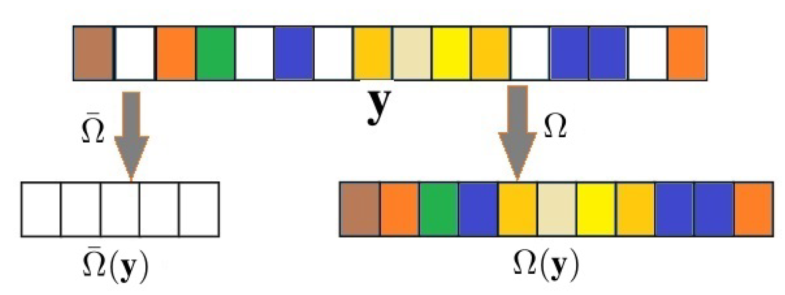
For each patch $\mathbf{y}$ with bleed-through pixels, we select L non-local similar patches within an $N_s\times N_s$ neighbouring window. The similar patches are grouped together in a matrix, ${\mathbf{y}}_G\in {\mathbb{R}}^{p_s\times L}$. In each patch, we have known pixels and missing or bleed-through pixels. Let $\Omega$ be an operator that extracts the known pixels in a patch and $\overline{\Omega }$ an operator that extracts the missing pixels, so that $\Omega \left(\mathbf{y}\right)$ represents the known pixels and $\overline{\Omega }\left(\mathbf{y}\right)$ represents the missing pixels in a patch $\mathbf{y}$. An illustration of such pixels’ extraction is given in Figure 2.

Similarly, for a group of patches, $\Omega \left({\mathbf{y}}_G\right)$ extracts the known pixels of all patches, averaging multiple entries at the same pixel location, and $\overline{\Omega }\left({\mathbf{y}}_G\right)$ represents the missing pixels. Given a well-trained dictionary $\mathbf{D}$, the sparse reconstruction of patches with bleed-through pixels can be formulated as

$$\widehat{x}=arg\underset{x}{min}\parallel \Omega \left({\mathbf{y}}_G\right)-\Omega \left(\mathbf{D}x\right){\parallel }^2+\alpha \parallel x{\parallel }_0,$$

(10)

where $\alpha$ is a small constant. The first term of Equation (10) represents the data-fidelity and the second term is the sparse regularization. After obtaining the sparse coefficients $\widehat{x}$ using Equation (10), an estimate for the bleed-through pixels can be obtained using

$$\overline{\Omega }\left(\mathbf{y}\right)=\overline{\Omega }\left(\mathbf{D}\widehat{x}\right).$$

(11)

Using the reconstructed patches, an estimated, bleed-through free image is obtained by means of patch averaging, according to Equation (9).

In this paper, we learned a dictionary $\mathbf{D}$ from the training set $\mathbf{Y}$ created from the overlapping patches of an image with bleed-through, using the method described in Section 2. For optimization, we used only complete patches from $\mathbf{Y}$, i.e., the patches with no bleed-through pixels, selected from both background areas and foreground text. This choice of “*”clean patches speeds up the training process and excludes the “*”non-informative bleed-through pixels. After dictionary training, the sparse coefficients in Equation (10) are estimated using the OMP algorithm presented in [48]. The order in which the bleed-through patches are inpainted has a significant impact on the final restored image. Thus, similarly to [20], high priority is given to patches with structure information in the known part. This patch priority scheme enables a smooth transition of structure information from the known part to the unknown (bleed-through) part of the patch.

5. Experimental Results

In this section, we discuss the performance of our method in order to validate its effectiveness. We compared the proposed method with other state-of-the-art methods including [7,16]. For evaluation, we used images from the well known database of ancient documents presented in [63,64]. This database contains 25 pairs of recto-verso images of ancient manuscripts affected by bleed-through, along with ground truth images. In the ground truth images, the foreground text is manually labeled. For the proposed method, the input images are first processed for bleed-through detection as discussed in Section 3.

The dictionary training data set $\mathbf{Y}$ is constructed by selecting the overlapping patches of size 8 × 8 with no bleed-through pixels from the input image. We learned an overcomplete dictionary $\mathbf{D}$ of size $64\times 256$ from $\mathbf{Y}$, with sparsity level $\mathrm{m}=5$ and $\alpha =0.26$. We used discrete cosine transform (DCT) matrix as an initial dictionary. For each patch to be inpainted, the sparse coefficients are estimated using the learned dictionary and OMP. The sparse coefficients of each patch, denoted by ${\mathbf{x}}_j$, where j indicates the number of the patch, are then used to estimate the fill-in values for the bleed-through areas. In terms of computational complexity, the dictionary training step comparatively consumes more time. The K-SVD algorithm requires K-times singular valve decomposition (SVD), with computational cost of $\mathit{O}\left(K^4\right)$, where K represents the number of atoms. The proposed method is implemented in the MATLAB2016a platform (The MathWorks, Inc., Natick, MA, USA) on a personal computer with core i5-6500 CPU at 3.20 Ghz and 8 GB of RAM. It took about 2 min for dictionary learning, and 57 s for inpainting an image of $720\times 940$ pixels.

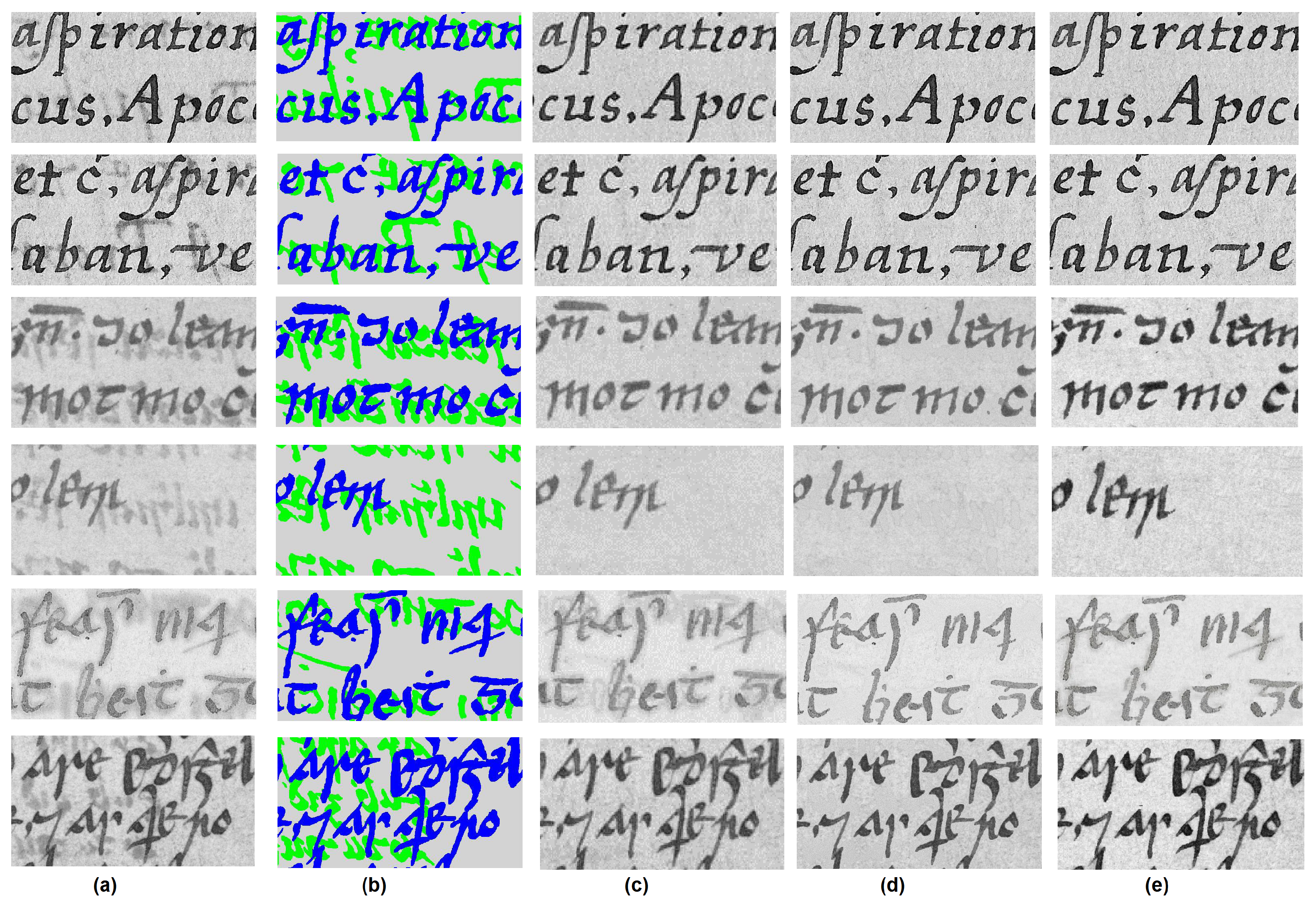
In bleed-through restoration, the efficacy is generally evaluated qualitatively, as in real cases the original clean image is not available. A visual comparison of the proposed method with other state-of-the-art methods is presented in Figure 3. The reported results for [16] are obtained from the online available ancient manuscripts database (https://www.isos.dias.ie/). In the ground truth images, obtained from [7], foreground text and bleed through are manually labeled. As can be seen, the proposed method (Figure 3e) produces comparatively better results considering the given ground truth image. It efficiently removes the bleed-through degradation, leaves intact the foreground text, and preserves the original look of the document. The non-parametric method of [16] (Figure 3c), although retaining foreground text and background texture, leaves clearly visible bleed-through imprints in some cases. The recent method presented in [7] (Figure 3d) produces better results, but some strokes of the foreground text are missing.

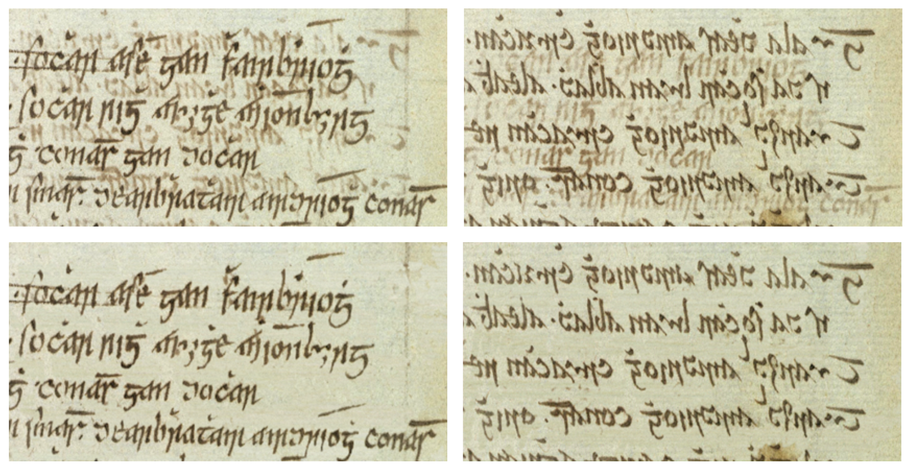
A bleed-through free colour image, obtained by using the proposed method, is shown in Figure 4. In the case of color images, we applied the proposed inpainting method only in the luminance (luma) band, and a simple nearest-neighbour based pixel interpolation is used in the other two chrominance bands. The proposed method copes very well with bleed-through removal and the dictionary based inpainting preserves the original appearance of the document.

6. Conclusions

This paper presents a novel and general framework for high quality image restoration of documents affected by bleed-through. We use the bleed-through identification method presented in [33] in conjunction with group based sparse image inpainting, in order to obtain a non-blind document bleed-through the removal method. The non-stationary linear model in [33] efficiently locates the bleed-through pattern in recto-verso image pairs, but lacks a proper method to replace the unwanted bleed-through pixels. Finding a befitting fill-in for the degraded pixels is a crucial task because the imprints due to assigned values that are not in accordance with the neighborhood have unpleasant visual effects, and destroy the original look of the restored document. The simple replacement with the predominant gray level value of the local background does not solve the problem. To remedy this issue, a non-local group based adaptive sparse image inpainting is suggested to estimate plausible fill-in values to replace the identified bleed-through pixels. The inclusion of non-local similar patches encourages the consistency in local fine textures, without blocking or smoothing artefacts. The proposed image inpainting method efficiently employs the intrinsic local sparsity and the non-local patch similarity. The performance of the proposed method is compared with other state-of-the-art methods on a database of recto-verso documents with bleed-through degradation.