1. Introduction
Image segmentation is a technique of partitioning an image domain into multiple regions such that each region is homogeneous with respect to some characteristic such as intensity, texture and/or color. It is often used to locate objects or to find the respective boundary. It is an active research topic with numerous practical applications. Examples include medical imaging, machine vision and video surveillance. Image segmentation can be very challenging for images with noise, low contrast and multi-scale, multi-directional details. Conducting multiphase segmentation, rather than binary “object vs. background” segmentation in these cases adds complexity to the problem.
Image segmentation has been studied for many years. Methods in the literature include simple intensity thresholding, edge detection-based and clustering-based segmentation, watershed approaches, variational and graph-based techniques. A variety of methods was proven to be efficient for a variety of images (datasets) with different properties. For instance, thresholding [
1,
2,
3] is the simplest and fastest method that works well for images with clearly-defined boundaries between target regions and without significant noise present. The watershed method [
4,
5] tends to be more successful when the objects of interests are closely grouped together and, possibly, touch and share their boundary (e.g., microscopy imagery of cells). It however requires correct seeds for each object to segment [
6,
7,
8]. Image segmentation can be very difficult for images with noise, low contrast and/or multi-scale, multi-directional details. Variational models usually involve solving an appropriate minimization problem, and thus are, on the one hand, more time consuming, yet, on the other hand, are more robust and yield more accurate results due to the regularity and fidelity terms providing clear and numerically-implementable requirements on the output. Many variational segmentation models originate from the Potts model [
9] that minimizes the sum of the boundary length and data fidelity. The Potts model is NP hard in multiphase cases. Graph cut-based models were proposed to approximate global minimizers in computationally-efficient ways [
10,
11,
12,
13,
14,
15]. The Mumford–Shah model [
16] can be viewed as a discrete case of the Potts model that assumes piecewise smoothness of the image intensity.
The geodesic active contour model [
17], Chan–Vese active contour model [
18,
19] and other level set methods represent another important class of techniques that were proposed to improve segmentation efficiency. In particular, the multiphase Vese–Chan model [
19] assumes piecewise constant image intensity and is easier to implement than Mumford–Shah. A method involving
approximations of the total variation by functionals with equispaced multiple well potentials in the context of multiphase segmentation is presented in [
20]. However, due to the nonconvexity of the model, the segmentation results highly rely on the selection of the initial approximation, thus requiring careful practical implementation. Recently, convex relaxation-based approaches have been studied to improve the robustness of segmentation, as well as the computational efficiency [
21,
22,
23,
24,
25,
26,
27]. There is also work focused on multiphase fuzzy segmentation and applied on medical images [
28]. Diffuse-interface models adapted to the graph context were shown to be efficient in binary segmentation for a variety of datasets [
29,
30]. Other not directly related, but effective segmentation methods listed on the Berkeley segmentation dataset and benchmark website include [
31,
32,
33,
34,
35]. These techniques are contour detection oriented and are directly associated with the object vs. background classification.
About our method. As was remarked in [
19], the multi-phase image segmentation problem is different from any binary segmentation task. Our method, just as the above mentioned level set segmentation, by construction avoids the issues of ‘vacuum’ and ‘overlap’; moreover,
m binary functions are enough to encode
-valued piecewise constant approximation. The case when
is considered especially interesting, since, formally, the partition of any piecewise smooth image near any boundary junction can be encoded by only two binary functions, per the four color theorem. Therefore, in our problem setup, we focus on the four-phase image segmentation as a typical case of a problem of approximating a given image by a piecewise constant one, attaining at most four intensity values, with connected components of the output satisfying certain regularity conditions. Those conditions are imposed by the properties of the energy functional we introduce in
Section 2.1.
Our model uses such features of diffuse interface behavior as coarsening and phase separation to merge relevant image elements (coarsening) and separate others into distinct classes (phase separation). To balance these two tendencies, one can adjust the diffuse interface parameter , just as in the classical diffuse interface models that arise in material science. However, in the new spatial derivative-free setup, the interface width is no longer proportional to (due to the well-localized elements in the chosen sparse representation systems and, thus, a completely different diffusive nature of the model), allowing combining the advantages of non-local information processing with sharp edges in the output. Numerical experiments confirm the effectiveness of the proposed method.
This technique is especially suitable for images where the segmented output is expected to have piecewise smooth edges and relatively large connected components (that is determined by the diffuse interface value
and the weights of the fidelity terms; see
Section 2.2) within each segmented class (and nearly no isolated pixels).
Novelty and contributions. Preliminary findings about this approach appeared in the SPIE Conference Proceedings [
36]. In this paper, we do an in-depth investigation of this segmentation model. We provide a detailed description of the numerical scheme and conditions that make it gradient stable; we include the formal proof of the minimizer existence, a detailed description of the fidelity term choice and parameter choice; we also describe generalizations and adaptations of this method for particular applications: using it with post-processing for specific needs of medical imaging (blood vessel detection) and generalization of the method to process color (vector-valued) images, both illustrated with examples of numerical simulations. Moreover, following up on the requests of this journal’s reviewers, we include the quantitative area-segmentation comparisons to other methods (using benchmarks described in [
31] and other works associated with the Berkeley segmentation database(s); please, see
Section 4.1 and
Appendix B.1).
In
Section 1.1 and
Section 1.2, we provide a more detailed explanation of our model design, the reasons for using wavelets or similar multiscale systems in the variational context and briefly describe the properties of the wavelet Ginzburg–Landau energy.
Section 2 and
Section 3 introduce the variational model and its discrete implementation, respectively.
Section 4 contains the results of numerical simulations and a discussion of the effectiveness of our method.
1.1. PDE-Free Variational Models Based on Sparse Representations: Motivation
Similarities between image topology features and phase transitions behavior in material science and fluid mechanics motivated the integration of diffuse interface models into image processing [
37,
38]. These techniques are sometimes based on the phase-field models, such as the one of Modica and Mortola [
39], and allow for topology transition between two steady states of a certain physical or artificial system. Such a construction seems naturally consonant with image processing applications that consider the image intensity bitwise and treat (recover) respective binary values as two equilibria of a model system [
40,
41].
In general, non-linear diffusion models allow the inclusion of a priori knowledge to ensure regularity while preserving important features including edges [
42]. Anisotropic diffusion provides the advantage of combining image regularization with the possibility of edge enhancement [
43,
44].
However, in signal and especially image processing, we deal with discrete signals and spatially localized features, which do not directly fit into the context of differentiation, even in the weak sense, and the Fourier basis, containing the eigen-functions of certain differential operators, does not provide spatial localization. Moreover, Fourier coefficients of a typical image are not sparse.
A logical and elegant resolution of these difficulties lies in constructing a class of operators based on multiscale sparse representation systems, such as multiscale frames (wavelet or other *-lets). These operators can be designed to act on the chosen frame in the same scale proportional manner as the differential operators act on the Fourier basis. It turns out that with a suitable choice of the multiscale sparse representation system, the new operators retain the desired properties of their differential prototypes, while bringing in new advantages, such as being inherently multiscale, well-localized in space and frequency and, for some multiscale sparse representation systems, allowing some control of the directional features. However, even using the most basic systems like 2D separable wavelets yields non-trivial improvement in the diffuse interface imaging techniques.
1.2. Wavelets in Variational Models for Image Analysis and Recovery, Wavelet Ginzburg–Landau Energy
Wavelets are a well-known powerful tool of image processing, primarily for their ability to capture important signal features within a few terms of the wavelet decomposition; significant attention has been devoted to investigating the properties of the sparse representation systems as effective tools of harmonic analysis within new models that better reflect the modern signal processing needs. In this paper, we exploit the intrinsic connections between the classical differential operators and pseudo-differential ones based on sparse representations (already studied in [
45,
46]) in the new context of the segmentation problem where two functions and possibly some additional parameters need to be recovered (via solving coupled systems of evolutional differential equations).
Wavelets were used for image enhancement and recovery in a multitude of variational settings; see [
47,
48] and more. In particular, [
47] discusses the total variation (TV) minimization in the wavelet domain, that successfully reproduces lost coefficients. The relationship between wavelet-based image processing algorithms and variational problems in general is analyzed in [
49,
50].
The wavelet Ginzburg–Landau energy was constructed from the idea of designing new types of pseudo-differential energy functionals that inherit important properties of the ones involving derivatives, introduce the advantages of non-local analysis of the image features and leave out the computational drawbacks associated with the discrete differentiation.
The key idea in the design of wavelet Ginzburg–Landau (WGL) [
45,
46] combines the basic geometric framework of diffuse interface methods with advantages of the well-localized and inherently multiscale wavelet operators. It originally appeared in a variational model that was adapted to a wavelet setting with the goal of using it for image inpainting. However, it is an efficient regularizing term, and it was shown to be successfully used in multiple image analysis and recover settings with properly chosen forcing terms.
The analytical properties of the wavelet Ginzburg–Landau (GL) energy and its imaging applications are described in detail in [
45,
46]. We present a very brief summary below.
Here and further in the text, whenever the domain of integration is omitted, we assume integrating over the entire domain of the respective functions.
The total variation (TV) seminorm was proven to be a natural and efficient measure of image regularity [
51,
52]. However, in many imaging applications, one would like to retain its advantages while making the processing non-local and reduce the computational load related to the curvature calculations. The problem can be re-formulated using the phase-field method providing approximation to the TV functional (in the
sense). The Ginzburg–Landau (GL) functional,
is a diffuse interface approximation to the total variational functional
in the case of binary images [
39,
53].
GL energy is used in modeling of a vast variety of phenomena including the second-order phase transitions. However, if used in signal processing applications, diffuse interface models tend to produce results that are oversmoothed comparing to the optimal output. In the new model, the seminorm is replaced with a Besov (1-2-2) seminorm. This allows one to construct a method with properties similar to those of the PDE-based methods, but without as much diffuse interface scale blur.
The “wavelet Laplace operator” was defined by having the wavelet basis functions as eigenfunctions and acting on those in the same “scale - proportional” manner as the Laplace operator acts on the Fourier basis. Given an orthonormal wavelet
, the “wavelet Laplacian” of any
is formally defined as:
Then, the “wavelet Allen–Cahn” equation
describes the gradient descent in the problem of minimizing the wavelet Ginzburg–Landau (WGL) energy:
is the square of the Besov 1-2-2 (translation-invariant) semi-norm if the wavelet
is
r-regular,
. The same exact energy construction (
3) works just as well in the 2D case (in the case of the separable 2D wavelet basis, one needs to include summation over all types of coefficients: ‘horizontal’, ‘vertical’, ‘diagonal’, in the above formulas).
WGL functionals are inherently multiscale and take advantage of simultaneous space and frequency localization (due to the wavelet properties), thus allowing much sharper minimizer transitions for the same values of the interface parameters compared to the classical GL energy.
WGL energy does not have any local maxima, but a local minimum can be found via the gradient descent method. The latter problem is equivalent to solving:
The above problem is well-posed: it has a unique solution that exists globally in time and converges to a steady state as . The steady state solution is infinitely smooth provided that wavelet used in the construction of the energy has sufficient regularity.
The WGL energy approximates a weighted TV functional in the variational (-convergence) sense.
The WGL was initially designed for the recovery of binary signals; however, it is easily adaptable to a wide class of imaging applications via bit-wise processing ([
40] and more).
Variational techniques with WGL as the regularizer were developed for such problems as inpainting, denoising, superresolution, segmentation and more [
45]. In all of those cases, the minimized energy was respectively modified to include one or more fidelity terms suitable for each type of problem. When used for the purposes of (binary) segmentation, the input of the method was assumed to include “partial classification” of the image into two classes, and the variational model “filled in the gaps”: the diffusive nature of the model allowed propagating the information, and the edge-preserving term enforced the boundaries of the objects.
The model we introduce in this paper is different from other WGL-based ones in several ways. In the new model, we recover a more complicated output: the binary functions that define the separation of image pixels into classes and the values of constants of the piecewise constant approximation within one unified procedure. It is achieved by solving the system of ordinary differential equations associated with the gradient descent minimization of the proposed energy functional.
2. The Proposed Model for the Four-Phase Image Segmentation
2.1. The Problem Setup
Let us denote the original image
f and assume it is a function from
. We are looking for the four-phase segmented version of the given image, i.e., its nearly piecewise constant approximation in the following form:
Function u is, by design, a piecewise constant function attaining four possible values , , , , and functions and are binary (take on values of zero and one). For simplicity, let us assume that . Since our method is a diffuse interface, the recovered functions will be nearly binary, such that the width of the transition between black and white is comparable to the size of one pixel.
We assume that the desired function
u can be obtained by minimizing the following energy:
with respect to functions
and
, as well as
. The minimizing functions
,
are expected to be nearly-binary functions from
. The fidelity part of the energy consists of two terms. The term
ensures the mean-square proximity of the resulting piecewise constant output
u to the original function
f. The edge-preserving term
takes care of retaining the most important edge information: here
is the subset of the wavelet modes in the wavelet decomposition that are significant enough to be preserved in the segmented version of the image; one of the possible ways of choosing
is described in
Section 4. The values
and
are weighting parameters that are chosen depending on the image quality, detail resolution and amount of reliable edge information that needs to be preserved. The seminorm
denotes the Besov 1-2-2 seminorm (just as in (
3)).
The existence of minimizers for
E can be proven using a standard compactness argument (see
Appendix A.1). The minimizers are not unique (the easiest counterexample is a constant input function). The output of our numerical simulations depends on the initial guess, which allows us to steer the solution in the desired direction. We provide details about the initialization procedure in
Section 3.2.
2.2. Motivation for the Energy Design
The main objective of any image processing method is to successfully incorporate all of the known data properties and requirements on the output into a tunable mathematical model. In variational models, the terms of the minimized energy often are categorized as either regularizing or fidelity (forcing) terms. Let us explain the features of the above energy in relation to our segmentation goal.
In our case, the pixels in the output image will be inadvertently grouped into colored connected components. Each of such components should have a reasonably regular geometric structure (due to the influence of the regularizing WGL terms) unless otherwise imposed by the edges of the original image (due to the influence of the edge-preserving and/or spatial fidelity terms). The values of the functions and are also expected to be nearly binary.
The terms and represent the regularizing part of the energy. They bring in the properties of the diffusive model inherited from the classical second order phase transition ‘coarsening’ and ‘phase separation’, which facilitate the needed evolution within the image: merging relevant image elements (coarsening) and separating others into distinct classes (phase separation). To balance these two tendencies, one can adjust the diffuse interface parameter , just as in the classical diffuse interface models that arise in material science. However, in the new spatial derivative-free setup, the interface width is no longer proportional to (due to the well-localized elements in the chosen sparse representation systems and, thus, a completely different diffusive nature of the model), allowing combining the advantages of non-local information processing with sharp edges in the output.
For each of the functions , we aim to minimize WGL, thus making their supports somewhat regularly-shaped (due to the coarsening tendency) and their values nearly binary (due to phase-separation).
The fidelity components of the energy are . These terms impose consistency with the original image f in the sense and preserve significant edges within the original image.
If the piecewise constant approximation values are known in advance, the simplified version of this algorithm can recover the corresponding regions by finding
and
. However, in general, the coefficients
are not defined in advance and cannot be easily recovered from the histogram analysis of the image values, as shown in
Appendix A.2. In the rest of the paper, we assume that
is unknown, and in all of our numerical experiments included in this paper, we recovered
,
and
simultaneously.
In the rest of the paper, we will show that our method provides a powerful tool of using diffusive (in the alternative sense of gradually suppressing the high scale detail in the context of a multiscale multidirectional representation system such as wavelets) propagation of information without the associated blurring. The trade-off between preserving the fine-scale features and connecting all relevant components is resolved by using the forcing terms, including the edge-preserving term, obtained by the specialized scale-dependent thresholding.
2.3. Solving the Minimization Problem
We look for , , the minimizers (local) of the energy (4), as well as for the the coefficients , if those are not fixed in advance.
Let for convenience in writing the gradient descent equations. We can do so because we are assuming that the range of values of the image is non-negative; thus, the optimal approximation values (even in the case of noisy images) are non-negative.
Consider a variation of this energy at a point
in the direction
:
Here,
,
, and:
We look for the minimizers of the chosen energy functional as the steady state solutions (in the weak sense) to the gradient descent system:
Here,
and
for any
.
Our method has a non-local nature as the equations defining the minimizers (
) contain a non-local operator (
), thus allowing creating better connections between components of the segmented image. Interaction of the diffusive term that facilitates merging of similar-colored regions and the term minimizing the double-well potential, i.e., responsible for keeping functions
nearly binary, closely resembles the “coarsening” and “phase separation” attributes of the classical Allen–Cahn equation. However, due to the wavelet-based operator we use instead of the Laplacian, we can achieve better phase separation and, thus, narrower black to white transitions even while requiring larger connected components in the output. In other words, larger values of parameter
indeed facilitate the diffusion process that merges more pixels into one connected component, yet the the loss of contrast (i.e., increasing the width of the black to white transition) is most certainly less noticeable than in diffuse-interface methods based on the classical models involving diffusive differential operators. These features were investigated in detail in [
45].
The edge-enforcing component enhances the recovery of more precise boundaries of the segmented regions. The spatial consistency term naturally enforces the proximity between the input image and its segmented version.
Since our model is variational and any minimization process involves an initial guess, we describe one of the possible ways to choose the initial values in
Section 3.2.
3. Numerical Implementation
3.1. Numerical Scheme
To compute the minimizers of the proposed variational problem, we implement the gradient descent method described in
Section 2.3 via a semi-implicit numerical scheme. To guarantee gradient-stable convergence to a steady state (for functions
), we use the convexity splitting scheme from [
54]:
, where:
Here, the constants need to be chosen in such a way that all four energies are convex, making E a difference of strictly convex energy functionals. If , it can be achieved by choosing and . If we consider only the “continuous, non-discretized” form of the energy, the needed , generally speaking, does not exist. However, in the discretized form, all functions involved in the gradient descent are represented by matrices; therefore, only finitely many levels of wavelet decomposition are present in the Besov seminorm in the fidelity term; thus, we may choose , where is the maximum level of wavelet decomposition possible for matrices of the chosen size.
Let us describe the discretized version of the gradient descent system. The gradient descent is performed with respect to an artificial time parameter t. Let denote the time step size, then after n steps of the gradient descent algorithm. Let the spatial domain be represented by the points on the uniform grid of size with step h: , , , , . Due to the use of the discrete wavelet transform, it is convenient to pick , . Let denote a matrix that approximates the values of the at time , and is defined accordingly, so . Naturally, we assume that the given image f is a matrix with entries .
If the intensity values of the output are not fixed and, thus, we update at each step as well, we let denote the value of the intensity vector after n steps of the gradient descent algorithm.
For the semi-implicit numerical scheme implementing the equations of the gradient descent system, we formulated the above results in the following equations:
If the expected constant intensity values of the output image are not known in advance, they can be computed simultaneously with the segmented region defining functions
:
To update functions and , the operators on the left-hand side of the respective equations are inverted in the wavelet domain. In the actual numerical simulations, we use the stationary wavelet transform (redundant, undecimated wavelet transform) due to its translation invariant properties that are pivotal in image processing (especially when dealing with natural images having no intrinsic dyadic structure).
3.2. Initialization
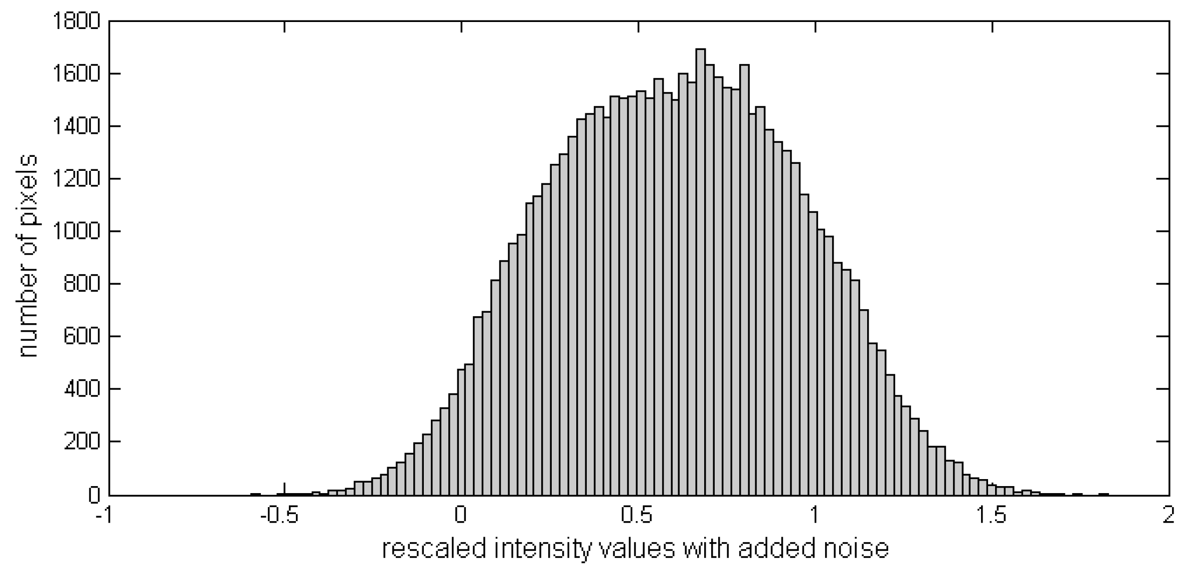
We rescale the range of the intensity values for each processed image to the interval for convenience. In particular, it simplifies the description of feasible ranges for the fidelity weights: should be of the same order as , and should be comparable to , where is the maximum level of wavelet decomposition used in the edge-preserving fidelity term (see more details in the next subsection). In cases when the input image is known to have a significant level of noise present, we rescaled the values and discard the furthest outliers at the same time, namely cut off the lowest and highest of the value range.
The initial guess for the gradient descent system is provided by a simple procedure involving preliminary intensity value distribution analysis of the processed image. A faster convergence can be obtained if the initial guess is provided by the k-means algorithm, which, however, is more computationally expensive, so it is not the best choice of the initial guess. Nevertheless, it is worth mentioning that our algorithm, among other things, can be efficiently used as a post-processing routine following k-means segmentation with the purpose of reducing the number of connected components in the output and regularizing their boundary. We discuss this in the context of color image classification in
Section 4.3.
Appendix A.2 provides more comments on the choice of the initial guess for
.
Here and further in the text, we will use the percentile function:
The initial values of the coefficients
can be assigned somewhat uniformly from the range of the given image intensity values; we typically took:
,
,
,
(just as earlier, we assume that
f is the given image represented by a matrix
with entries
). Then, the preliminary segmented domains can be determined by their indicator functions (matrices) as follows: for
and any pixel position
:
then:
The initial value of the approximating piece-wise constant function
u then is
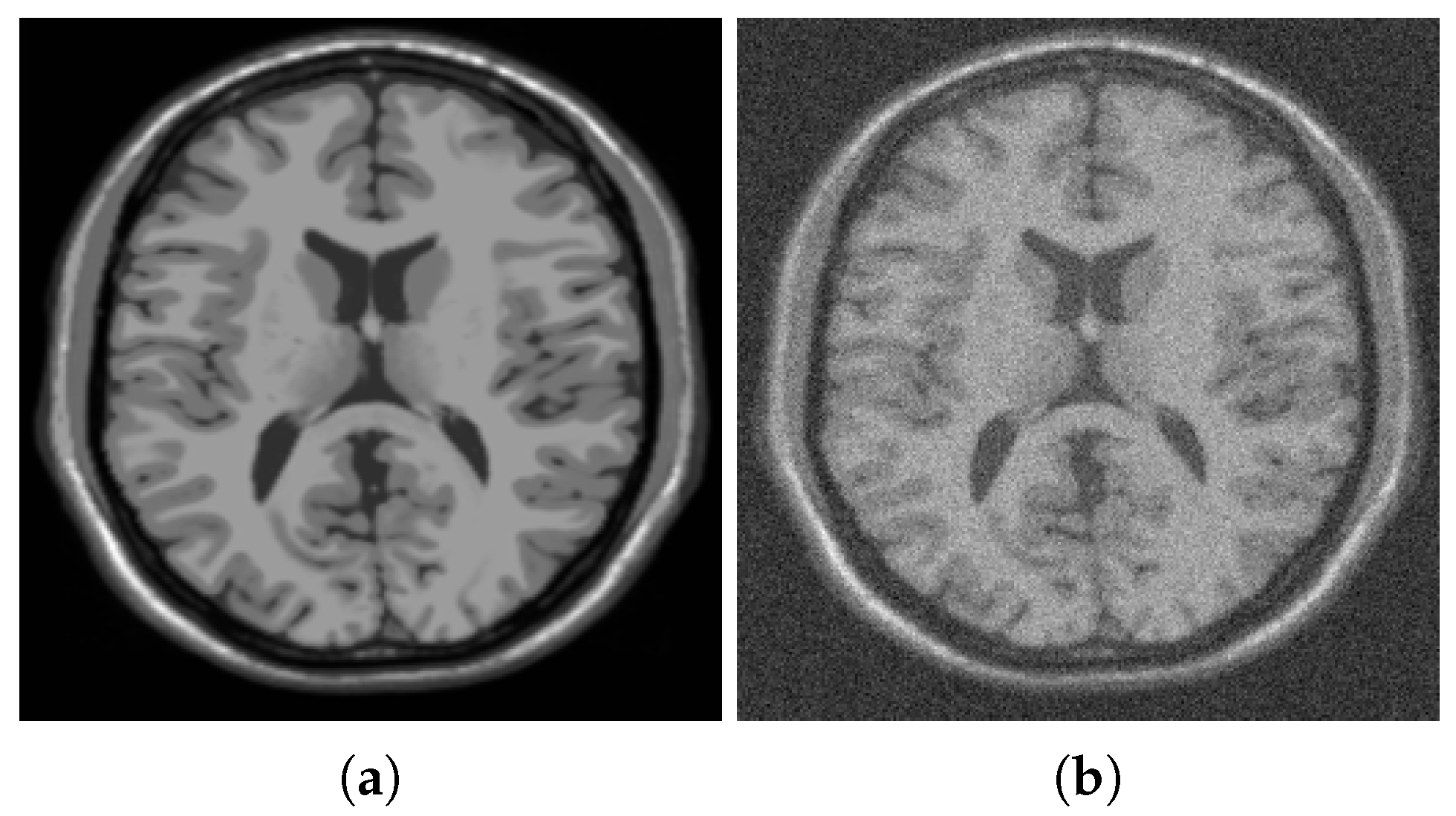
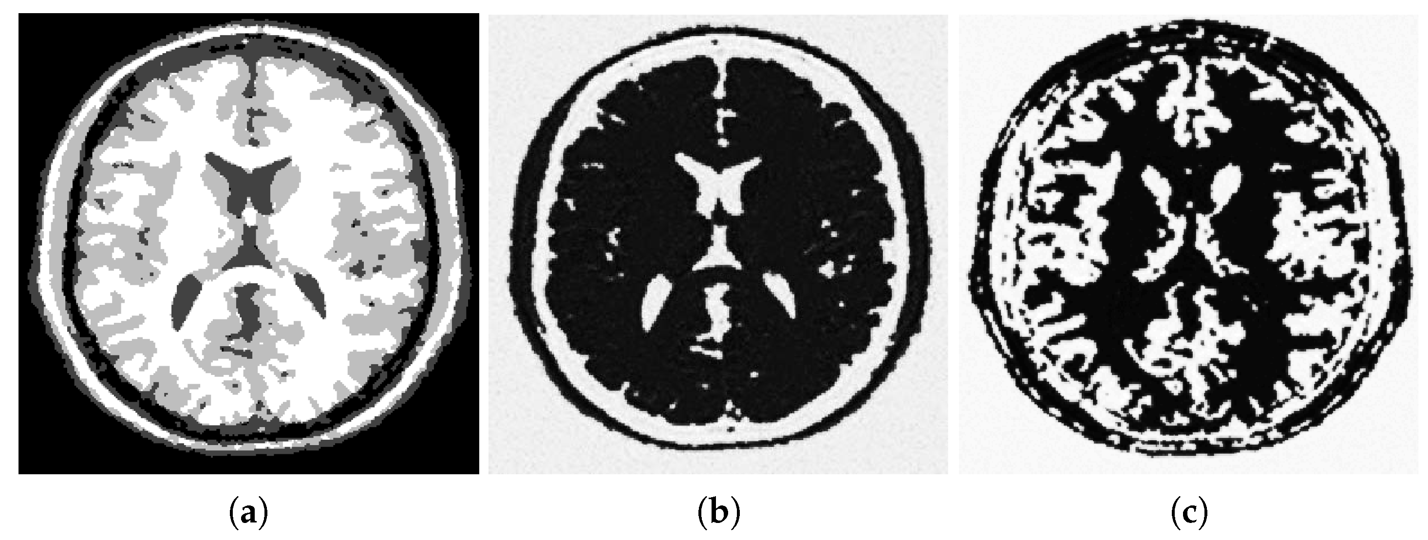
. An example of such initialization for the image in
Figure 1b is shown in
Figure 2b,c.
3.3. Choosing the Edge-Forcing Term
The fidelity term
is responsible for preserving the main set of edges associated with a subset of wavelet modes that we denoted
. The wavelet modes that are “significant” in the segmentation of a given image are found in the same adaptive thresholding algorithm that was previously described in [
45]. Even though the thresholding approach was originally designed for binary images, it works well in detecting the edges that are ‘locally binary’, i.e., rapid jumps from one nearly constant intensity region to another. Here is a summary of the thresholding procedure we use to determine the edges that correspond to significant intensity jumps and, therefore, to define
.
The redundant (i.e., stationary or undecimated [
55]) wavelet transform of an image
f (
) produces four matrices of coefficients: approximation, horizontal, vertical and diagonal at each level of decomposition, each matrix of the same size as the original image. Let
formally denote coefficients of the wavelet decomposition of
f, indexed by the scale (i.e., dilation parameter)
j, translation
and the ‘type’ of the coefficient
. For any index
,
,
with
and
is ‘a’, ‘h’, ‘v’ or ‘d’, and
is the maximum depth of decomposition (number of scales in the decomposition).
We define the subset
of significant modes as follows. For any image, depending on its size and quality, we may decide to preserve only significant coefficients of scales within a certain range:
(notice that in our notation, the scales increase from coarsest to finest). If the image contains significant amount of noise, it makes sense to choose
. It does not make sense to preserve the approximation coefficients of the coarsest level; sometimes, it is convenient to disregard one or two coarsest scales of decomposition completely. Within the chosen range of decomposition scales, we pick the significant modes as follows:
where
denotes the standard deviation computed over the set of all coefficients of scale
j, within the ‘type’
subset, if
‘h’, ‘v’, ‘d’.
If ,
The constant coefficient used in this scale- and data-dependent thresholding technique helps produce the best results when chosen individually for each image, but most typically has order .
We illustrate the performance of the method as well as technical nuances leading to the best results in the next section. For example, in the segmentation of the image in
Figure 1b we used the edge-forcing term defined by the edges shown in
Figure 2a; the set of respective coefficients was obtained by the procedure described above. The images representing the edge information used in our model in the processing of other images can be found in
Appendix B.2.
The design of the model and numerical experiments indicate that one should not use the edge fidelity term at all or at least not as a dominating fidelity term, in the cases of smooth images with no visible edges or very noisy images where noise can interfere with the edge detection. Whenever the edges are present, while the noise is relatively mild, it makes sense to use the edge fidelity term, as well as the spatial term, with equal or comparable weighting coefficients.
4. Results
4.1. Four-Phase Segmentation of Grayscale Images
Our numerical experiments involve images from several commonly-considered classes: natural, artificial (cartoon-like), medical (MRI) and images from those categories corrupted by noise and blur. We show that our variational multi-phase segmentation approach can efficiently segment various images, including the tough noisy and blurry images with edges of various scales and directions and even harder ones with low contrast.
Highlighting the previously-mentioned feature of the model, a more relaxed dependence on as the diffuse interface parameter comparing to the classical PDE-based models, let us remark that in our numerical examples, a typical value of is of order and is always greater than (assuming is the size of the segmented image). It facilitates the wavelet-based diffusion that forms components of reasonable scale with a piecewise smooth boundary, yet the actual black to white transitions are far from blurry and have a width that is small enough to leave no artifacts after thresholding (if necessary).
To further illustrate the method’s effectiveness, we include the outputs of three other related segmentation techniques: the Vese–Chan multi-phase method [
19], a graph cut method [
14] and a fuzzy segmentation method [
28] for comparison.
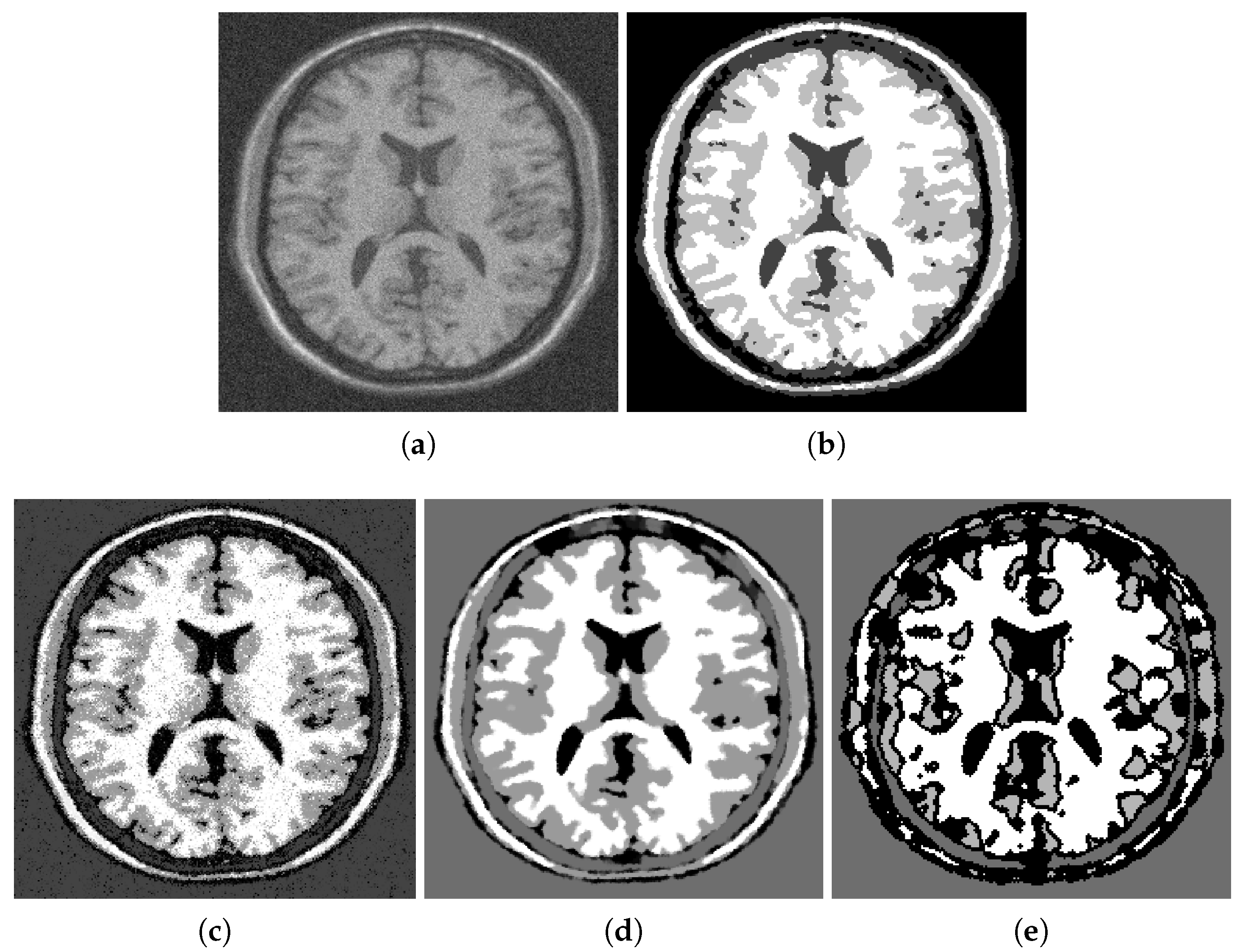
Figure 1,
Figure 2 and
Figure 3 illustrate segmentation of a noisy MRI image (
Figure 1b) that contains many fine details. Specifically,
Figure 2 shows additional details concerning the initialization of the gradient descent minimization and the choice of the edge fidelity term. The MRI image has a size of 256 by 256; the parameters used in simulations are
,
,
.
Figure 4 shows the output of some well-established segmentation methods applied to the same noisy MRI image. Visual examination of the segmented images demonstrates that the fuzzy segmentation result still has noise in its output, and the Vese–Chan method mostly captures the big scale regions. Only the proposed method and the graph cut methods can provide accurate separation of white matter (shown in white), gray matter (shown in gray) and the rest, which contains either cerebrospinal fluid or the background (shown in darker shades). The results of the graph cut and the proposed method are very similar. However, a zoom-in shows that the proposed method recovers more details in the white matter region. It is especially noticeable in the lower parts of the image.
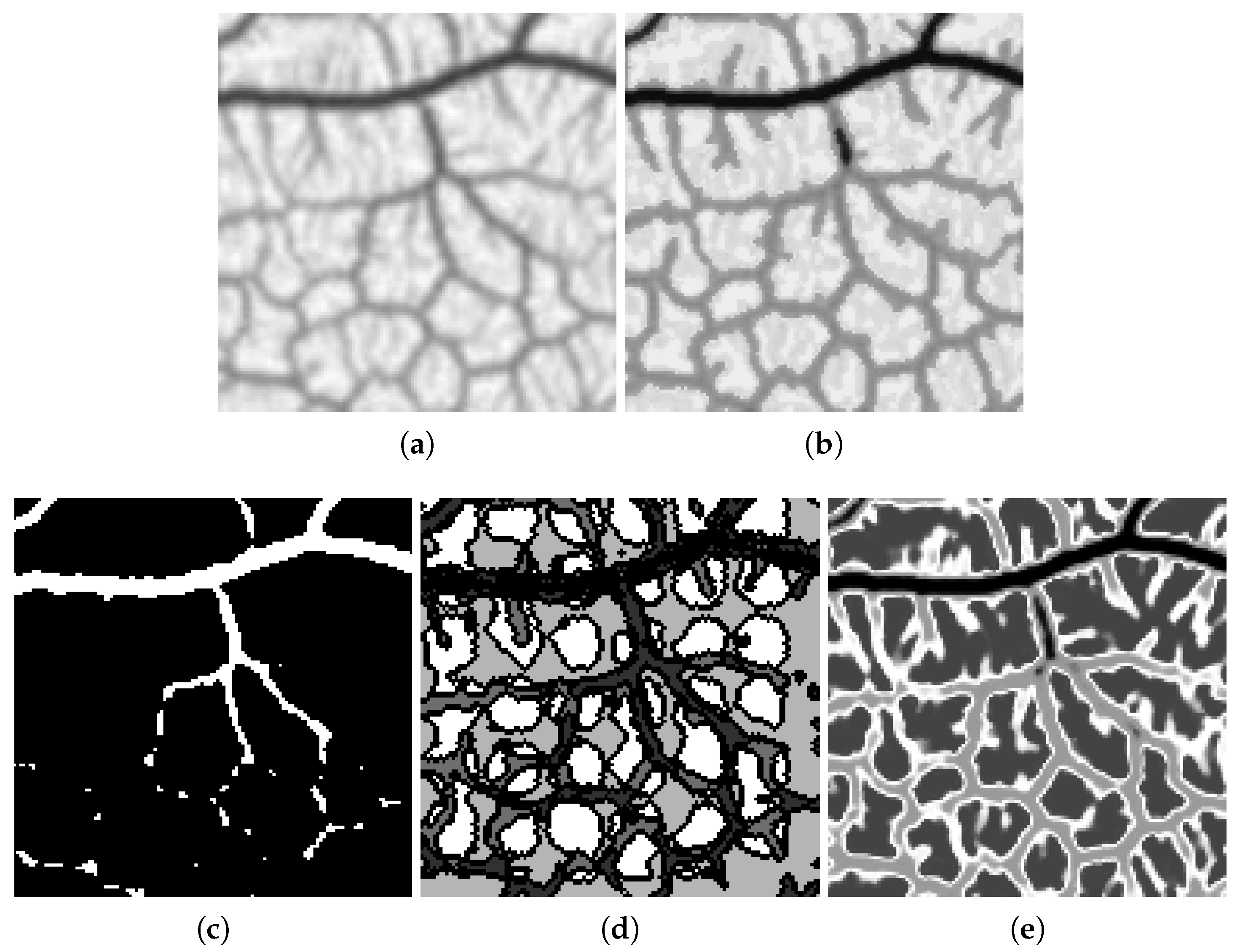
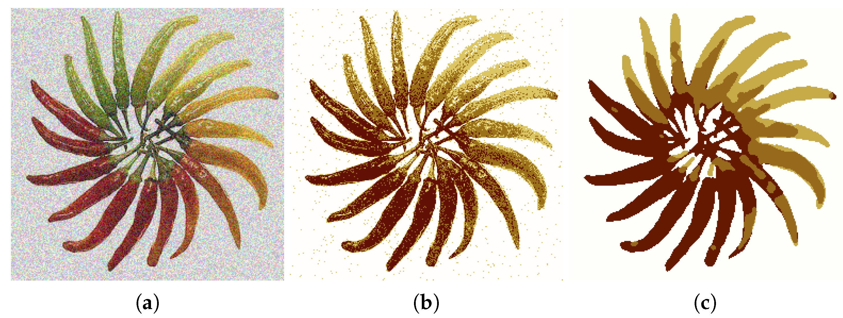
Figure 5 illustrates the fact that the proposed method was the only one that was able to segment the veins of a leaf compared to others. The graph cut method was only able to segment the primary vein while leaving smaller ones out. The four-phase Vese–Chan method was stuck at a local minimum and failed to produce a reasonable segmentation. Somewhat similarly to the graph-cut approach, the fuzzy segmentation segmentation algorithm did well in segmenting the big scale veins, but failed to detect the smaller ones. The ‘Leaf’ image has a size of 128 by 128; the parameters used in simulations are
,
,
.
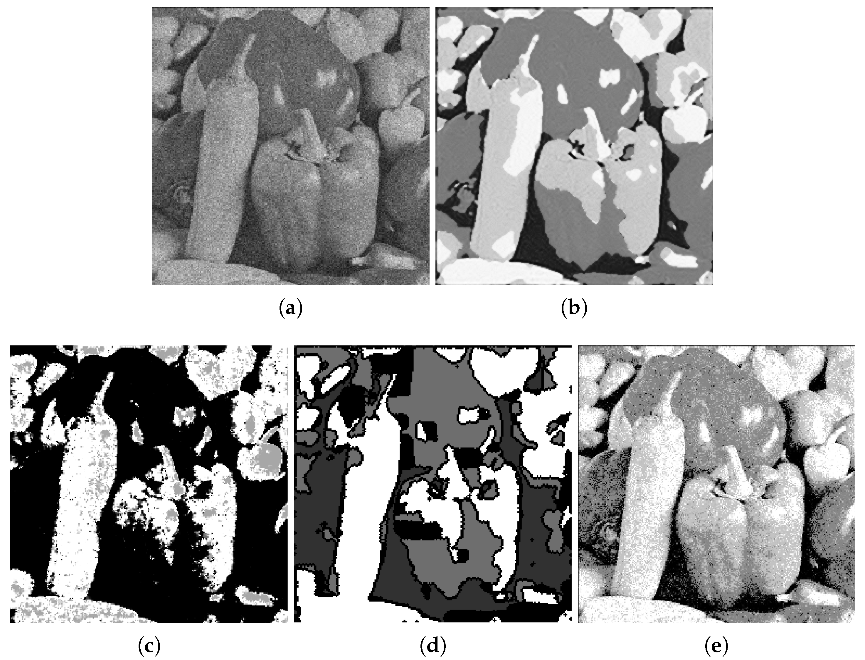
The noisy ‘Peppers’ image in
Figure 6 is a tricky one to segment due to inhomogeneous illumination. The two large peppers in the middle have very bright spots. The segmentation result of the proposed method is more consistent with human perception. The graph cut and the fuzzy segmentation results have leftover artificial noise, while the Vese–Chan method fails to segment the image into four classes. The parameters of simulation were similar to the ones used for the MRI image except for the edge fidelity that had to be decreased due to the noise present.
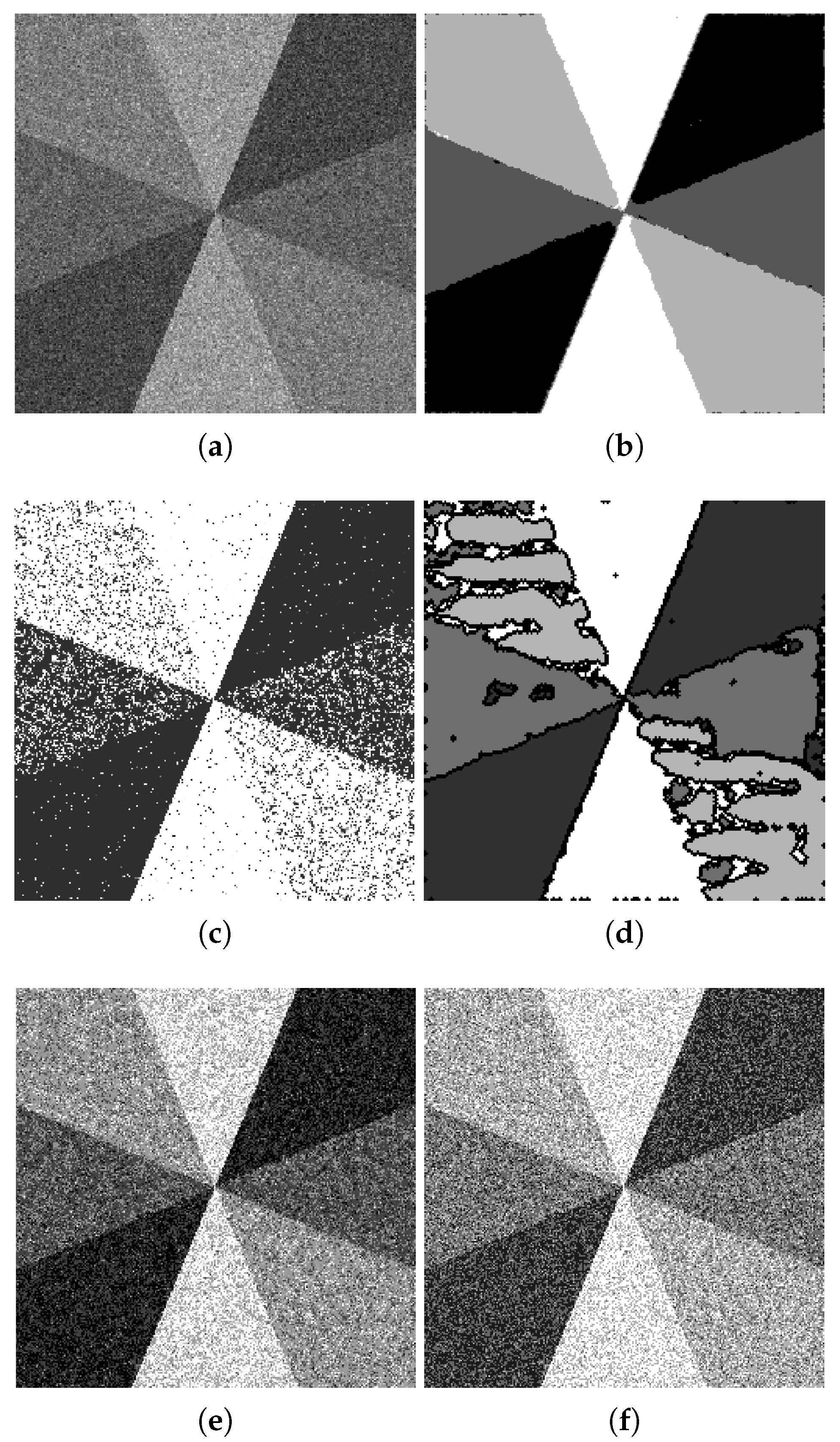
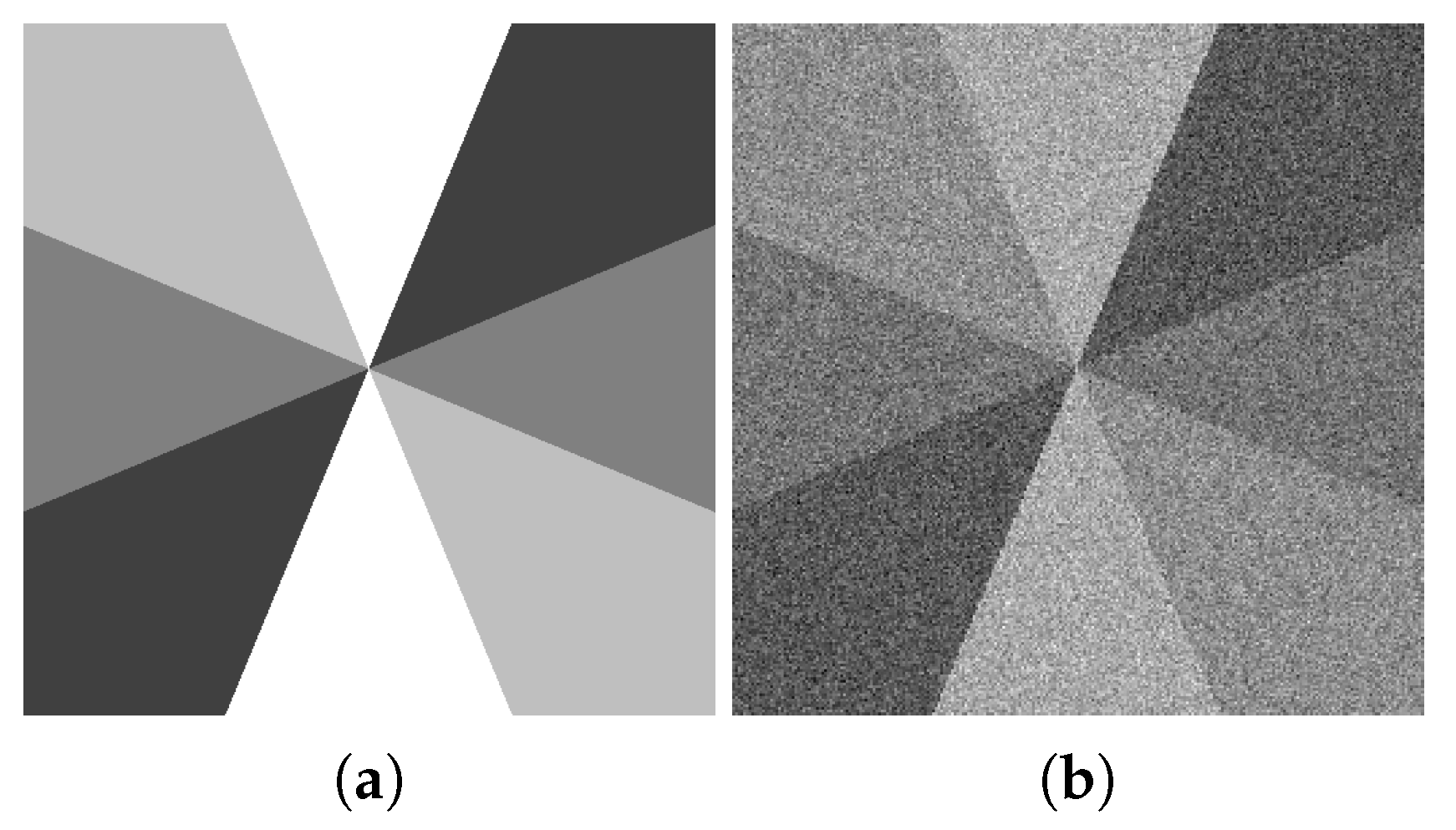
Our next numerical segmentation example is segmenting a four-color grayscale image after adding various levels of noise to the original image ‘Sectors’ is shown in
Figure 7. Without any noise present, the segmentation precision is more than 99.9% (of pixels are classified correctly), and the vector of constants
is recovered within <0.05% of the actual values.
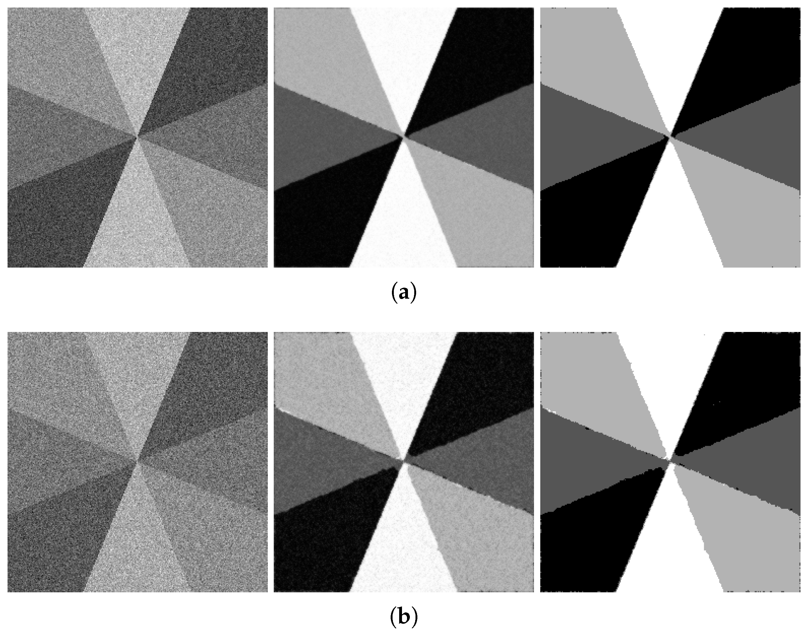
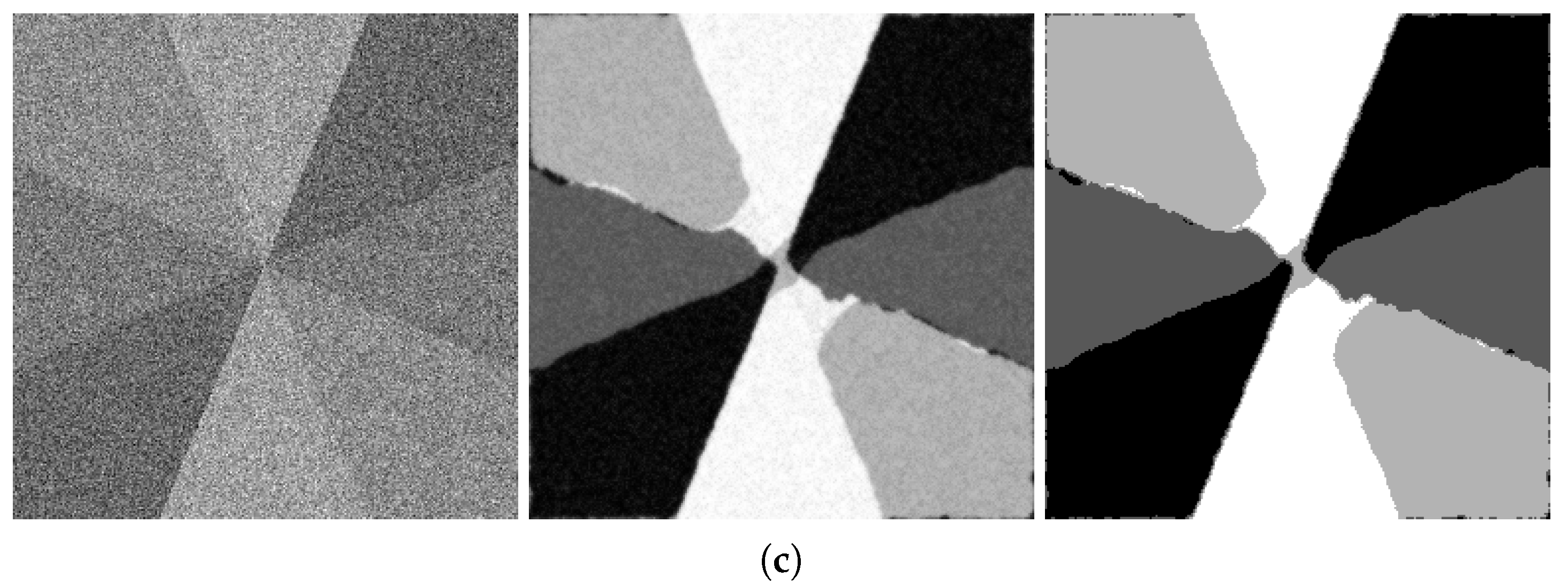
The robustness of our segmentation method to noise is illustrated in
Figure 8: the three images in each row show the noisy input image, direct output of the minimization routine and the result of rounding it to the nearest of the four recovered values
. The rows correspond to the increasing levels of Gaussian noise added to the original image: 15 dB, 10 dB and 5 dB. The figure caption also contains information about the percentage of correctly-classified pixels.
As the noise level increased, it was necessary to decrease the weight of the edge fidelity term and increase the spatial weighting term. For the ‘Sectors’ image with added noise of SNR = 10 dB, the simulation parameters were
,
,
. As was mentioned in
Section 1.2, the WGL energy is not anisotropic. However, for practical purposes, this anisotropy is not affecting the minimization results in any significant way. It is clearly not an issue when we process natural images, where one cannot visually discern straightforward directional patterns. The performance of the method on test images, such as the ‘Sectors’ example, which contains radial edges at a variety of angles, shows the absence of the impact of the WGL anisotropy on the recovery quality. Since the ground truth segmentation for this image was available, our method’s performance was also evaluated with respect to such benchmarks as the Rand index, variation of information and segmentation cover (described in Section 2.3 in [
31] and characterized as appropriate methods for evaluating region-oriented, rather than contour-oriented benchmarks); see
Table 1.
Figure 9 shows the comparison of our method with others when applied to the ‘Sectors’ image with a noise level of 10 dB. We see that the graph cut method could not fight the relatively high level of noise, and the result is still polluted with it. The k-means output is also extremely fragmented. The four-phase Vese–Chan method ended up at a local minimum far from the desired output. The fuzzy segmentation method output looks fine except for the noise still noticeable all over the output image. The same holds for the graph-cut technique.
The quantitative comparison is provided in
Table 2 below.
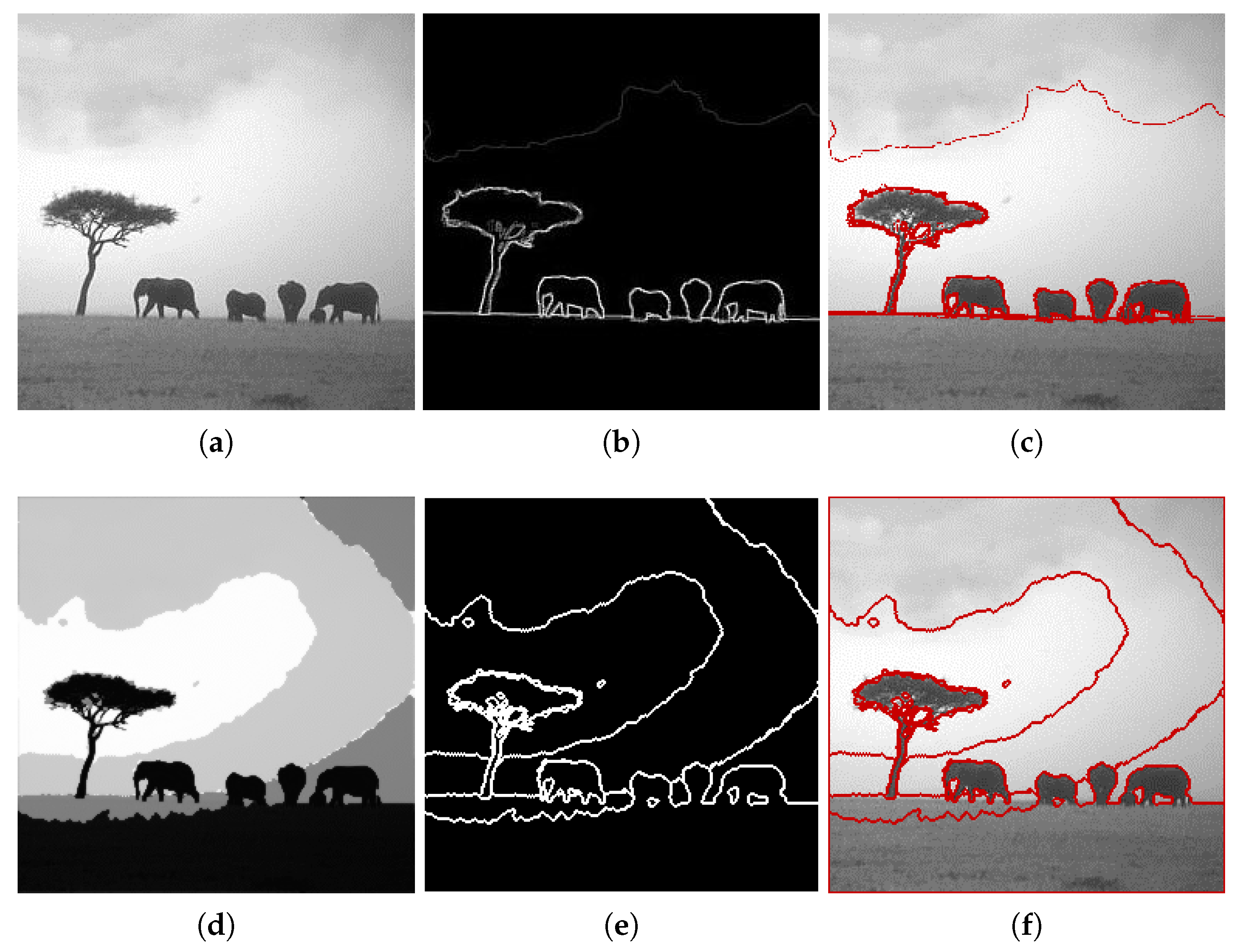
We include the segmentation results of some images from the Berkeley segmentation database ([
33]); see
Figure 10. Additional examples are discussed in
Appendix B.1 and are shown in
Figure A2 and
Figure A3. However, it must be noted that our method is not designed to address the problem of object vs. background detection. It is aiming at classifying the pixels of an image into classes while balancing out the requirements on the output such as the mean-square color similarity within one class, preserving the chosen edges from the original image and the “driving force” of the method: the phase separation and coarsening that lead to grouping pixels into major connected components with a piecewise smooth boundary.
We performed tests on images of sizes
(for the convenience of applying the wavelet transform), for
n = 7, 8, 9. Depending on the image and the choice of parameters, the simulation (which aims at achieving an energy minimizing steady state, i.e., finding a local minimizer) might require between 100 and several hundreds of iterations. The simulations were performed using a PC (Win 7) with Intel i5-3570K CPU 3.40 GHz, 8 Gb RAM, operating system Windows 7, in MATLAB with no parallel computing optimization in our code. It takes about 30 s per 100 iterations for a 256 by 256 image with the maximum level of wavelet decomposition (five scales) w.r.t. the Daubechies-four wavelet (‘db4’). The processing can be significantly sped up by preprocessing, such as preliminary denoising, but we are not addressing this issue here; all simulations were initialized automatically as described in
Section 3.2.
4.2. Blood Vessel Detection in Medical Images
The detection of blood vessels has been an important problem for a while. Most of the successful algorithms are based on machine learning and require a training set of images of comparable quality for successful processing ([
56], and many other publications).
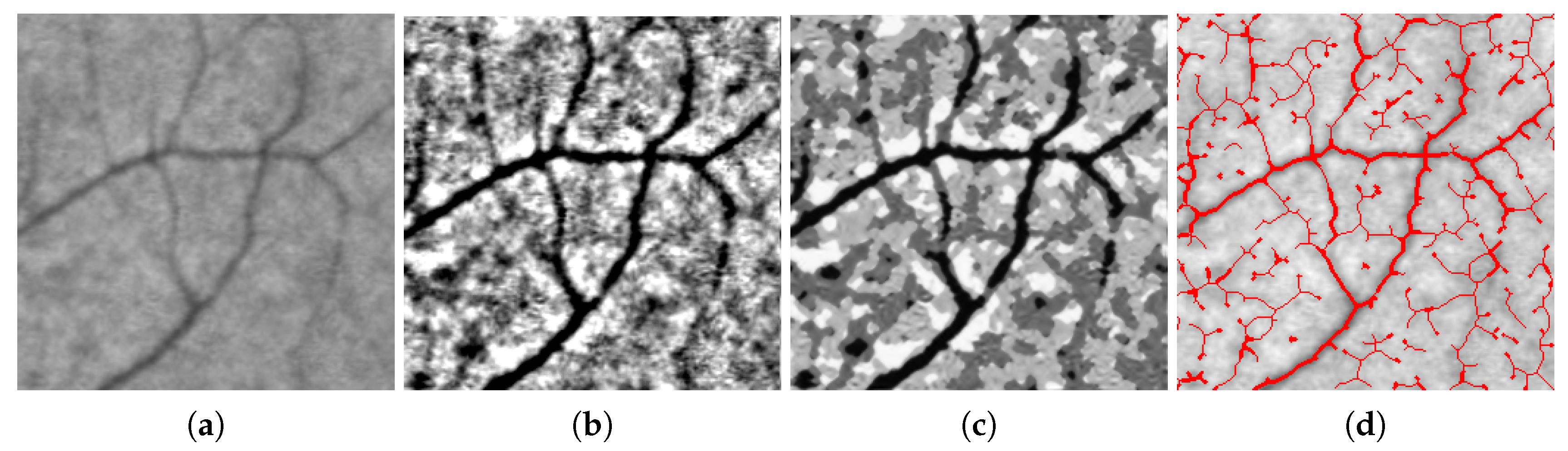
The output of our segmentation algorithm applied to an image with clear detalization (see
Figure 5a,b) shows the advantage of the multi-phase segmentation applicable to the blood vessel detection, since the vessels can actually belong to two classes out of four classes due to highly variable intensity over the entire image. In a way, the detection becomes about the contrast of the blood vessels versus the background, rather than relying purely on the image intensity values. Here, the edge preserving fidelity term plays an important role. However, the images of leaves with clearly pronounced vessels are different in quality from the bio-medical images that typically contain blood vessels. The detalization in bio-medical images is often much worse due to the difficulties of non-invasive acquisition.
A good example is provided by retinal images, where the detection of blood vessels is sometimes needed to exclude the respective pixels from consideration during automatic or semi-automatic processing (for instance, the ratio of intensities at the green and yellow frequencies provides a reasonable estimation for the density of macular pigment, useful in the diagnostics of age-related macular degeneration [
57]).
We consider two examples of our segmentation algorithm applied to retinal images.
The first image we process is a cut-out from a relatively high resolution image, and the capillary structures captured there are barely visible, just because the actual size of those vessels is small relative to the image resolution. The second image contains blood vessels of more various scales, and thus, the corresponding pixels vary more in intensity.
To ‘even out’ the background, we preprocessed the images by removing the coarsest component of the wavelet decomposition:
In terms of practical implementation, we ‘zeroed out’ the coarsest approximation coefficients in the stationary wavelet decomposition of each image. Now, we can expect the blood vessels to be contained within the set of pixels of the two darkest shades of the segmented image, i.e., those with intensities and .
Due to the fact that some components of the segmented outputs are actually wider than the blood vessels, thus merging capillaries with shadows or parts of uneven background, we use the “skeleton” feature of the MATLAB morphological function for binary processing, thus extracting the central line of each component of the set with the characteristic function we detected from the gradient descent output:
. To emphasize the center lines corresponding to the darker segments, we widened them, as shown in
Figure 11d.
4.3. Color Image Segmentation
Color image segmentation falls into a more general category of vector-valued image segmentation, which has been studied for a while. As was mentioned in the Introduction, each segmentation task has its consistency requirements and the expected output properties. We extend our technique to the color images with the purpose of obtaining an output with a certain lower bound on the size of connected components of segmented regions and the piecewise regularity of the boundary of those connected components.
In the case of color image segmentation, the initial guess becomes even more important (due to the general non-convexity of the minimized energy and the increased complexity of the domain of ). Furthermore, it becomes impossible to set the initial condition by elementary percentile-based thresholding; therefore, we propose to use our method as a refining ‘post-processing tool’, after obtaining the initial guess by some relatively simple method like k-means. The “crude” method provides a guess that is somewhat correlated with the desired output , , and our variational method refines its output by running the gradient descent algorithm minimizing the energy E we introduced earlier, thus producing a refined output. We chose to use k-means for obtaining the initial guess because of its straightforward relation to our energy: applying k-means is equivalent to minimizing the spatial fidelity term .
For simplicity, we assume that the input color images are square and are provided in the RGB format; thus, we are to process a 3D array
I of a size
of real values
, where
is the spatial pixel coordinate,
is an integer index between one and three corresponding to ‘red’, ‘green’ or ‘blue’, respectively. We interpret the color image
I as the set of values of a function
f:
. Just as in the 2D case, we look for the segmented version of the given image
in the form:
Unknown functions
and
and the vectors
are determined, just as in the 2D case, as those minimizing the energy function:
Here, we use the norm and the seminorm for multi-valued functions, and the set of ‘significant’ wavelet modes
can be determined from the grayscale version of the image or for each color channel individually.
Let us emphasize what parts of the algorithm are essentially 3D and discuss how the two characteristic functions of the specific 2D sets come into the four-phase color segmentation scenario. Below is a brief intuitive explanation of our segmentation algorithm adapted to a vector-valued case.
The main relation between the three color channels is provided by the functions and , functions of two (spatial) arguments, with no direct dependence on the third, color-related coordinate. The actual color information of the segmented version of the segmented image is stored in the matrix , (four constant colors in the output image), (RGB component indexing). As we noticed before, due to the diffuse interface nature of the method, and are not exactly binary, but rather nearly-binary: for the purpose of our intuitive explanation, let us assume , ; then (again, in some approximate sense) the segmented image takes on the value on , value on , value on and the value on .
After the initial values of the color constants stored in C and the corresponding sets and are assigned, we run the gradient descent algorithm, updating all of the above at every step, until an equilibrium is attained.
Figure 12 shows an example of four-phase color image segmentation, where the initial guess was obtained by the k-means method (with Euclidean distance).


