Abstract
A depth estimation algorithm from plenoptic images is presented. There are two stages to estimate the depth. First is the initial estimation base on the epipolar plane images (EPIs). Second is the refinement of the estimations. At the initial estimation, adaptive window matching is used to improve the robustness. The size of the matching window is based on the texture description of the sample patch. Based on the texture entropy, a smaller window is used for a fine texture. A smooth texture requires a larger window. With the adaptive window size, different reference patches based on various depth are constructed. Then the depth estimation compares the similarity among those patches to find the best matching patch. To improve the initial estimation, a refinement algorithm based on the Markov Random Field (MRF) optimization is used. An energy function keeps the data similar to the original estimation, and then the data are smoothed by minimizing the second derivative. Depth values should satisfy consistency across multiple views.
1. Introduction
Lytro, a light field camera, is a new generation photography tool. The concept of a light field camera can be traced back to Adelson et al. in 1991 [1,2]. With a micro-lens array lying in between the main lens and the sensor, this kind of camera can receive more information than the conventional camera can. Recently, light field cameras, including Raytrix [3] and Lytro [4] become available for consumers. One light field image can be decoded to a set of multiple view images with slight shifts. Therefore, the main feature is the ability to refocus the photo, as shown in Figure 1, after capturing one single shot. Light field cameras are believed to start a new era in the field of computational photography.

Figure 1.
The refocused Lytro images. Each image is focused in different depth from close to far (left to right).
Despite the potential, applications using light fields have not become popular. One reason is that accessibility of sources for research is relatively hard compared to traditional digital cameras. Additionally, its high cost makes it not a good choice. And, the official software released by Lytro does not allow the users to access the source images. All we can do with the official software is to view the photo gallery. However, recently third-party toolboxes can decode the files. Although the quality of decoded images from third-party toolboxes fall behind those from official software, it opens the door for more experiments.
Depth estimation, which we focus on in this paper, is one of the important research studies in light fields. We decide to use Lytro camera to capture source images because of the relatively friendly accessibility. The source .lfp (light field picture) file is extracted to a set of multiple-view images. For representing the light field data, we exploit the epipolar plane image (EPI) as shown in Figure 2. The shift between views is small due to the characteristic of dense sampling. A scene point can project onto different positions in different views. As a result, those projected positions create line segments on the EPIs. The slope of the line segment has a relation to the depth value of the point. In other words, if we can detect the slope of line segments, the depth value can be easily estimated.
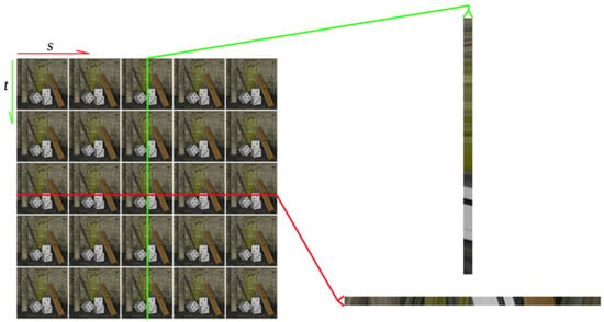
Figure 2.
The epipolar plane images. s and t denote the horizontal and vertical position within the multiple view image sets. With fixed t and spatial position y (which is inferred by the red line), we can get a slice representing the shift of a horizontal line from different views. We call this the horizontal epipolar plane image (EPI). The green line infers the vertical EPI.
2. Background and Related Work
The plenoptic camera has a micro-lens array lying in front of the sensor [2,5,6]. The image captured by the sensor can be broken up with the micro-lens array. Therefore, the sensor gathers light from different sources and directions, which is so-called Light-field photography.
There are some benefits of light fields compared to images captured by traditional cameras. First, users can refocus the picture after capturing. Second, a set of multiple-view images can be synthesized from a light field image which was captured in one single snapshot. Those multiple-view images, with different shifts in one snapshot, can construct the disparity in a nearly continuous space. These views are called as epipolar plane images (EPIs) [7]. Each corresponding pixel in the scene can be projected into a slope line in EPIs because of a dense sampling. The EPIs provide more information and robustness for depth estimation of the scene.
There hasn’t been much published work on depth estimation from light fields. Bishop and Favaro [8] first propose an analysis of aliasing in views captured by a plenoptic camera and a method to reduce the aliasing via space-varying filtering in the captured light field. In their later publication [9], they propose a method for full-resolution depth estimation by analyzing the correspondences in the sub-image .
An approach based on epipolar plane images (EPIs) is most popular recently. As mentioned in the previous section, the slope of line segments indicates disparity of the corresponding pixel. Therefore, depths can be found more easily if we can detect the slope of the line segments. Wanner et al. [10,11,12,13] propose an estimation by analyzing the local structure of the all-in-focus EPIs constructed by their novel method using the structure tensor, which is known to yield robust and accurate results for orientation. However, due to the local nature of the involved derivative filters, this method is able to recover disparities between two pixels, which implies small baselines between the cameras. Thus the depth analysis method severely restricts the possible camera setup parameters. Diebold and Goldluecke [14] improve Wanners’ method by applying refocusing on EPIs to eliminate lines with slope beyond the ability of tensor analyzing. Ng [6] demonstrates how to sharpen the EPIs to achieve refocusing.
Tao [15] proposed a similar approach to estimate depth from light fields. EPIs that have different slope value, that is, refocused in various depths, estimate depth from defocus and correspondence separately, and find the optimal solution by applying Markov Random Fields (MRF) optimization. However, because of relying on the slope of EPIs and a simple algorithm for defocus and correspondence, objects that are too far from the main lens focus plane will have an inaccurate estimation. Despite the poor performance, their method is the first to estimate depth from Lytro light field images.
Another approach based on EPIs is proposed by Kim et al. [16]. Unlike others’ works, which take images captured by light field cameras as the input, their method is designed to handle images with high resolution and dense angular-spatial resolution that are taken by a digital single-lens reflex camera. They claim to have the capability for parallel programming. They also propose a fine-to-coarse approach to achieve optimization for estimated depth. However, the result somehow depends on the quality of input images, that is, the correctness of estimation relies on how much information the input images can provide. For inputs that have poor quality, for example Lytro light field images with noise and blur, the performance of their method will be limited.
Since the product’s birth just a few years ago, light field cameras are still unpopular for consumers. Though Raytrix [3] has the ability to capture images with high quality, its high price and hardware requirement was unfriendly to consumers. Also, users have to connect Raytrix to a computer when they want to take pictures, and this is inconvenient when taking outdoor natural scenes. Lytro [4], on the other hand, is relatively easy to get because of the lower price. However, the data format for Lytro images has not been made public officially. The only choice for the researcher to use Lytro images is to decode the light field picture file (.lfp file) through a third-party toolbox. Moreover, these tools usually require camera-dependent data to achieve image calibration because the layout of the micro-lens array does not perfectly align due to manufacturing defects. We have tried some of these tools and hoped to find the one that suits our work.
D.G. et al. [17] provide a toolbox written in Matlab for calibration. Acquired from an open-source LFP picture decoder python-lfp-reader [18], the sensor’s raw data are composed of subimages lying hexagonally because of the layout of Lytro’s micro-lens array. This tool converts hexagonally sampled data to an orthogonal grid, and uses a 15-parameter camera model for calibration. It includes a 4D intrinsic matrix and a distortion model. Therefore, it can relate pixels to rays in 3D space. Their tool also provides a method to achieve color correction and image rectification. Though it outperforms in color, the images synthesized by the tool have poor quality with low resolution.
Cho et al. [19] propose another method to achieve calibration and multiple-view images reconstruction, which is easier to use and is able to obtain images with higher quality compared to the work described above. The raw data from the camera sensor is decoded by Nirav Patel’s project lfptools [20]. This work requires users to take a series of white images to detect the center and offset of each micro-lens as the preparation for calibration. They also analyze and evaluate several interpolation techniques for pixel resampling, and show that direct interpolation in raw images for a hexagonal grid produces better results than first making a low-resolution regular grid image. Finally, they propose a dictionary learning based interpolation technique which demonstrates a higher quality image reconstruction. The output of their system is already all-in-focus, that is, all the objects in the scene are in the range of depth of field, which is a convenience for depth estimation. Though being weak in color saturation, we decide to use images reconstructed by this work because of higher resolution and quality.
3. Depth Estimation
Our method takes a set of 5 × 5 multiple-view images as the input and comprises three stages: confidence measure, adaptive window matching and refinement. The light field images are smoothed by an edge-aware filter as preprocessing and are constructed into a 4D function for representation. Each pixel is then assigned a confidence value. The confidence not only decides window size for matching but also is influential in the stage of refinement. Next, we estimate depth by adaptive window matching. After all the pixels in the light field are assigned an estimated depth value, we apply an energy minimization to eliminate outliers and achieve optimization as the final result.
There are several ways to represent light fields. One way is to consider it as a collection of pinhole views from multiple viewpoints parallel to the image plane. In this work, we adopt a 4D function to represent light field data, which is so-called two-plane parametrization. Letting be the angular parameter referring to different viewpoints and be the spatial parameter of the image plane within a single view, we define to represent intensity value of the ray passing through the view point and the image plane position . s represents the horizontal angular position and t denotes the vertical one. If we fix a horizontal line with constant in the image plane and a constant angular coordinate , we will get a 2D slice that can show the shift of each pixel across each view. This view is called epipolar plane image (EPI), which is a common data structure when it comes to image analysis and 3D reconstruction.
A point in 3D space is projected to a line segment on the EPI slice. This is because of the densely sampled baseline of the micro-lens array. The slope of the line segment is related to its depth. As a result, we can estimate the depth of pixels according to slope m by the following equation at the corresponding position:
where f is a constant value referring to the distance between the micro-lens plane and the focused plane, and d is the displacement between two adjacent views. Thus, we can get the depth Z.
In this paper, we call EPI with fixed and the horizontal EPI (i.e., the EPI visualizes disparities of the horizontal lines), and the one with fixed and the vertical EPI. Therefore, the slope of the line segments can be estimated from vertical EPIs as well. For notation, we use to represent the pixel at position in horizontal EPI, and to represent that at position in vertical EPI.
Before starting the estimation, we first introduce how we measure confidence at each pixel, that is, whether the local structure at a certain position is confident enough to apply the estimation. The main concept for our depth estimation is to detect the slope of the line segment. However, there may be ambiguous regions due to a similar color. In this case, the slope we obtain may not be correct as shown in Figure 3. A way to avoid this problem is to assign confidence to the pixel according to source images. If it is in the region with high divergence, the depth estimated will have higher possibility to be correct, and thus we assign higher confidence to it.

Figure 3.
In ambiguous regions, slope may be incorrectly estimated. The blue line indicates the right slope, has higher possibility to be correctly estimated due to higher confidence. However, the slope of the red line may be incorrectly estimated due to the homogeneous color.
In order to enhance robustness of our confidence measure, we must consider that there may be some quality shortage such as noise in the input images. Therefore, we first apply an edge-aware filter to smooth the input, hoping to reduce the effect from noise. Instead of applying edge detection, the method we use for confidence measure is a simple difference measure inspired by [16]. Defining the confidence at position from view point , the measure of it is:
where is a 1D horizontal window centered at position from view point and is the vertical one. In our work we choose the window size to be 9.
Source confidence also points out the difficulty in obtaining the right depth. In the main step of depth computation, considering the robustness of estimation, we find optimal slope by matching 1D windows with disparities corresponding to the slope among different views. The size of the window is determined by its confidence. For pixels with higher confidence, it is possible that the slope of a line segment can be detected correctly. In other words, the lower confidence a pixel has, the bigger window size is needed for estimating depth. We define several intervals of confidence corresponding to different sizes where the relationship looks like:
Roughly, we divide into four intervals based on the confidence value with 0.2, 0.5 and 0.8. Each range will nearly double its window size.
With this rule, we can save the computing time for pixels with high confidence and still be able to obtain estimation that is dependable. Another meaning for the adaptive size is that if the confidence is low, it is usually relatively distant from the boundaries and has homogeneous color in the 1D window. On the other hands, sharp edges usually bring high confidence. So we have no need to worry that details will be eliminated during matching.
In this part, we demonstrate the core algorithm for depth estimation. We first select a position from viewpoint for estimation, and then measure the possibility with a series of hypothetical depths, which correspond to the slope on EPIs, and hope to get the optimal one through the method.
As mentioned previously, a selected position usually can correspond to two EPI slices: one is horizontal EPI and the other is vertical EPI . The two EPI slices will both be used for computing. As with the EPI slices, we have the horizontal window defined as and the vertical one as , centering at position on and on , where the size of the window is decided by source confidence. Let’s define the union of two patches sampled at a chosen position as the reference patch. For a chosen position and a hypothetical disparity d, a set of patches can be sampled as:
where n corresponds to the number of views in the light field. Figure 4 visualizes equation 4 more precisely. The set is the union of patches sampled at a shifted position according to the disparity from different view points. You can also interpret that we are trying to find the optimal shear value of a parallelogram that covers the range with maximal color consistency.

Figure 4.
The two parallelograms represent window matching with different window size in their optimal shear value (i.e., hypothetical d). For convenience of visualizing, we only show the ones on the horizontal EPI, but it can be applied on the vertical EPI as well.
Next we define how to measure the correctness of the set R with hypothetical disparity d. Our main concept of estimation is that if the hypothetical depth is the closest to ground truth, the difference between the reference patch and sampled patches should be the lowest. The score for set R with disparity d can be obtained by summing up similarities of corresponding pixels from the reference patch and sampled patches:
where is actually the simplified representation of the union , and is the union for the reference patch. The similarity between the two unions is defined as:
We apply a bell-shaped kernel to measure the similarity of intensity values between the two pixels, which is the same as was used by [16]. We set the threshold to 20% of the maximum color difference. The variable x was the normalized color difference. Thus, the bandwidth parameter h was set to 0.2 in our experiment. The kernel can be replaced by other kinds of bell-shaped kernel, such as the Gaussian kernel, but the kernel we chose takes less time to compute. For each selected position, we compute scores for the whole range of admissible disparities. The disparity d with the highest score will be assigned to the estimated depth at that position.
Remember that in the ambiguous region, the estimation has a relatively lower possibility to be correct. In other words, it may happen that scores for several hypothetical disparities are similar due to the region of similar color being larger than the window size. Therefore, in addition to source confidence , we define another confidence to denote how good the estimation is. We call this the estimated confidence . This confidence is obtained by dividing the highest score by the average score, where . Considering the two kinds of confidence together becomes meaningful as it combines two complementary measures. The comparison is shown in Figure 5. For example, in the noisy region, source confidence may become high while estimated confidence remains unreliable. The two confidence measurements will be used in the stage of refinement demonstrated in the following section.
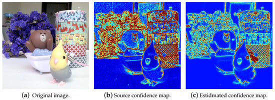
Figure 5.
Comparison between source confidence and estimated confidence. In the map, red color denotes higher confidence, and blue denotes lower confidence. In ambiguous regions, such as the floor or the background, source confidence becomes high because of noise, but the estimated confidence reduces the ambiguity.
4. Data Refinement
There may exist outliers which have survived the estimation process as shown in Figure 6. To eliminate the influences of these outliers, we apply an energy minimization algorithm. The goal of this step is to enhance consistency and smoothness for the region with similar colors, and meanwhile, preserve the estimation which is judged reliable. With the help of multiple-view input data, we also consider the consistency of the estimation at corresponding positions among multiple views.

Figure 6.
Temporary result from depth computing.
We first explain notations and their meaning used for our energy function. For simplification, we let v represent the viewpoint instead of , and i represent the position instead of . Therefore, the depth at position i from viewpoint v is then defined as . Our energy function can be separated into several parts:
In order to preserve estimations that are judged reliable, we define a local cost function which denotes how expensive it is to assign a depth value to the position i.
where denotes the depth value obtained from the previous stage, and is the product of source confidence and estimated confidence .
This term is defined for enhancing smoothness of depth values. Similar to the common smoothness energy term, the kernel is simply a second derivative kernel:
Depth values should satisfy consistency across multiple views. If a depth value is assigned to a particular position, the values on position belonging to the corresponding line segment should be consistent. We define representing the transferred position at view point according to depth value . To minimize the difference of sampled values, the energy term is defined as:
To avoid the occlusion case, the difference of the intensity cannot be over 20%. In the above equation, is a binary controller that will be 1 if , otherwise it will be 0.
Now we have all the elements for energy measurement. Letting be the union of multiple views depth sets, the quality of is evaluated as:
where , and are parameters controlling weights of each term. In general, all weights can be set equal to 1. To enhance the smoothing effect, is set to 6 in our experiment. Minimizing Equation (12) will give us , which is our ideal result. There are several ways to achieve energy minimization. We estimate the depth value from the neighbor that satisfies the Markov property. Thus, the cost function can be solved with the MRF optimization method. For implementation, we follow the framework introduced by Kappes et al. [21] which is a minimization method for Markov Random Fields. They have demonstrated different implementations for the MRF problem and have a good performance comparison among them. Also, they provide API with some optimization algorithms such as graph cuts [22,23,24] and their method is available at the website [25].
5. Experiment Results and Discussion
Honauer et al. [26] provides a dataset and evaluation methodology for depth estimation on 4D light fields. The data are diverse, including fine details, multiple planes, near and far objects. We have tested our algorithm with the dataset. The results are shown in Figure 7. The metrics from different datasets are shown in Table 1. Comparing our results with the ground truth, the results show that part of the error happened at the boundary that always has significant error. This error happens with incorrect window size.
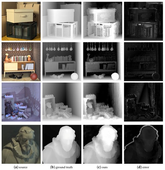
Figure 7.
compare the result to the ground truth. Reproduced from Reference [26] (CC BY-NC-SA 4.0).

Table 1.
Metrics from different datasets.
The adaptive window involves the boundary features to help the depth estimation and also includes the error. For a better estimate, we may need to decide the pixel belongs to the foreground or the background. However, that is not easy.
Datasets we use are taken by a first generation Lytro camera. As mentioned before, though users can view the captured images through Lytro’s official software, things we can do with the data are limited. Hence, we extract and decode the raw data from the sensor using the toolbox provided by Cho et al. [19]. Each dataset consists of multiple view images with a resolution of . In fact, the toolbox can extract at most images from a sensor’s raw data. However, the further from the central viewpoint an image is, the poorer quality it will have. As a result, we only choose central images for the experiment. Though the inputs are poor in color saturation and noisy due to hardware limitation, the quality is good enough to fit our framework. We prepare five datasets in this paper, and all of them are indoor scenes with obvious depth displacement.
Therefore, we compare our results with others’ for evaluation. We compare our work with Tao et al. [15] and Kim et al. [16]. Results of these comparisons are shown in Figure 8, Figure 9 and Figure 10. The method from Kim et al. is designed for inputs with high spatial and angular resolution. Because the code for the method is not provided, we implement it by ourselves. They claim that their algorithm works well on data with lower resolution such as those provided by [13]. However, when applied to low-quality inputs such as Lytro images, the method gets poor outputs. Tao’s method, on the other hand, is the first to estimate depth from Lytro images. Their system also handles the sensor’s raw data decoding, but the obtained resolution is limited to be about .
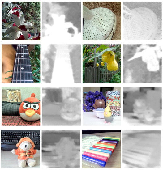
Figure 8.
Results from Tao’s method with their light field images and ours. The upper four images are data provided by Tao [15], and the others are ours. The performance is somehow a little bit different, but we didn’t make any change to their program.
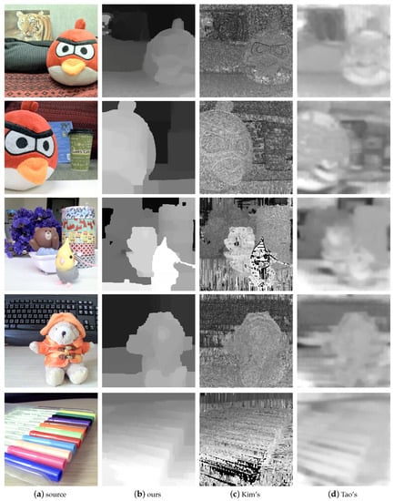
Figure 9.
Result for our method, Kim’s and Tao’s.
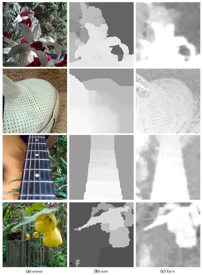
Figure 10.
Results from our method and Tao’s using Tao’s data [15]. Our results preserve objects’ edges and have less noise.
In the results from Tao’s method, boundaries are blurred, and it is hard to distinguish objects. This result is based on their MRF propagation process, which will smooth the whole image to achieve smoothness. Kim’s method, on the other hand, is vulnerable to the noisy quality of Lytro pictures. Another reason for the bad performance of Kim’s method may be the low number of views of the input dataset, where insufficient information reduces correctness of the estimation. In ours results, object contours are preserved and are consistently satisfactory. Though our method cannot obtain the correct estimation in some ambiguous regions, Kim’s and Tao’s methods also have this kind of problem.
Note that results from Tao’s method seem fine for their data. However, when we run their program with our input, the performance somehow isn’t as good as we expect. We suspect that the parameters we used that are different from Tao’s may be one source of the difference in the performance of Tao’s program between Tao’s input and our input.
Because our method relies on slope analysis to distinguish disparities, the scene used for the input must have obvious depth displacement. Also, since we take the color difference as the measure for estimation, it would be better if the difference between foreground and background is significant enough. Otherwise, occlusion may not be detected in the stage of adaptive window matching.
Another limitation of our method is that the MRF optimization algorithm will over-propagate the depth value in the concave region as shown in Figure 11. This phenomenon may happen after applying the optimization algorithm. In cases such as outdoor scenes with fine details, thin objects such as twigs may also be eliminated. Also, in some cases, our result shows an obvious depth gap rather than a continuous change in depth. The reason for this is that the shift of the images is too small (usually limited within pixels) for our algorithm to detect plenty of labels. Obviously, the current refinement process is not intelligent enough. In the result, we can see that the first stage is more noisy, but the refinement stage loses many details. The depth seems very flat. That is because of the smoothing term by the optimization algorithm. If the depth information was just used for segmentation, that will be okay. Otherwise, if the regularization can be steered by some local measures, maybe we can get a better result.
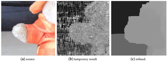
Figure 11.
Over-propagation happens in concave regions.
Right now, we did not involve any optimization for performance. The computation time for each scene is about twenty minutes. Both the first run and the refinement process need ten minutes. The complexity is linear with the number of images, the size of the picture, the size of matching windows and number of possible depth values.
6. Conclusions and Future Work
We present a method for depth estimation for Lytro images. Using third-party tools to decode the source .lfp file into a set of multiple-view images, we first measure the confidence by analyzing the structure of the origin pictures. We then apply adaptive window matching as the core of the depth computation. The adjustable size of the matching window enhances robustness and avoids incorrect estimation in the case of occlusion. For data refinement, we define an energy function to improve not only local smoothness but also global consistency. The data term of the energy function also considers the source confidence and estimated confidence, which we define as a measure of the probability that the estimate is correct. Energy minimization is achieved by following a framework of Markov Random Field optimization. Our results outperform current methods for handling depth estimation for light fields. That is because we first try to enhance the quality of source image sets by trying several tools and choosing the one that has the best performance. Moreover, the algorithm is designed to enhance robustness considering features of Lytro pictures. Though the computational cost is currently high, it can be greatly reduced because the estimation framework is able to undergo parallel processing on the GPU.
Acknowledgments
This work was supported in part by the National Science Council under the grants of MOST 105-2221-E-126-011.
Author Contributions
All of the authors contributed extensively to this work presented in the paper. Pei-Hsuan Lin has coordinated the work and participated in all section. Yung-Yu Chuang is as an advisor guiding the designing of image processing methods. Jeng-Sheng Yeh and FuChe WU provide suggestions to improve the algorithm and reorganize and revise the whole paper.
Conflicts of Interest
The authors declare no conflict of interest.
Abbreviations
The following abbreviations are used in this manuscript:
| EPI | Epipolar Plane Image |
| MRF | Markov Random Field |
References
- Adelson, E.; Bergen, J. The plenoptic function and the elements of early vision. Comput. Models Vis. Process. 1991, 1. Available online: http://faculty.cs.tamu.edu/jchai/CPSC641/elements91.pdf (accessed on 12 May 2017).
- Adelson, E.H.; Wang, J.Y.A. Single Lens Stereo with a Plenoptic Camera. IEEE Trans. Pattern Anal. Mach. Intell. 1992, 14, 99–106. [Google Scholar] [CrossRef]
- Raytrix. 3d Light Field Cameras. Available online: https://www.raytrix.de/produkte/ (accessed on 12 May 2017).
- Lytro. The Lytro ILLUM Camera. Available online: https://illum.lytro.com/illum (accessed on 12 May 2017).
- Lumsdaine, A.; Georgiev, T. The Focused Plenoptic Camera. In Proceedings of the 2009 IEEE International Conference on Computational Photography (ICCP), San Francisco, CA, USA, 16–17 April 2009; pp. 1–8. [Google Scholar]
- Ng, R.; Levoy, M.; Brédif, M.; Duval, G.; Horowitz, M.; Hanrahan, P. Light field photography with a hand-held plenoptic camera. Comput. Sci. Tech. Rep. CSTR 2005, 2, 1–11. [Google Scholar]
- Bolles, R.C.; Baker, H.H.; Marimont, D.H. Epipolarplane image analysis: An approach to determining structure from motion. Int. J. Comput. Vis. 1987, 1, 1–7. [Google Scholar] [CrossRef]
- Bishop, T.; Favaro, P. Plenoptic depth estimation from multiple aliased views. In Proceedings of the 2009 IEEE 12th International Conference on Computer Vision Workshops (ICCV Workshops), Kyoto, Japan, 27 September–4 October 2009; pp. 1622–1629. [Google Scholar]
- Bishop, T.; Favaro, P. Full-resolution depth map estimation from an aliased plenoptic light field. In Proceedings of the 10th Asian Conference on Computer Vision–Volume Part II, Queenstown, New Zealand, 8–12 November 2010; pp. 186–200. [Google Scholar]
- Wanner, S.; Fehr, J.; Jaehne, B. Generating EPI Representations of 4D Light Fields with a Single Lens Focused Plenoptic Camera. In Proceedings of the International Symposium on Visual Computing (ISVC 2011), Las Vegas, NV, USA, 26–28 September 2011. [Google Scholar]
- Wanner, S.; Goldluecke, B. Globally Consistent Depth Labeling of 4D Lightfields. In Proceedings of the IEEE Conference on Computer Vision and Pattern Recognition (CVPR), Providence, RI, USA, 16–21 June 2012. [Google Scholar]
- Goldluecke, B.; Wanner, S. The Variational Structure of Disparity and Regularization of 4D Light Fields. In Proceedings of the 2013 IEEE Conference on Computer Vision and Pattern Recognition (CVPR), Portland, OR, USA, 23–28 June 2013. [Google Scholar]
- Wanner, S.; Meister, S.; Goldluecke, B. Datasets and Benchmarks for Densely Sampled 4D Light Fields. In Proceedings of the 18th International Workshop on Vision, Modeling and Visualization (VMV 2013), Lugano, Switzerland, 11–13 September 2013. [Google Scholar]
- Diebold, M.; Goldluecke, B. Epipolar Plane Image Refocusing for Improved Depth Estimation and Occlusion Handling. In Proceedings of the 18th International Workshop on Vision, Modeling and Visualization (VMV 2013), Lugano, Switzerland, 11–13 September 2013. [Google Scholar]
- Tao, M.W.; Hadap, S.; Malik, J.; Ramamoorthi, R. Depth from Combining Defocus and Correspondence Using light-Field Cameras. In Proceedings of the 2013 International Conference on Computer Vision (ICCV), Sydney, Australia, 1–8 December 2013. [Google Scholar]
- Kim, C.; Zimmer, H.; Pritch, Y.; Sorkine-Hornung, A.; Gross, M. Scene Reconstruction from High Spatio-Angular Resolution Light Fields. ACM Trans. Graph. 2013, 32, 73:1–73:12. Available online: https://graphics.ethz.ch/~hzimmer/papers/kim-sig13/kim-sig13-paper-low.pdf (accessed on 12 May 2017). [CrossRef]
- Dansereau, D.; Pizarro, O.; Williams, S. Decoding, Calibration and Rectification for Lenselet-Based Plenoptic Cameras. In Proceedings of the 2013 IEEE Conference on Computer Vision and Pattern Recognition (CVPR), Portland, OR, USA, 23–28 June 2013; pp. 1027–1034. [Google Scholar]
- Python-lfp-reader. Python Library and Command-Line Scripts to Read Lytro LFP Files. Available online: http://code.behnam.es/python-lfp-reader/ (accessed on 12 May 2017).
- Cho, D.; Lee, M.; Kim, S.; Tai, Y.W. Modeling the Calibration Pipeline of the Lytro Camera for High Quality Light-Field Image Reconstruction. In Proceedings of the 2013 IEEE International Conference on Computer Vision (ICCV), Sydney, Australia, 1–8 December 2013; pp. 3280–3287. [Google Scholar]
- Nrpatel/lfptools. GitHub. Available online: https://github.com/nrpatel/lfptools (accessed on 12 May 2017).
- Kappes, J.H.; Andres, B.; Hamprecht, F.A.; Schnörr, C.; Nowozin, S.; Batra, D.; Kim, S.; Kausler, B.X.; Kröger, T.; Lellmann, J.; et al. A Comparative Study of Modern Inference Techniques for Structured Discrete Energy Minimization Problems. Int. J. Comput. Vision 2015, 115, 155–184. [Google Scholar] [CrossRef]
- Boykov, Y.; Veksler, O.; Zabih, R. Fast Approximate Energy Minimization via Graph Cuts. IEEE Trans. Pattern Anal. Mach. Intell. 2001, 23, 1222–1239. [Google Scholar] [CrossRef]
- Kolmogorov, V.; Zabih, R. What energy functions can be minimized via graph cuts. IEEE Trans. Pattern Anal. Mach. Intell. 2004, 26, 65–81. [Google Scholar] [CrossRef] [PubMed]
- Boykov, Y.; Kolmogorov, V. An Experimental Comparison of Min-Cut/Max-Flow Algorithms for Energy Minimization in Vision. IEEE Trans. Pattern Anal. Mach. Intell. 2004, 26, 1124–1137. [Google Scholar] [CrossRef] [PubMed]
- MRF (Markov Random Field). Available online: http://vision.middlebury.edu/MRF/ (accessed on 12 May 2017).
- Honauer, K.; Johannsen, O.; Kondermann, D.; Goldluecke, B. A Dataset and Evaluation Methodology for Depth Estimation on 4D Light Fields. In Proceedings of the Asian Conference on Computer Vision, Taipei, Taiwan, 20–26 November 2016; Springer: New York, NY, USA, 2016. [Google Scholar]
© 2017 by the authors. Licensee MDPI, Basel, Switzerland. This article is an open access article distributed under the terms and conditions of the Creative Commons Attribution (CC BY) license (http://creativecommons.org/licenses/by/4.0/).