
Segmentation of Non-Small Cell Lung Carcinomas: Introducing DRU-Net and Multi-Lens Distortion

 , , ,
, , ,
Abstract
1. Introduction
2. Materials and Methods
2.1. Cohorts
2.2. Ethical Aspects
2.3. Annotations and Dataset Preparation
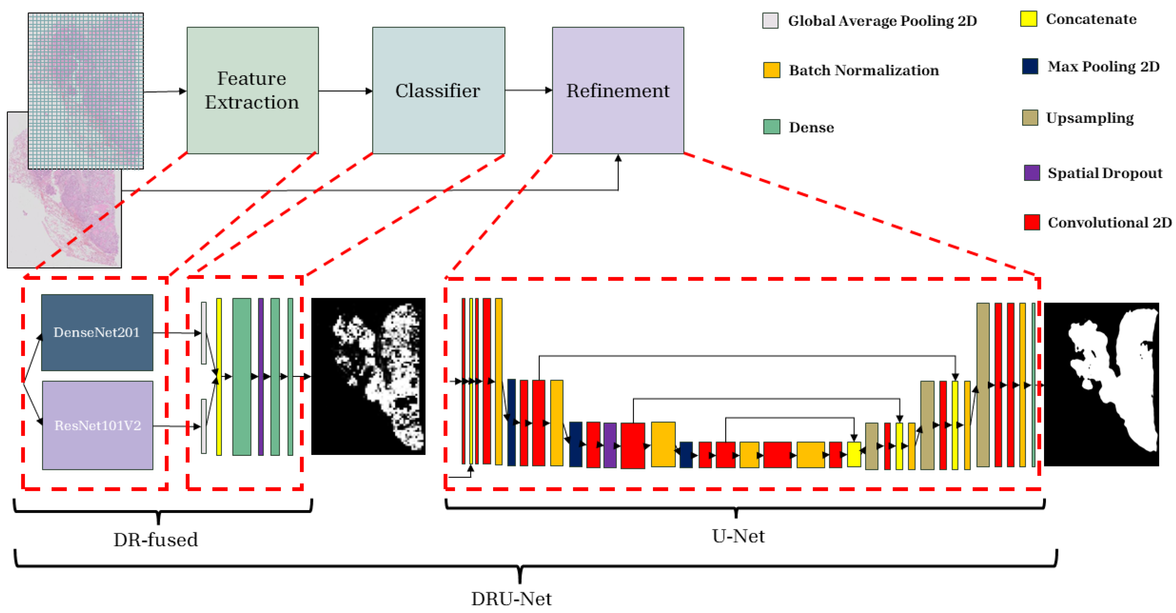
2.4. Proposed Method
2.4.1. Patch-Wise Classifier
2.4.2. Refinement Network
2.4.3. Data Augmentation
2.4.4. Multi-Lens Distortion Augmentation
| Algorithm 1 Multi-Lens Distortion (implementation-level pseudocode) |
| Require: , N ▹ number of lenses, , Ensure:
|
2.4.5. Model Training
2.4.6. Post-Processing
2.5. Implementation
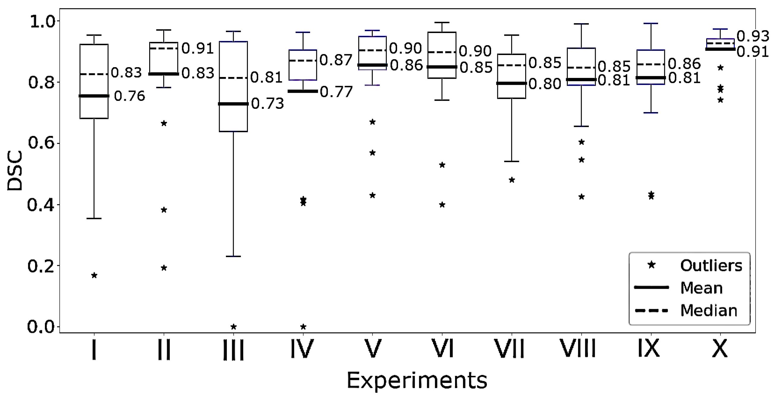
2.6. Experiments
2.7. Model Evaluation
2.7.1. Quantitative Model Assessment
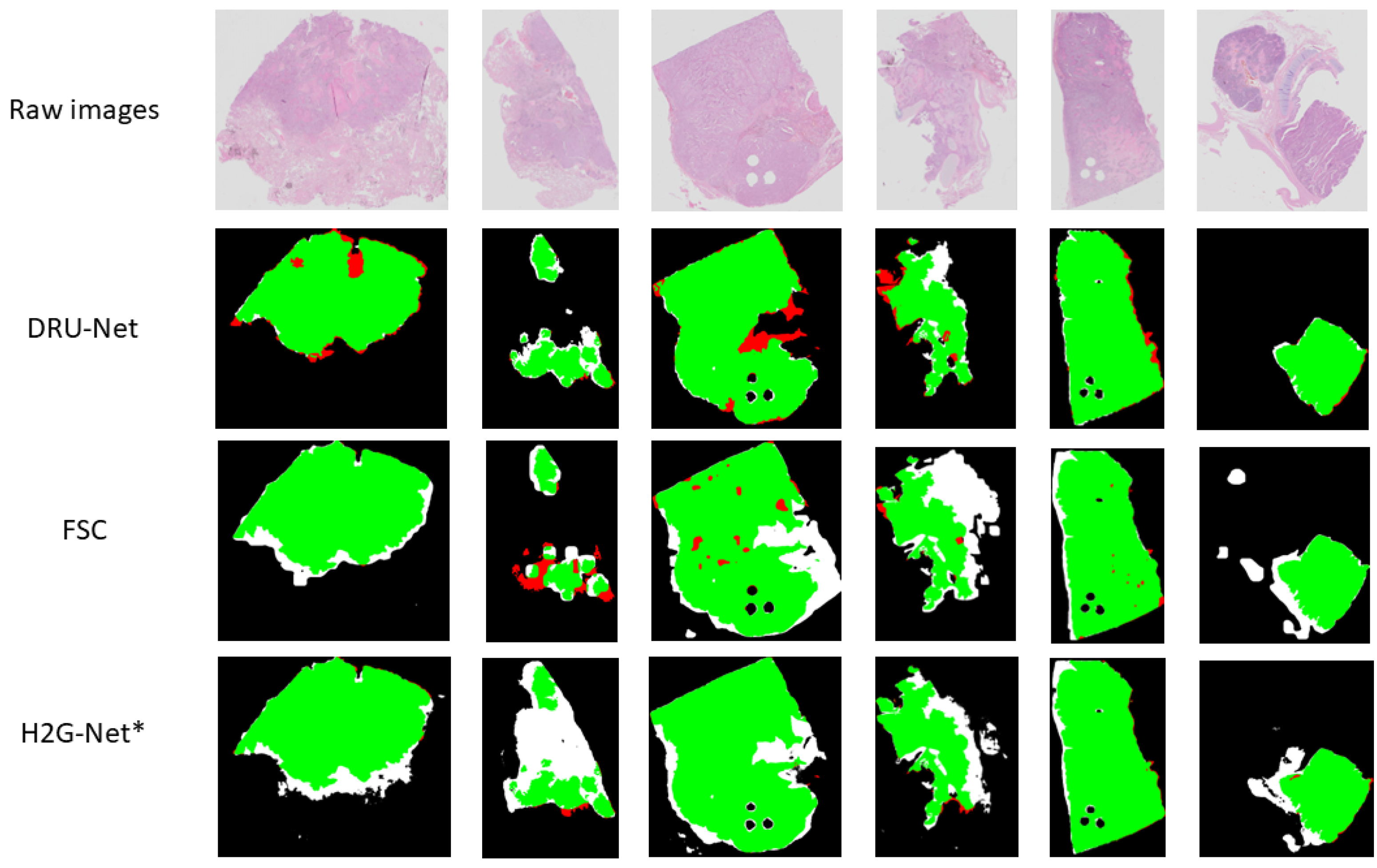
2.7.2. Qualitative Model Assessment
2.7.3. Saliency Maps
2.7.4. Computation of FLOPs and Parameters
3. Results
4. Discussion
5. Conclusions
Supplementary Materials
Author Contributions
Funding
Institutional Review Board Statement
Informed Consent Statement
Data Availability Statement
Acknowledgments
Conflicts of Interest
References
- Rami-Porta, R. Future perspectives on the TNM staging for lung cancer. Cancers 2021, 13, 1940. [Google Scholar] [CrossRef] [PubMed]
- Lim, C.; Tsao, M.; Le, L.; Shepherd, F.; Feld, R.; Burkes, R.; Liu, G.; Kamel-Reid, S.; Hwang, D.; Tanguay, J.; et al. Biomarker testing and time to treatment decision in patients with advanced nonsmall-cell lung cancer. Ann. Oncol. 2015, 26, 1415–1421. [Google Scholar] [CrossRef] [PubMed]
- Woodard, G.A.; Jones, K.D.; Jablons, D.M. Lung cancer staging and prognosis. In Lung Cancer Treatment and Research; Springer: Cham, Switzerland, 2016; pp. 47–75. [Google Scholar]
- Hanna, M.G.; Reuter, V.E.; Samboy, J.; England, C.; Corsale, L.; Fine, S.W.; Agaram, N.P.; Stamelos, E.; Yagi, Y.; Hameed, M.; et al. Implementation of digital pathology offers clinical and operational increase in efficiency and cost savings. Arch. Pathol. Lab. Med. 2019, 143, 1545–1555. [Google Scholar] [CrossRef] [PubMed]
- Bera, K.; Schalper, K.A.; Rimm, D.L.; Velcheti, V.; Madabhushi, A. Artificial intelligence in digital pathology—New tools for diagnosis and precision oncology. Nat. Rev. Clin. Oncol. 2019, 16, 703–715. [Google Scholar] [CrossRef]
- Sakamoto, T.; Furukawa, T.; Lami, K.; Pham, H.H.N.; Uegami, W.; Kuroda, K.; Kawai, M.; Sakanashi, H.; Cooper, L.A.D.; Bychkov, A.; et al. A narrative review of digital pathology and artificial intelligence: Focusing on lung cancer. Transl. Lung Cancer Res. 2020, 9, 2255–2276. [Google Scholar] [CrossRef]
- Niazi, M.K.K.; Parwani, A.V.; Gurcan, M.N. Digital pathology and artificial intelligence. Lancet Oncol. 2019, 20, e253–e261. [Google Scholar] [CrossRef]
- Kurc, T.; Bakas, S.; Ren, X.; Bagari, A.; Momeni, A.; Huang, Y.; Zhang, L.; Kumar, A.; Thibault, M.; Qi, Q.; et al. Segmentation and classification in digital pathology for glioma research: Challenges and deep learning approaches. Front. Neurosci. 2020, 14, 27. [Google Scholar] [CrossRef]
- Ho, D.J.; Yarlagadda, D.V.; D’Alfonso, T.M.; Hanna, M.G.; Grabenstetter, A.; Ntiamoah, P.; Brogi, E.; Tan, L.K.; Fuchs, T.J. Deep multi-magnification networks for multi-class breast cancer image segmentation. Comput. Med. Imaging Graph. 2021, 88, 101866. [Google Scholar] [CrossRef]
- Qaiser, T.; Tsang, Y.W.; Taniyama, D.; Sakamoto, N.; Nakane, K.; Epstein, D.; Rajpoot, N. Fast and accurate tumor segmentation of histology images using persistent homology and deep convolutional features. Med. Image Anal. 2019, 55, 1–14. [Google Scholar] [CrossRef]
- Zhao, T.; Fu, C.; Tie, M.; Sham, C.W.; Ma, H. RGSB-UNet: Hybrid Deep Learning Framework for Tumour Segmentation in Digital Pathology Images. Bioengineering 2023, 10, 957. [Google Scholar] [CrossRef]
- Viswanathan, V.S.; Toro, P.; Corredor, G.; Mukhopadhyay, S.; Madabhushi, A. The state of the art for artificial intelligence in lung digital pathology. J. Pathol. 2022, 257, 413–429. [Google Scholar] [CrossRef] [PubMed]
- Wang, S.; Yang, D.M.; Rong, R.; Zhan, X.; Fujimoto, J.; Liu, H.; Minna, J.; Wistuba, I.I.; Xie, Y.; Xiao, G. Artificial intelligence in lung cancer pathology image analysis. Cancers 2019, 11, 1673. [Google Scholar] [CrossRef] [PubMed]
- Davri, A.; Birbas, E.; Kanavos, T.; Ntritsos, G.; Giannakeas, N.; Tzallas, A.T.; Batistatou, A. Deep Learning for Lung Cancer Diagnosis, Prognosis and Prediction Using Histological and Cytological Images: A Systematic Review. Cancers 2023, 15, 3981. [Google Scholar] [CrossRef]
- Cheng, J.; Huang, K.; Xu, J. Computational pathology for precision diagnosis, treatment, and prognosis of cancer. Front. Med. 2023, 10, 1209666. [Google Scholar] [CrossRef]
- Ranftl, R.; Bochkovskiy, A.; Koltun, V. Vision transformers for dense prediction. In Proceedings of the IEEE/CVF International Conference on Computer Vision, Montreal, BC, Canada, 10–17 October 2021; pp. 12179–12188. [Google Scholar]
- Wang, W.; Dai, J.; Chen, Z.; Huang, Z.; Li, Z.; Zhu, X.; Hu, X.; Lu, T.; Lu, L.; Li, H.; et al. Internimage: Exploring large-scale vision foundation models with deformable convolutions. In Proceedings of the IEEE/CVF Conference on Computer Vision and Pattern Recognition, Nashville, TN, USA, 11–15 June 2023; pp. 14408–14419. [Google Scholar]
- Park, N.; Kim, S. How do vision transformers work? arXiv 2022, arXiv:2202.06709. [Google Scholar]
- Kassani, S.H.; Kassani, P.H.; Wesolowski, M.J.; Schneider, K.A.; Deters, R. Deep transfer learning based model for colorectal cancer histopathology segmentation: A comparative study of deep pre-trained models. Int. J. Med. Inform. 2022, 159, 104669. [Google Scholar] [CrossRef]
- Lin, H.; Chen, H.; Dou, Q.; Wang, L.; Qin, J.; Heng, P.A. ScanNet: A Fast and Dense Scanning Framework for Metastastic Breast Cancer Detection from Whole-Slide Image. In Proceedings of the 2018 IEEE Winter Conference on Applications of Computer Vision (WACV), Lake Tahoe, NV, USA, 12–15 March 2018; pp. 539–546. [Google Scholar] [CrossRef]
- Zeng, L.; Tang, H.; Wang, W.; Xie, M.; Ai, Z.; Chen, L.; Wu, Y. MAMC-Net: An effective deep learning framework for whole-slide image tumor segmentation. Multimed. Tools Appl. 2023, 82, 39349–39369. [Google Scholar] [CrossRef]
- Wang, L.; Pan, L.; Wang, H.; Liu, M.; Feng, Z.; Rong, P.; Chen, Z.; Peng, S. DHUnet: Dual-branch hierarchical global–local fusion network for whole slide image segmentation. Biomed. Signal Process. Control 2023, 85, 104976. [Google Scholar] [CrossRef]
- Pedersen, A.; Smistad, E.; Rise, T.V.; Dale, V.G.; Pettersen, H.S.; Nordmo, T.A.S.; Bouget, D.; Reinertsen, I.; Valla, M. H2G-Net: A multi-resolution refinement approach for segmentation of breast cancer region in gigapixel histopathological images. Front. Med. 2022, 9, 971873. [Google Scholar] [CrossRef]
- Albusayli, R.; Graham, D.; Pathmanathan, N.; Shaban, M.; Minhas, F.; Armes, J.E.; Rajpoot, N.M. Simple non-iterative clustering and CNNs for coarse segmentation of breast cancer whole-slide images. In Proceedings of the Medical Imaging 2021: Digital Pathology, Online, 15–20 February 2021; Volume 11603, pp. 100–108. [Google Scholar]
- Chelebian, E.; Avenel, C.; Ciompi, F.; Wählby, C. DEPICTER: Deep representation clustering for histology annotation. Comput. Biol. Med. 2024, 170, 108026. [Google Scholar] [CrossRef]
- Yan, J.; Chen, H.; Li, X.; Yao, J. Deep contrastive learning based tissue clustering for annotation-free histopathology image analysis. Comput. Med. Imaging Graph. 2022, 97, 102053. [Google Scholar] [CrossRef] [PubMed]
- Deuschel, J.; Firmbach, D.; Geppert, C.I.; Eckstein, M.; Hartmann, A.; Bruns, V.; Kuritcyn, P.; Dexl, J.; Hartmann, D.; Perrin, D.; et al. Multi-prototype few-shot learning in histopathology. In Proceedings of the IEEE/CVF International Conference on Computer Vision, Montreal, BC, Canada, 11–17 October 2021; pp. 620–628. [Google Scholar]
- Shakeri, F.; Boudiaf, M.; Mohammadi, S.; Sheth, I.; Havaei, M.; Ayed, I.B.; Kahou, S.E. FHIST: A benchmark for few-shot classification of histological images. arXiv 2022, arXiv:2206.00092. [Google Scholar]
- Titoriya, A.K.; Singh, M.P. Few-Shot Learning on Histopathology Image Classification. In Proceedings of the 2022 International Conference on Computational Science and Computational Intelligence (CSCI), Las Vegas, NV, USA, 14–16 December 2022; IEEE: Piscataway, NJ, USA, 2022; pp. 251–256. [Google Scholar]
- Liu, Z.; Lin, Y.; Cao, Y.; Hu, H.; Wei, Y.; Zhang, Z.; Lin, S.; Guo, B. Swin transformer: Hierarchical vision transformer using shifted windows. In Proceedings of the IEEE/CVF International Conference on Computer Vision, Montreal, BC, Canada, 11–17 October 2021; pp. 10012–10022. [Google Scholar]
- Liu, Z.; Mao, H.; Wu, C.Y.; Feichtenhofer, C.; Darrell, T.; Xie, S. A ConvNet for the 2020s. In Proceedings of the IEEE/CVF Conference on Computer Vision and Pattern Recognition, New Orleans, LA, USA, 18–24 June 2022; pp. 11976–11986. [Google Scholar]
- Krikid, F.; Rositi, H.; Vacavant, A. State-of-the-Art Deep Learning Methods for Microscopic Image Segmentation: Applications to Cells, Nuclei, and Tissues. J. Imaging 2024, 10, 311. [Google Scholar] [CrossRef] [PubMed]
- Greeley, C.; Holder, L.; Nilsson, E.E.; Skinner, M.K. Scalable deep learning artificial intelligence histopathology slide analysis and validation. Sci. Rep. 2024, 14, 26748. [Google Scholar] [CrossRef]
- Deng, R.; Cui, C.; Liu, Q.; Yao, T.; Remedios, L.W.; Bao, S.; Landman, B.A.; Wheless, L.E.; Coburn, L.A.; Wilson, K.T.; et al. Segment anything model (sam) for digital pathology: Assess zero-shot segmentation on whole slide imaging. In Proceedings of the IS&T International Symposium on Electronic Imaging, San Francisco, CA, USA, 2–6 February 2025; Volume 37, p. COIMG–132. [Google Scholar]
- Ma, J.; He, Y.; Li, F.; Han, L.; You, C.; Wang, B. Segment anything in medical images. Nat. Commun. 2024, 15, 654. [Google Scholar] [CrossRef]
- Huang, G.; Liu, Z.; Van Der Maaten, L.; Weinberger, K.Q. Densely Connected Convolutional Networks. In Proceedings of the IEEE Conference on Computer Vision and Pattern Recognition, Honolulu, HI, USA, 21–26 July 2017; pp. 4700–4708. [Google Scholar]
- He, K.; Zhang, X.; Ren, S.; Sun, J. Deep Residual Learning for Image Recognition. In Proceedings of the IEEE Conference on Computer Vision and Pattern Recognition, Las Vegas, NV, USA, 27–30 June 2016; pp. 770–778. [Google Scholar]
- Hatlen, P. Lung Cancer—Influence of Comorbidity on Incidence and Survival: The Nord-Trøndelag Health Study. Ph.D. Thesis, Norges Teknisk-Naturvitenskapelige Universitet, Det Medisinske Fakultet, Institutt for Sirkulasjon og Bildediagnostikk, Trondheim, Norway, 2014. [Google Scholar]
- Ramnefjell, M.; Aamelfot, C.; Helgeland, L.; Akslen, L.A. Vascular invasion is an adverse prognostic factor in resected non–small-cell lung cancer. Apmis 2017, 125, 197–206. [Google Scholar] [CrossRef]
- Hatlen, P.; Grønberg, B.H.; Langhammer, A.; Carlsen, S.M.; Amundsen, T. Prolonged survival in patients with lung cancer with diabetes mellitus. J. Thorac. Oncol. 2011, 6, 1810–1817. [Google Scholar] [CrossRef]
- Yoh Watanabe, M. TNM classification for lung cancer. Ann. Thorac. Cardiovasc. Surg. 2003, 9, 343–350. [Google Scholar]
- Travis, W. The 2015 WHO classification of lung tumors. Der Pathol. 2014, 35, 188. [Google Scholar] [CrossRef]
- Valla, M.; Vatten, L.J.; Engstrøm, M.J.; Haugen, O.A.; Akslen, L.A.; Bjørngaard, J.H.; Hagen, A.I.; Ytterhus, B.; Bofin, A.M.; Opdahl, S. Molecular subtypes of breast cancer: Long-term incidence trends and prognostic differences. Cancer Epidemiol. Biomark. Prev. 2016, 25, 1625–1634. [Google Scholar] [CrossRef]
- Deng, L. The MNIST Database of Handwritten Digit Images for Machine Learning Research. IEEE Signal Process. Mag. 2012, 29, 141–142. [Google Scholar] [CrossRef]
- Xiao, H.; Rasul, K.; Vollgraf, R. Fashion-MNIST: A Novel Image Dataset for Benchmarking Machine Learning Algorithms. arXiv 2017, arXiv:1708.07747. [Google Scholar]
- Krizhevsky, A. Learning Multiple Layers of Features from Tiny Images. Master’s Thesis, University of Tront, Toronto, ON, Canada, 2009. [Google Scholar]
- Bankhead, P.; Loughrey, M.B.; Fernández, J.A.; Dombrowski, Y.; McArt, D.G.; Dunne, P.D.; McQuaid, S.; Gray, R.T.; Murray, L.J.; Coleman, H.G.; et al. QuPath: Open source software for digital pathology image analysis. Sci. Rep. 2017, 7, 16878. [Google Scholar] [CrossRef]
- Deng, J.; Dong, W.; Socher, R.; Li, L.J.; Li, K.; Fei-Fei, L. ImageNet: A large-scale hierarchical image database. In Proceedings of the 2009 IEEE Conference on Computer Vision and Pattern Recognition, Miami, FL, USA, 20–25 June 2009; IEEE: Piscataway, NJ, USA, 2009; pp. 248–255. [Google Scholar]
- Abadi, M.; Agarwal, A.; Barham, P.; Brevdo, E.; Chen, Z.; Citro, C.; Corrado, G.S.; Davis, A.; Dean, J.; Devin, M.; et al. TensorFlow: Large-Scale Machine Learning on Heterogeneous Systems. 2015. Available online: https://www.tensorflow.org (accessed on 10 November 2023).
- Smistad, E.; Bozorgi, M.; Lindseth, F. FAST: Framework for heterogeneous medical image computing and visualization. Int. J. Comput. Assist. Radiol. Surg. 2015, 10, 1811–1822. [Google Scholar] [CrossRef]
- Smistad, E.; Østvik, A.; Pedersen, A. High performance neural network inference, streaming, and visualization of medical images using FAST. IEEE Access 2019, 7, 136310–136321. [Google Scholar] [CrossRef]
- Bradski, G. The OpenCV Library. Dr. Dobb’s J. Softw. Tools 2000, 120, 122–125. [Google Scholar]
- Clark, A. Pillow (PIL Fork) Documentation. 2015. Available online: https://buildmedia.readthedocs.org/media/pdf/pillow/latest/pillow.pdf (accessed on 10 November 2023).
- Harris, C.R.; Millman, K.J.; van der Walt, S.J.; Gommers, R.; Virtanen, P.; Cournapeau, D.; Wieser, E.; Taylor, J.; Berg, S.; Smith, N.J.; et al. Array programming with NumPy. Nature 2020, 585, 357–362. [Google Scholar] [CrossRef]
- Virtanen, P.; Gommers, R.; Oliphant, T.E.; Haberland, M.; Reddy, T.; Cournapeau, D.; Burovski, E.; Peterson, P.; Weckesser, W.; Bright, J.; et al. SciPy 1.0: Fundamental Algorithms for Scientific Computing in Python. Nat. Methods 2020, 17, 261–272. [Google Scholar] [CrossRef]
- Pedregosa, F.; Varoquaux, G.; Gramfort, A.; Michel, V.; Thirion, B.; Grisel, O.; Blondel, M.; Prettenhofer, P.; Weiss, R.; Dubourg, V.; et al. Scikit-learn: Machine Learning in Python. J. Mach. Learn. Res. 2011, 12, 2825–2830. [Google Scholar]
- Hunter, J.D. Matplotlib: A 2D graphics environment. Comput. Sci. Eng. 2007, 9, 90–95. [Google Scholar] [CrossRef]
- ONNX. Convert TensorFlow, Keras, Tensorflow.js and Tflite Models to ONNX. 2024. Available online: https://github.com/onnx/tensorflow-onnx (accessed on 10 November 2023).
- Pedersen, A.; Valla, M.; Bofin, A.M.; De Frutos, J.P.; Reinertsen, I.; Smistad, E. FastPathology: An open-source platform for deep learning-based research and decision support in digital pathology. IEEE Access 2021, 9, 58216–58229. [Google Scholar] [CrossRef]
- Sandler, M.; Howard, A.; Zhu, M.; Zhmoginov, A.; Chen, L.C. MobileNetV2: Inverted Residuals and Linear Bottlenecks. In Proceedings of the IEEE Conference on Computer Vision and Pattern Recognition, Salt Lake City, UT, USA, 18–23 June 2018; pp. 4510–4520. [Google Scholar]
- Goutte, C.; Gaussier, E. A probabilistic interpretation of precision, recall and F-score, with implication for evaluation. In Advances in Information Retrieval, Proceedings of the 27th European Conference on Information Retrieval, Santiago de Compostela, Spain, 21–23 March 2005; Springer: Berlin/Heidelberg, Germany, 2005; pp. 345–359. [Google Scholar]
- Kim, H.; Monroe, J.I.; Lo, S.; Yao, M.; Harari, P.M.; Machtay, M.; Sohn, J.W. Quantitative evaluation of image segmentation incorporating medical consideration functions. Med. Phys. 2015, 42, 3013–3023. [Google Scholar] [CrossRef] [PubMed]
- Patro, B.N.; Lunayach, M.; Patel, S.; Namboodiri, V.P. U-CAM: Visual Explanation using Uncertainty based Class Activation Maps. In Proceedings of the IEEE/CVF International Conference on Computer Vision, Seoul, Republic of Korea, 27 October–2 November 2019; pp. 7444–7453. [Google Scholar]
- Simonyan, K.; Vedaldi, A.; Zisserman, A. Deep inside convolutional networks: Visualising image classification models and saliency maps. arXiv 2013, arXiv:1312.6034. [Google Scholar]
- Zeiler, M.D.; Fergus, R. Visualizing and understanding convolutional networks. In Computer Vision–ECCV 2014, Proceedings of the 13th European Conference, Zurich, Switzerland, 6–12 September 2014; Proceedings, Part I 13; Springer: Berlin/Heidelberg, Germany, 2014; pp. 818–833. [Google Scholar]
- Sundararajan, M.; Taly, A.; Yan, Q. Axiomatic attribution for deep networks. In Proceedings of the International Conference on Machine Learning, Sydney, Australia, 6–11 August 2017; pp. 3319–3328. [Google Scholar]
- Simonyan, K.; Zisserman, A. Very Deep Convolutional Networks for Large-Scale Image Recognition. arXiv 2014, arXiv:1409.1556. [Google Scholar]
- Tan, M.; Le, Q. EfficientNetV2: Smaller Models and Faster Training. In Proceedings of the International Conference on Machine Learning, Virtual, 18–24 July 2021; pp. 10096–10106. [Google Scholar]
- Szegedy, C.; Vanhoucke, V.; Ioffe, S.; Shlens, J.; Wojna, Z. Rethinking the Inception Architecture for Computer Vision. In Proceedings of the IEEE Conference on Computer Vision and Pattern Recognition, Las Vegas, NV, USA, 27–30 June 2016; pp. 2818–2826. [Google Scholar]
- Gai, L.; Xing, M.; Chen, W.; Zhang, Y.; Qiao, X. Comparing CNN-based and transformer-based models for identifying lung cancer: Which is more effective? Multimed. Tools Appl. 2024, 83, 59253–59269. [Google Scholar] [CrossRef]
- Sangeetha, S.; Mathivanan, S.K.; Muthukumaran, V.; Cho, J.; Easwaramoorthy, S.V. An Empirical Analysis of Transformer-Based and Convolutional Neural Network Approaches for Early Detection and Diagnosis of Cancer Using Multimodal Imaging and Genomic Data. IEEE Access 2025, 13, 6120–6145. [Google Scholar] [CrossRef]
- Lakshmanan, B.; Anand, S.; Jenitha, T. Stain removal through color normalization of haematoxylin and eosin images: A review. Proc. J. Phys. Conf. Ser. 2019, 1362, 012108. [Google Scholar] [CrossRef]
- Tellez, D.; Litjens, G.; Bándi, P.; Bulten, W.; Bokhorst, J.M.; Ciompi, F.; Van Der Laak, J. Quantifying the effects of data augmentation and stain color normalization in convolutional neural networks for computational pathology. Med. Image Anal. 2019, 58, 101544. [Google Scholar] [CrossRef]
- Cao, H.; Wang, Y.; Chen, J.; Jiang, D.; Zhang, X.; Tian, Q.; Wang, M. Swin-unet: Unet-like pure transformer for medical image segmentation. In Computer Vision—ECCV 2022 Workshops, Proceedings of the European Conference on Computer Vision, Tel Aviv, Israel, 23–27 October 2022; Springer: Cham, Switzerland, 2022; pp. 205–218. [Google Scholar]
- Dosovitskiy, A.; Beyer, L.; Kolesnikov, A.; Weissenborn, D.; Zhai, X.; Unterthiner, T.; Dehghani, M.; Minderer, M.; Heigold, G.; Gelly, S.; et al. An image is worth 16x16 words: Transformers for image recognition at scale. arXiv 2020, arXiv:2010.11929. [Google Scholar]
- Lin, T.Y.; Goyal, P.; Girshick, R.; He, K.; Dollár, P. Focal loss for dense object detection. In Proceedings of the IEEE International Conference on Computer Vision, Venice, Italy, 22–29 October 2017; pp. 2980–2988. [Google Scholar]
- Menon, A.; Singh, P.; Vinod, P.; Jawahar, C. Exploring Histological Similarities Across Cancers from a Deep Learning Perspective. Front. Oncol. 2022, 12, 842759. [Google Scholar] [CrossRef]
- Kashima, J.; Kitadai, R.; Okuma, Y. Molecular and Morphological Profiling of Lung Cancer: A Foundation for “Next-Generation" Pathologists and Oncologists. Cancers 2019, 11, 599. [Google Scholar] [CrossRef] [PubMed]
- Petersen, I. The morphological and molecular diagnosis of lung cancer. Dtsch. Ärztebl. Int. 2011, 108, 525–531. [Google Scholar] [CrossRef] [PubMed]
- Inamura, K. Lung cancer: Understanding its molecular pathology and the 2015 WHO classification. Front. Oncol. 2017, 7, 193. [Google Scholar] [CrossRef] [PubMed]
- Zhao, S.; Chen, D.P.; Fu, T.; Yang, J.C.; Ma, D.; Zhu, X.Z.; Wang, X.X.; Jiao, Y.P.; Jin, X.; Xiao, Y.; et al. Single-cell morphological and topological atlas reveals the ecosystem diversity of human breast cancer. Nat. Commun. 2023, 14, 6796. [Google Scholar] [CrossRef]
- Binder, A.; Bockmayr, M.; Hägele, M.; Wienert, S.; Heim, D.; Hellweg, K.; Ishii, M.; Stenzinger, A.; Hocke, A.; Denkert, C.; et al. Morphological and molecular breast cancer profiling through explainable machine learning. Nat. Mach. Intell. 2021, 3, 355–366. [Google Scholar] [CrossRef]
- Tan, P.H.; Ellis, I.; Allison, K.; Brogi, E.; Fox, S.B.; Lakhani, S.; Lazar, A.J.; Morris, E.A.; Sahin, A.; Salgado, R.; et al. The 2019 WHO classification of tumours of the breast. Histopathology 2020, 77, 181–185. [Google Scholar] [CrossRef]
- Qi, Y.; Sun, H.; Liu, N.; Zhou, H. A Task-Aware Dual Similarity Network for Fine-Grained Few-Shot Learning. In PRICAI 2022: Trends in Artificial Intelligence, Proceedings of the Pacific Rim International Conference on Artificial Intelligence, Shanghai, China, 10–13 November 2022; Springer: Cham, Switzerland, 2022; pp. 606–618. [Google Scholar]
- Achanta, R.; Shaji, A.; Smith, K.; Lucchi, A.; Fua, P.; Süsstrunk, S. Slic Superpixels; Ecole Polytechnique F´edrale de Lausanne (EPFL): Lausanne, Switzerland, 2010. [Google Scholar]


| Histological Subtype | NLCB (n,%) | HULC—Train (n, %) | HULC—Test (n, %) |
|---|---|---|---|
| AC | 16 (38.1%) | 38 (49.4%) | 7 (35.0%) |
| SCC | 15 (35.7%) | 32 (41.6%) | 10 (50.0%) |
| Other NSCC | 11 (26.2%) | 7 (9.1%) | 3 (15.0%) |
| Total number of WSIs | 42 | 77 | 20 |
| Models | Modifications | Training Dataset (s) | |
|---|---|---|---|
| (I) | H2G-Net | — | — |
| (II) | H2G-Net | Fine-tuned PWC | HULC Cohort |
| (III) | H2G-Net | Fine-tuned U-Net | HULC Cohort |
| (IV) | H2G-Net | Fine-tuned PWC and original U-Net | HULC Cohort |
| (V) | DRU-Net | — | HULC Cohort |
| (VI) | H2G-Net | Fine-tuned PWC | NLCB |
| (VII) | H2G-Net | Fine-tuned PWC and U-Net | PWC trained on NLCB, U-Net trained on HULC Cohort |
| (VIII) | FSC | — | NLCB |
| (IX) | MSC | — | NLCB |
| (X) | DRU-Net | — | PWC trained on NLCB, U-Net trained on HULC Cohort |
| 0 | 1 | 2 | 3 | 4 | 5 |
|---|---|---|---|---|---|
| No tumor tissue in image or segmentation, or image not suitable for analysis | Completely wrong segmentation of tumor, tumor tissue not segmented | A large part of the tumor is not segmented | Most of the tumor is correctly segmented, but some false positive or false negative areas | Most of the tumor is correctly segmented, only sparse false positive or false negative areas | The whole or almost the whole tumor correctly segmented |
| F1-Score | ||||
|---|---|---|---|---|
| Model | Dataset | W/O Aug | W/ Aug | p-Value |
| DenseNet121 | MNIST | 0.9893 | 0.9894 | 0.2311 |
| DenseNet121 | Fashion-MNIST | 0.9043 | 0.9208 | <0.001 |
| DenseNet121 | CIFAR-10 | 0.8086 | 0.8235 | <0.001 |
| DenseNet121 | CIFAR-100 | 0.5199 | 0.5581 | 0.0502 |
| H2G-Net | NLCB | 0.8299 | 0.8341 | 0.0701 |
| DRU-Net | NLCB | 0.8868 | 0.9025 | 0.0241 |
| Architecture | F1-Score | Precision | Recall |
|---|---|---|---|
| VGG19 [67] | 0.87 | 0.86 | 0.87 |
| ResNet101V2 [37] | 0.89 | 0.89 | 0.89 |
| MobileNetV2 [60] | 0.86 | 0.86 | 0.86 |
| EfficientNetV2 [68] | 0.89 | 0.89 | 0.89 |
| InceptionV3 [69] | 0.90 | 0.89 | 0.91 |
| DenseNet201 [36] | 0.91 | 0.91 | 0.91 |
| Proposed DR-Fused | 0.94 | 0.94 | 0.93 |
| Architecture | FLOPs (M) | Params (M) | ΔFLOPs (%) | ΔParams (%) |
|---|---|---|---|---|
| DR-Fused | 11,105.27 | 13.18 | 1712.42 | 483.02 |
| VGG19 [67] | 39,276.93 | 139.58 | 6310.14 | 6074.55 |
| ResNet101V2 [37] | 14,430.04 | 42.63 | 2255.04 | 1785.86 |
| MobileNetV2 [60] | 612.73 | 2.26 | 0.00 | 0.00 |
| EfficientNetV2 [68] | 1455.32 | 5.92 | 137.51 | 161.97 |
| InceptionV3 [69] | 5693.36 | 21.81 | 829.18 | 864.67 |
| DenseNet201 [36] | 8631.68 | 18.33 | 1308.72 | 710.68 |
Disclaimer/Publisher’s Note: The statements, opinions and data contained in all publications are solely those of the individual author(s) and contributor(s) and not of MDPI and/or the editor(s). MDPI and/or the editor(s) disclaim responsibility for any injury to people or property resulting from any ideas, methods, instructions or products referred to in the content. |
© 2025 by the authors. Licensee MDPI, Basel, Switzerland. This article is an open access article distributed under the terms and conditions of the Creative Commons Attribution (CC BY) license (https://creativecommons.org/licenses/by/4.0/).
Share and Cite
Oskouei, S.; Valla, M.; Pedersen, A.; Smistad, E.; Dale, V.G.; Høibø, M.; Wahl, S.G.F.; Haugum, M.D.; Langø, T.; Ramnefjell, M.P.; et al. Segmentation of Non-Small Cell Lung Carcinomas: Introducing DRU-Net and Multi-Lens Distortion. J. Imaging 2025, 11, 166. https://doi.org/10.3390/jimaging11050166
Oskouei S, Valla M, Pedersen A, Smistad E, Dale VG, Høibø M, Wahl SGF, Haugum MD, Langø T, Ramnefjell MP, et al. Segmentation of Non-Small Cell Lung Carcinomas: Introducing DRU-Net and Multi-Lens Distortion. Journal of Imaging. 2025; 11(5):166. https://doi.org/10.3390/jimaging11050166
Chicago/Turabian StyleOskouei, Soroush, Marit Valla, André Pedersen, Erik Smistad, Vibeke Grotnes Dale, Maren Høibø, Sissel Gyrid Freim Wahl, Mats Dehli Haugum, Thomas Langø, Maria Paula Ramnefjell, and et al. 2025. "Segmentation of Non-Small Cell Lung Carcinomas: Introducing DRU-Net and Multi-Lens Distortion" Journal of Imaging 11, no. 5: 166. https://doi.org/10.3390/jimaging11050166
APA StyleOskouei, S., Valla, M., Pedersen, A., Smistad, E., Dale, V. G., Høibø, M., Wahl, S. G. F., Haugum, M. D., Langø, T., Ramnefjell, M. P., Akslen, L. A., Kiss, G., & Sorger, H. (2025). Segmentation of Non-Small Cell Lung Carcinomas: Introducing DRU-Net and Multi-Lens Distortion. Journal of Imaging, 11(5), 166. https://doi.org/10.3390/jimaging11050166