
Real-Time Far-Field BCSDF Filtering


Abstract
1. Introduction
- A joint filtering framework for BCSDFs and tangent maps, enabling real-time level-of-detail (LoD) rendering of BCSDFs.
- An analytical effective BCSDF formulation based on the von Mises–Fisher (vMF) distribution, preserving intrinsic optical scattering properties while admitting closed-form convolution with TDFs.
- A novel Clustered Control Variates (CCV) integration scheme for efficiently approximating the convolution of the TT lobe.
2. Related Work
3. Method
3.1. Background
3.2. BCSDF Filtering via vMFs
3.3. Closed Form of vMF Convolution
3.4. Implementation
4. Result
5. Conclusions
6. Future Work
Author Contributions
Funding
Institutional Review Board Statement
Informed Consent Statement
Data Availability Statement
Conflicts of Interest
Abbreviations
| BCSDF | Bidirectional Curve Scattering Distribution Function |
| TDF | Tangent Distribution Function |
| vMF | von Mises–Fisher Distribution |
| CCV | Clustered Control Variates |
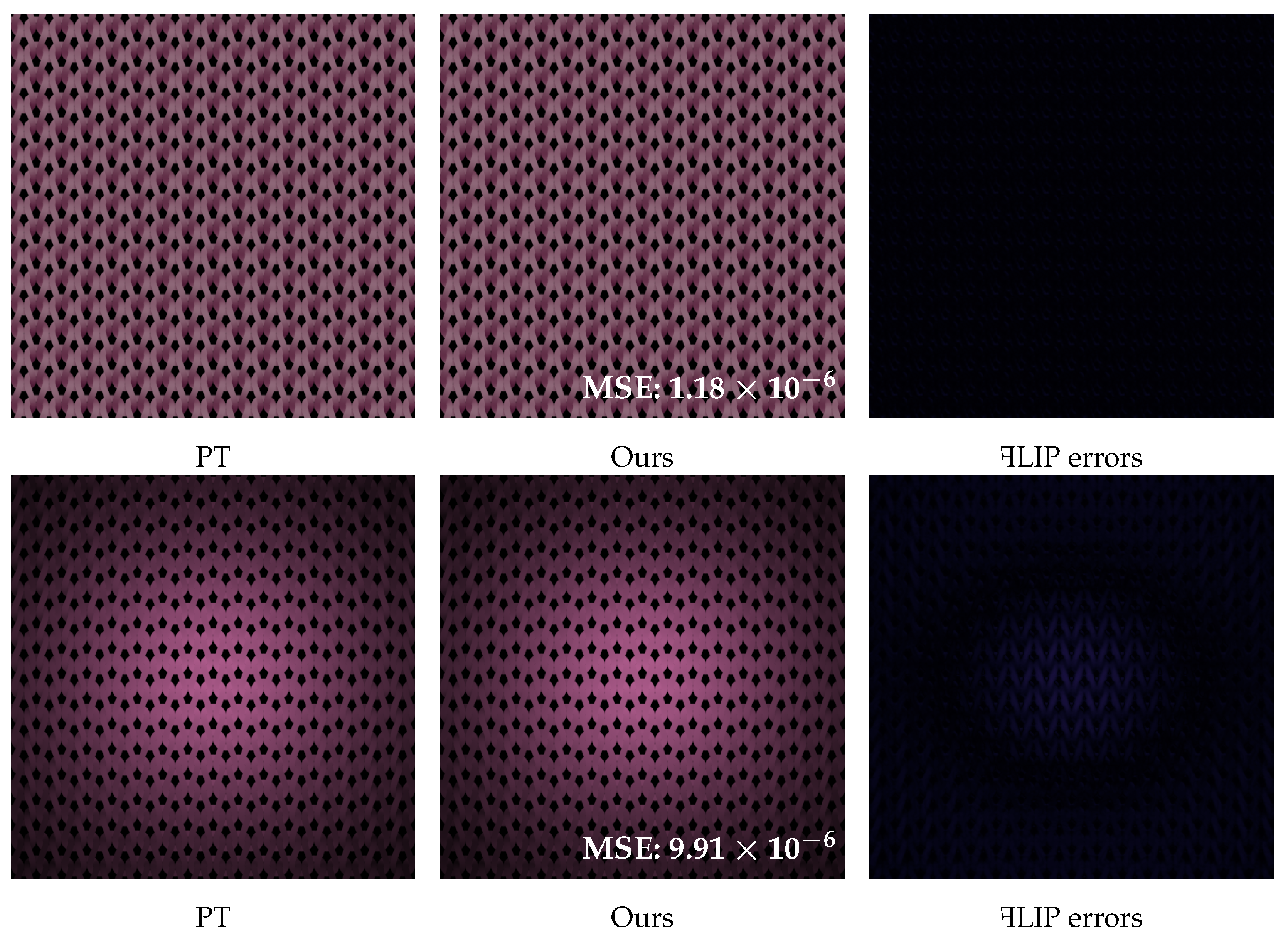
| MSE | Mean squared error |
References
- Zhu, J.; Jarabo, A.; Aliaga, C.; Yan, L.Q.; Chiang, M.J.Y. A realistic surface-based cloth rendering model. In Proceedings of the ACM SIGGRAPH 2023 Conference Proceedings, Los Angeles, CA, USA, 6–10 August 2023; pp. 1–9. [Google Scholar]
- Zhu, J.; Hery, C.; Bode, L.; Aliaga, C.; Jarabo, A.; Yan, L.Q.; Chiang, M.J.Y. A Realistic Multi-scale Surface-based Cloth Appearance Model. In Proceedings of the ACM SIGGRAPH 2024 Conference, Denver, CO, USA, 27 July–1 August 2024; pp. 1–10. [Google Scholar]
- Ramamoorthi, R.; Hanrahan, P. A signal-processing framework for inverse rendering. In Proceedings of the 28th Annual Conference on Computer Graphics and Interactive Techniques, Los Angeles, CA, USA, 12–17 August 2001; pp. 117–128. [Google Scholar]
- Xu, C.; Wang, R.; Zhao, S.; Bao, H. Real-Time Linear BRDF MIP-Mapping. Comput. Graph. Forum 2017, 36, 27–34. [Google Scholar] [CrossRef]
- Olano, c.; Baker, D. Lean mapping. In Proceedings of the 2010 ACM SIGGRAPH Symposium on Interactive 3D Graphics and Games, Washington, DC, USA, 19–21 February 2010; pp. 181–188. [Google Scholar]
- Han, C.; Sun, B.; Ramamoorthi, R.; Grinspun, E. Frequency domain normal map filtering. In ACM SIGGRAPH 2007 Papers; Association for Computing Machinery: New York, NY, USA, 2007; p. 28-es. [Google Scholar]
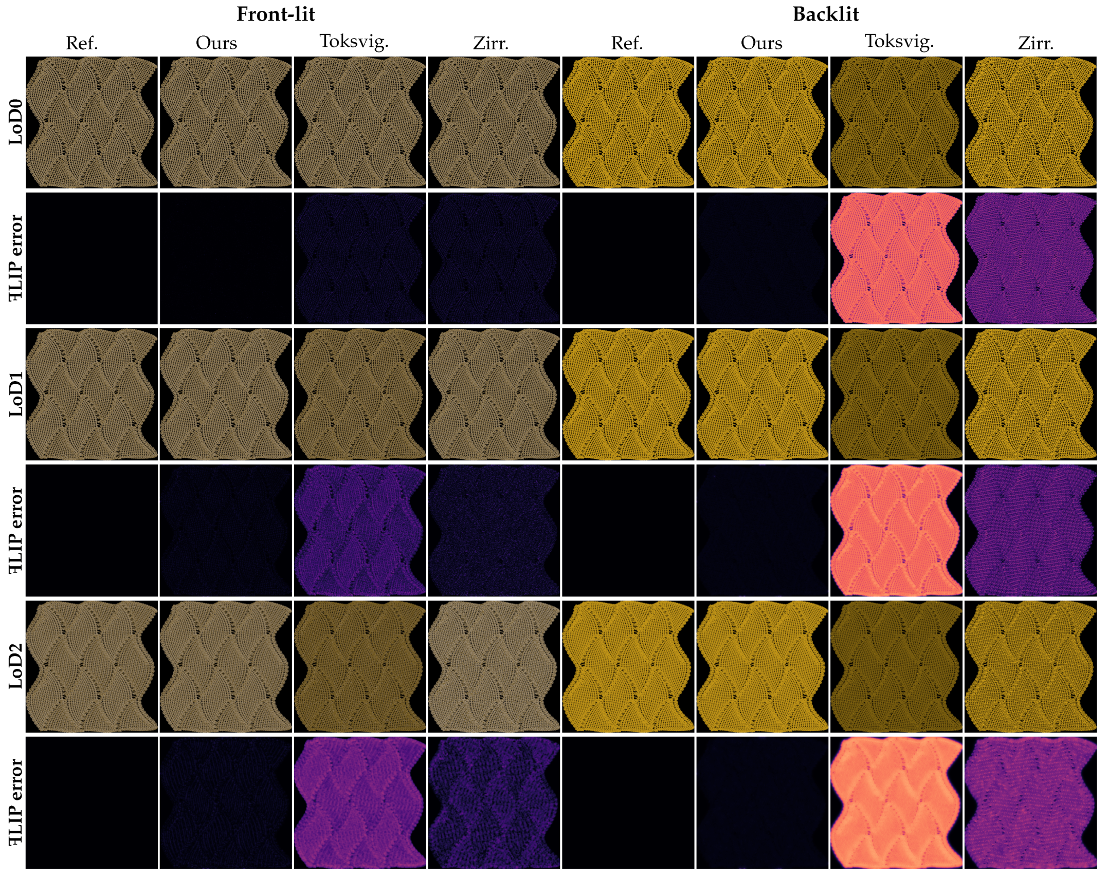
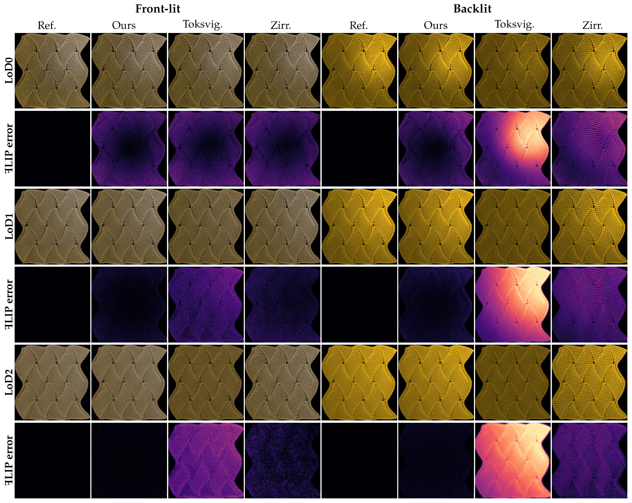
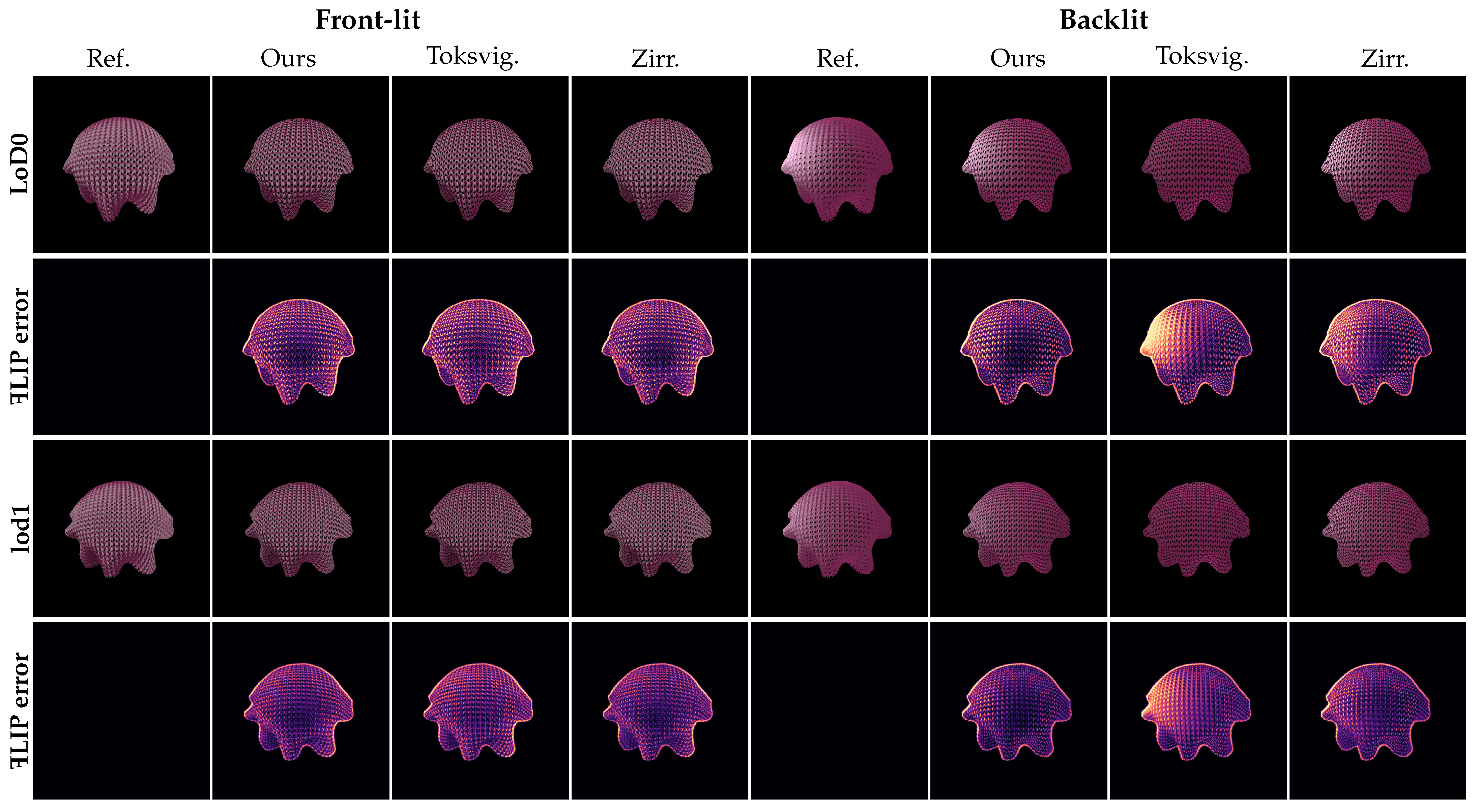
- Toksvig, M. Mipmapping normal maps. J. Graph. Tools 2005, 10, 65–71. [Google Scholar] [CrossRef]
- Zirr, T.; Kaplanyan, A.S. Real-time rendering of procedural multiscale materials. In Proceedings of the 20th ACM SIGGRAPH Symposium on Interactive 3D Graphics and Games, Redmond, WA, USA, 26–28 February 2016; pp. 139–148. [Google Scholar]
- Marschner, S.R.; Jensen, H.W.; Cammarano, M.; Worley, S.; Hanrahan, P. Light scattering from human hair fibers. ACM Trans. Graph. (TOG) 2003, 22, 780–791. [Google Scholar] [CrossRef]
- d’Eon, E.; Francois, G.; Hill, M.; Letteri, J.; Aubry, J.M. An energy-conserving hair reflectance model. Comput. Graph. Forum 2011, 30, 1181–1187. [Google Scholar] [CrossRef]
- Chiang, M.J.Y.; Bitterli, B.; Tappan, C.; Burley, B. A Practical and Controllable Hair and Fur Model for Production Path Tracing. Comput. Graph. Forum 2016, 35, 275–283. [Google Scholar] [CrossRef]
- Zinke, A.; Yuksel, C.; Weber, A.; Keyser, J. Dual scattering approximation for fast multiple scattering in hair. In ACM SIGGRAPH 2008 Papers; Association for Computing Machinery: New York, NY, USA, 2008; pp. 1–10. [Google Scholar]
- Khungurn, P.; Schroeder, D.; Zhao, S.; Bala, K.; Marschner, S. Matching Real Fabrics with Micro-Appearance Models. ACM Trans. Graph. 2016, 35, 1. [Google Scholar] [CrossRef]
- Yan, L.Q.; Tseng, C.W.; Jensen, H.W.; Ramamoorthi, R. Physically-accurate fur reflectance: Modeling, measurement and rendering. ACM Trans. Graph. (TOG) 2015, 34, 185. [Google Scholar] [CrossRef]
- Yan, L.Q.; Sun, W.; Jensen, H.W.; Ramamoorthi, R. A BSSRDF model for efficient rendering of fur with global illumination. ACM Trans. Graph. (TOG) 2017, 36, 208. [Google Scholar] [CrossRef]
- Montazeri, Z.; Gammelmark, S.; Jensen, H.W.; Zhao, S. A Practical Ply-Based Appearance Modeling for Knitted Fabrics. arXiv 2021, arXiv:2105.02475. [Google Scholar]
- Montazeri, Z.; Gammelmark, S.B.; Zhao, S.; Jensen, H.W. A practical ply-based appearance model of woven fabrics. ACM Trans. Graph. (TOG) 2020, 39, 251. [Google Scholar] [CrossRef]
- Wu, K.; Yuksel, C. Real-time cloth rendering with fiber-level detail. IEEE Trans. Vis. Comput. Graph. 2017, 25, 1297–1308. [Google Scholar] [CrossRef] [PubMed]
- Chen, X.; Wang, L.; Wang, B. Real-time Neural Woven Fabric Rendering. In Proceedings of the ACM SIGGRAPH 2024 Conference, Denver, CO, USA, 27 July–1 August 2024; pp. 1–10. [Google Scholar]
- Xu, Z.; Montazeri, Z.; Wang, B.; Yan, L.Q. A Dynamic By-example BTF Synthesis Scheme. In Proceedings of the SIGGRAPH Asia 2024 Conference, Tokyo, Japan, 3–6 December 2024; pp. 1–10. [Google Scholar]
- Fournier, A. Normal Distribution Functions and Multiple Surfaces. In Proceedings of the Graphics Interface ’92 Workshop on Local Illumination, Vancouver, BC, Canada, 11 May 1992; pp. 45–52. [Google Scholar]
- Becker, B.G.; Max, N.L. Smooth transitions between bump rendering algorithms. In Proceedings of the 20th Annual Conference on Computer Graphics and Interactive Techniques, Anaheim, CA, USA, 2–6 August 1993; pp. 183–190. [Google Scholar]
- Dupuy, J.; Heitz, E.; Iehl, J.C.; Poulin, P.; Neyret, F.; Ostromoukhov, V. Linear efficient antialiased displacement and reflectance mapping. ACM Trans. Graph. (TOG) 2013, 32, 211. [Google Scholar] [CrossRef]
- Chermain, X.; Lucas, S.; Sauvage, B.; Dischler, J.M.; Dachsbacher, C. Real-time geometric glint anti-aliasing with normal map filtering. In Proceedings of the ACM on Computer Graphics and Interactive Techniques, Virtual, 9–13 August 2021; Volume 4, pp. 1–16. [Google Scholar]
- Bruneton, E.; Neyret, F. A survey of nonlinear prefiltering methods for efficient and accurate surface shading. IEEE Trans. Vis. Comput. Graph. 2011, 18, 242–260. [Google Scholar] [CrossRef] [PubMed]
- Novák, J.; Georgiev, I.; Hanika, J.; Jarosz, W. Monte Carlo methods for volumetric light transport simulation. Comput. Graph. Forum 2018, 37, 551–576. [Google Scholar] [CrossRef]
- Crespo, M.; Jarabo, A.; Muñoz, A. Primary-space adaptive control variates using piecewise-polynomial approximations. ACM Trans. Graph. (TOG) 2021, 40, 25. [Google Scholar] [CrossRef]
- Zhu, J.; Montazeri, Z.; Aubry, J.; Yan, L.; Weidlich, A. A Practical and Hierarchical Yarn-based Shading Model for Cloth. Comput. Graph. Forum 2023, 42, e14894. [Google Scholar] [CrossRef]
- Xu, C.; Wang, R.; Bao, H. Realtime rendering glossy to glossy reflections in screen space. Comput. Graph. Forum 2015, 34, 57–66. [Google Scholar] [CrossRef]
- Lyon, R.F. Phong Shading Reformulation for Hardware Renderer Simplification; Apple Technical Report #43; Apple Computer, Inc.: Cupertino, CA, USA, 1993. [Google Scholar]
- Iwasaki, K.; Dobashi, Y.; Nishita, T. Interactive bi-scale editing of highly glossy materials. ACM Trans. Graph. (TOG) 2012, 31, 144. [Google Scholar] [CrossRef]
- Andersson, P.; Nilsson, J.; Akenine-Möller, T.; Oskarsson, M.; Åström, K.; Fairchild, M.D. FLIP: A Difference Evaluator for Alternating Images. In Proceedings of the ACM on Computer Graphics and Interactive Techniques, Virtual, 17 August 2020; Volume 3, pp. 1–23. [Google Scholar]


| Scenes | LoDs | Methods | Frontlight | Backlight | Time * |
|---|---|---|---|---|---|
| planar pattern (orthographic) | LoD0 | Ours | 3.27 ms | ||
| Toksvig. | 2.78 ms | ||||
| Zirr. | 2.93 ms | ||||
| LoD1 | Ours | 2.56 ms | |||
| Toksvig. | 2.38 ms | ||||
| Zirr. | 2.42 ms | ||||
| LoD2 | Ours | 1.93 ms | |||
| Toksvig. | 1.72 ms | ||||
| Zirr. | 1.82 ms | ||||
| planar pattern (perspective) | LoD0 | Ours | 3.21 ms | ||
| Toksvig. | 2.75 ms | ||||
| Zirr. | 2.91 ms | ||||
| LoD1 | Ours | 2.57 ms | |||
| Toksvig. | 2.32 ms | ||||
| Zirr. | 2.40 ms | ||||
| LoD2 | Ours | 1.87 ms | |||
| Toksvig. | 1.70 ms | ||||
| Zirr. | 1.77 ms | ||||
| dress | LoD0 | Ours | 2.22 ms | ||
| Toksvig. | 1.92 ms | ||||
| Zirr. | 2.12 ms | ||||
| LoD2 | Ours | 0.92 ms | |||
| Toksvig. | 0.79 ms | ||||
| Zirr. | 0.87 ms | ||||
| table cloth | LoD0 | Ours | 1.80 ms | ||
| Toksvig. | 1.62 ms | ||||
| Zirr. | 1.71 ms | ||||
| LoD1 | Ours | 1.17 ms | |||
| Toksvig. | 1.08 ms | ||||
| Zirr. | 1.11 ms |
Disclaimer/Publisher’s Note: The statements, opinions and data contained in all publications are solely those of the individual author(s) and contributor(s) and not of MDPI and/or the editor(s). MDPI and/or the editor(s) disclaim responsibility for any injury to people or property resulting from any ideas, methods, instructions or products referred to in the content. |
© 2025 by the authors. Licensee MDPI, Basel, Switzerland. This article is an open access article distributed under the terms and conditions of the Creative Commons Attribution (CC BY) license (https://creativecommons.org/licenses/by/4.0/).
Share and Cite
Wei, J.; Song, Y. Real-Time Far-Field BCSDF Filtering. J. Imaging 2025, 11, 158. https://doi.org/10.3390/jimaging11050158
Wei J, Song Y. Real-Time Far-Field BCSDF Filtering. Journal of Imaging. 2025; 11(5):158. https://doi.org/10.3390/jimaging11050158
Chicago/Turabian StyleWei, Junjie, and Ying Song. 2025. "Real-Time Far-Field BCSDF Filtering" Journal of Imaging 11, no. 5: 158. https://doi.org/10.3390/jimaging11050158
APA StyleWei, J., & Song, Y. (2025). Real-Time Far-Field BCSDF Filtering. Journal of Imaging, 11(5), 158. https://doi.org/10.3390/jimaging11050158