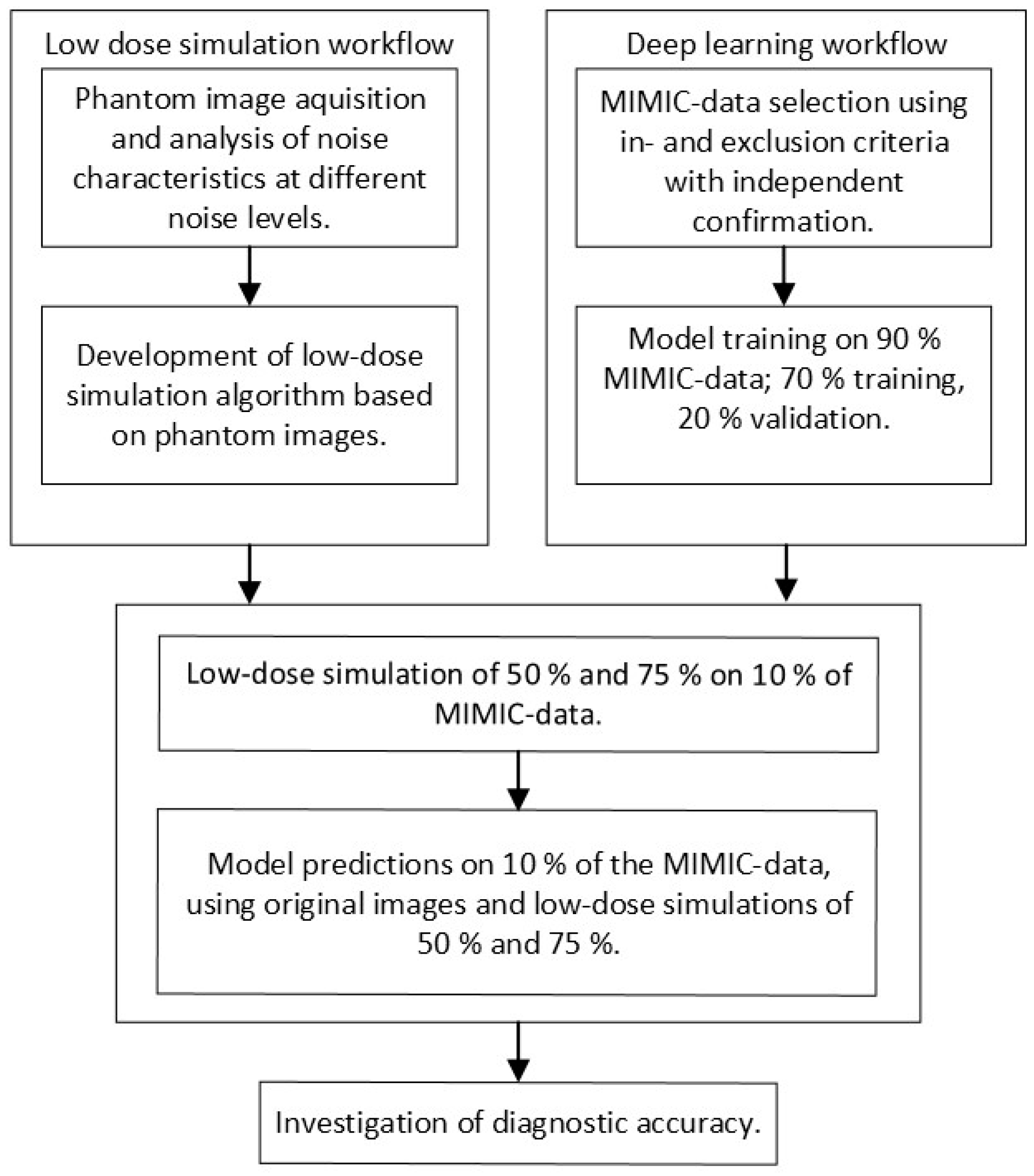
This study was performed in four steps, which are schematically represented in
Figure 1. First, a low-dose imaging simulation procedure was developed based on X-ray images obtained for this study using an anthropomorphic phantom. This simulation made it possible to process a single examination at different dose levels. Second, the MIMIC dataset, containing original chest radiographs, was used to train CNNs. Third, the developed low-dose simulation was applied to 10% of the MIMIC radiographs for independent testing. Fourth, the effect of simulated dose reduction on CNN performance was investigated. During the investigation, subpopulations were considered by stratifying for gender (male and female) and positioning (posterior–anterior (PA) and anterior–posterior (AP)).
2.1. Simulated Low-Dose Imaging
To analyze the relationship between noise and exposure parameters, a set of chest images was acquired using an anthropomorphic Alderson phantom containing tissue-equivalent materials representing different organs. A common range of clinically relevant exposure parameters for chest radiography was used with tube voltages (80, 100, and 120 kVp) and manual exposure time products (0.6, 0.8, 1.2, 1.6, and 2 mAs), resulting in 15 separate images. Note that the tube voltages within MIMIC have a mean (SD) of 101 (±12) kVp and fall within this range. All images were acquired at a source-to-image distance (SID) of 150 cm. This approximates the distances used in the MIMIC dataset, which are 183 (±0.6) cm and 165 (±3.2) cm for PA and AP images, respectively. The resulting phantom images were analyzed using 10 × 10-pixel sliding windows to measure the mean and standard deviation of the grey values, representing an approximation of noise. Linear regression was used to approximate the relationship between the mean grey values (horizontal axis) and standard deviation (vertical axis) for each tube voltage and exposure time product combination. To overcome systematic error in direct exposures, where grey values are 0 and the standard deviation is negligible, the x- and y-axis intercepts were set to 0. The resulting regression slope represents the variation in SNR per anatomical region caused by a variation in attenuation for each 10 × 10-pixel window. The slopes of lower-dose images were used as a ‘goal slope’ to create dose reductions from the original-dose images per tube voltage.
The ‘goal slope’ derived from the phantom images was used in a custom Python (version 3.7) script to introduce generated noise on images (hereafter referred to as InGen). InGen implements three steps to add noise to existing X-ray images, such as those available in MIMIC.
First, the original-dose full-resolution images were divided into twenty equal-sized grey value threshold windows (e.g., 0/20th–1/20th, 1/20th–2/20th, etc.). These twenty thresholds were determined during a preliminary phase and based on the visual inspection of simulations with various numbers of thresholds. For each window, the mean grey value was multiplied by the ‘goal slope’ related to the intended low dose. This outcome was multiplied by an array of randomly generated values between 0.0 and 1.0, taking the same size as the image. Combining these multiplications resulted in a noise mask.
Second, the resultant noise mask was further adjusted to increase visual agreement with real noise by using a multiplication factor of 6 or 9 to adjust the noise level to the ‘goal noise level’ of the phantom images. These multiplication factors were determined during the preliminary visual inspection while comparing the resultant slope to the ‘goal slope’, ensuring clinical representation of the generated low-dose simulations. Further optimization was performed by applying a zero-centered Gaussian filter with unit standard deviation to soften the noise.
In the last step, the processed noise mask was added to the original image, after which a correction was applied to restore the range of grey values present in the original image. This step, based on grey value thresholding followed by histogram correction, is crucial as it ensures that the grey values in the simulated low-dose image match those of a normal exposure, which were lost by subtracting the noise mask. The result is a simulated low-dose image that replicates what was initially an image with normal exposure.
The above steps were performed using Python 3.7 in combination with Scipy (version 1.4.1) and Skimage (version 0.16.2).
2.2. AI Model Training
The datasets MIMIC-CXR v2.0.0, -JPG 2.0.0, and -IV v0.4 were used for training [
28,
29,
37]. These consist of anonymized patient information (e.g., date of birth and gender), full-resolution and full bit-depth DICOM-format chest radiographs, and their fourteen corresponding diagnoses. Each of the fourteen diagnoses is expressed as a binary label, each indicating the presence or absence of the related pathology. All MIMIC data were used in accordance with the PhysioNet Credentialed Health Data Use Agreement 1.5.0.
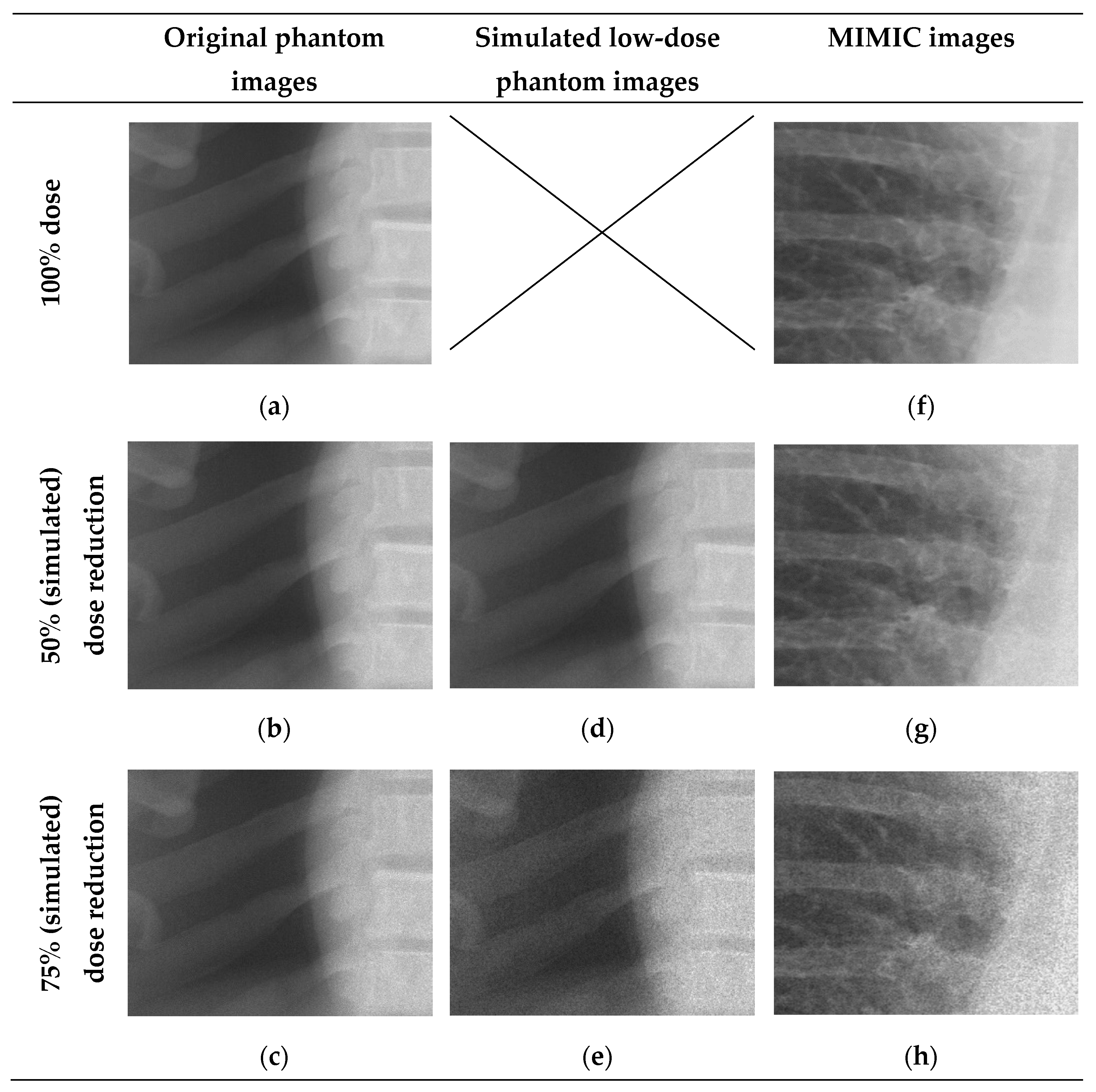
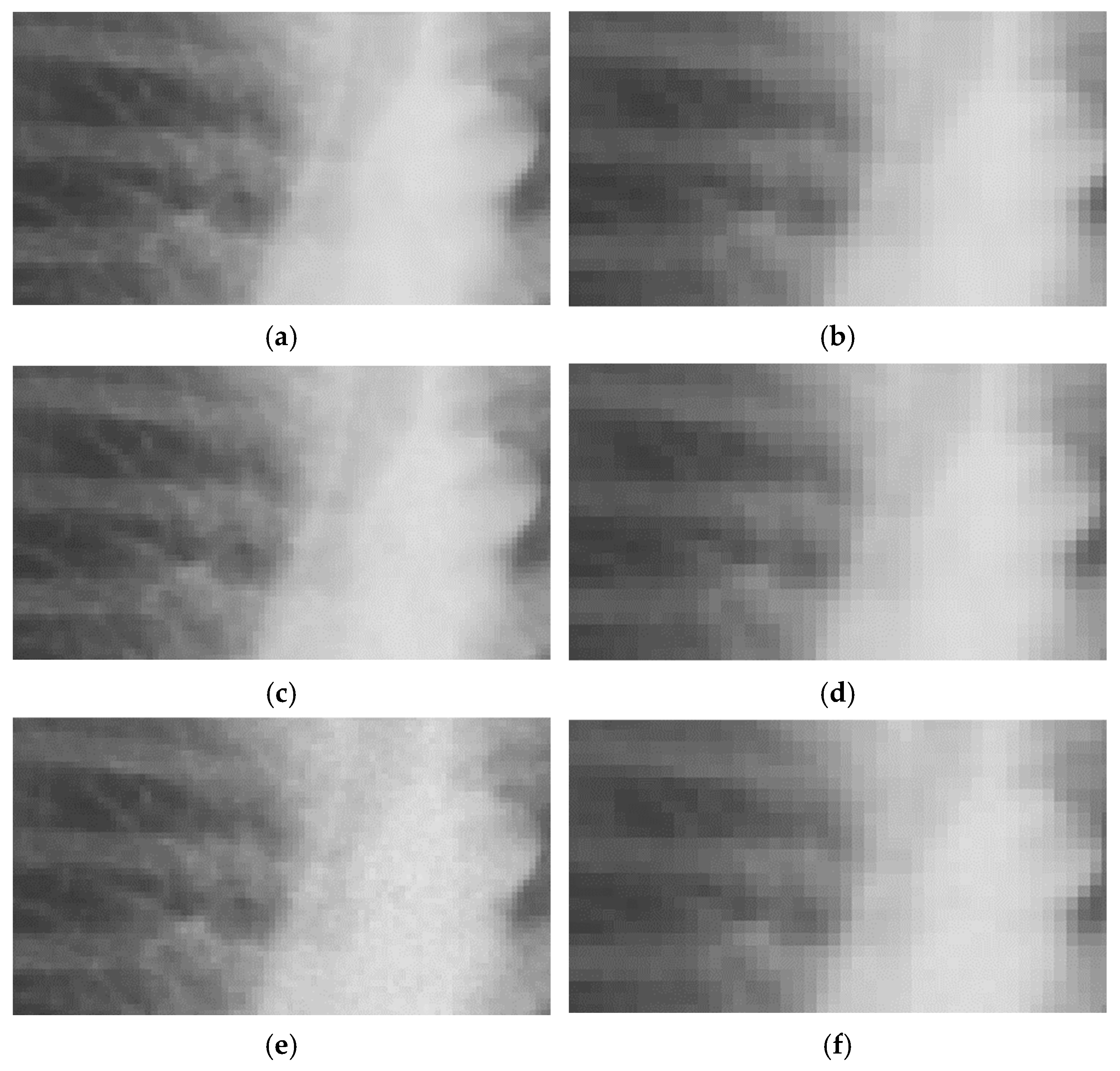
The primary data source of this study is the MIMIC-CXR containing 227,835 chest radiographs. Examples of these images are shown in the Results section (see
Figure 2 and
Figure 3 for close-ups and
Figure 4 for images of varying quality). The corresponding pathology labels for the images in MIMIC-CXR were taken from MIMIC-CXR-JPG [
29,
37]. Metadata from the MIMIC-CXR DICOM images were extracted using Pydicom (version 1.4.2). The relevant variables derived were tube voltage (kVp), exposure time product (mAs), dose area product (DAP, unit unknown), exposure index (EI), relative exposure index (REX) (collectively referred to as exposure parameters), and ‘acquisition date’. Both ‘anchor age’ and ‘anchor year’ from MIMIC-IV were used in combination with the ‘acquisition date’ from the DICOM metadata to derive the patient age at the time of exposure [
36].
The inclusion and exclusion of pathologies and related images were performed by the first author, a radiographer with over ten years of experience, and validated using the literature [
21,
38,
39,
40,
41]. Of the fourteen available pathologies, eight were included based on clinical relevance: No Finding, Fracture, Enlarged Cardiomediastinum, Cardiomegaly, Atelectasis, Edema, Pneumonia, Lung Lesion (see
Table 1). Pneumothorax was excluded because of the presence of drains on 30% of 100 random pneumothorax images. Previous studies have shown that drains cause an overfit in CNN development related to pneumothorax [
33,
38]. Secondly, ambiguous language or limited difference in image characteristics lead to the exclusion of Lung opacity, Consolidation, Pleural other and Pleural effusion [
29,
33]. Lastly, images positively labelled under Support Devices were excluded from classification due to limited clinical relevancy. A radiologist with over twenty years of experience independently confirmed the choices made.
Only pathology labels with clear certainty were included (1 and 0). The uncertain label (−1), occurring in 2% of the cases was excluded, limiting the inclusion of false positives or false negatives [
24,
29]. The presence/absence labels were taken as true positives (1) and true negatives (0) during the training and validation of the CNNs. Additional exclusion based on image quality was not performed to circumvent an overfit on clinically unrealistic image quality.
For each of the seven pathologies, image sets were created, with 50% of the images showing the presence of the specific pathology and 50% showing its absence. Each image set was limited to one pathology label, resulting in seven separate pathology-based image sets. The maximum size per image set was 10,000 images, and each set was saved separately. The final number of images used for training, validation, and testing per pathology ranged from 4670 to 10,000, depending on the number of images available for each pathology (see
Table 2). These image sets were randomly divided into training, validation, or test sets with a split ratio of 0.7, 0.2, and 0.1, ensuring independence among samples.
The training was performed on an EfficientNetB4 model pretrained with ImageNet using Keras (version 2.4.3) with a TensorFlow (version 2.4.1) backend [
42]. This model was customized with a top layer (Dropout (0.2), Flatten, and Dense (1) with sigmoid activation) to facilitate binary classification per pathology.
The resolutions used were based on the approach by Sabottke et al. and available hardware resources, in which a batch of four could be used at 254 px × 305 px and a batch of eight could be used for 127 px × 152 px (respectively referred to as low resolution (‘LR’) and ultra-low resolution (‘ULR’)) [
33]. A custom image data loader was used to allow for the use of 16-bit images and augmentations to simulate a broad range of geometric image acquisition variations. The implementation of image augmentation was based on the literature and was applied by Keras in its built-in augmentation during the training phase, which included a rotation ± 10 degrees, vertical flip, and fractional changes to the zoom range ± 0.01, height shift ± 0.05, width shift ± 0.1, and shear range ± 0.1 with a ‘constant’ fill mode [
39,
40,
41,
43]. Note that no augmentations were applied during testing to ensure independence of the impact of the simulated low dose on CNN performance during testing.
The values of the hyperparameters for model training were based on the literature and tuned through preliminary testing [
33,
39,
40]. The implementation of an Adam optimizer with an initial learning rate of 1 × 10
−3 and binary cross entropy loss function led to the optimal reduction in validation loss during these preliminary tests. Additionally, preliminary testing led to the implementation of a learning rate scheduler and an adjustment in the number of steps per epoch. The learning rate scheduler reduced the learning rate by a factor of 0.5 after each epoch, while the number of steps was reduced by a factor of 4 to increase the effect of backpropagation (therefore, each epoch was a ‘semi-epoch’). Preliminary experiments pointed towards stabilization in the training process after six epochs.
The resulting fourteen separate models, created by crossing seven pathologies with two resolutions, were trained end-to-end. Each model predicted the presence of a pathology using a range between 0 and 1. Predictions close to 0 indicated that the pathology was absent with a high certainty, while those close to 1 indicated that the pathology was present with a high certainty.
An overall investigation of the impact of simulated low-dose imaging on CNN performance was achieved by applying InGen to all images within the test image sets. Simulations were based on the ‘goal-coefficients’ and correction factors from the phantom images. Both types of parameters were based on a tube voltage of 100 kVp, taken from the MIMIC-CXR meta-data. Three separate dose levels were simulated for both LR and ULR resolutions: one for the original image dose and two for the simulated dose reductions of 50% and 75% using InGen. Please note that these simulated reductions represent images with 50% and 25% of the original dose.
2.3. Data Analysis
A visual face validity check was performed to investigate the clinical representation of simulated doses by using 15 randomly selected images. The corresponding author and an experienced radiologist independently performed this check. Additional image quality investigation was performed using the structural similarity index (SSIM) and peak signal to noise (PSNR). Both SSIM and PSNR were determined for the original resolution, LR and ULR [
44].
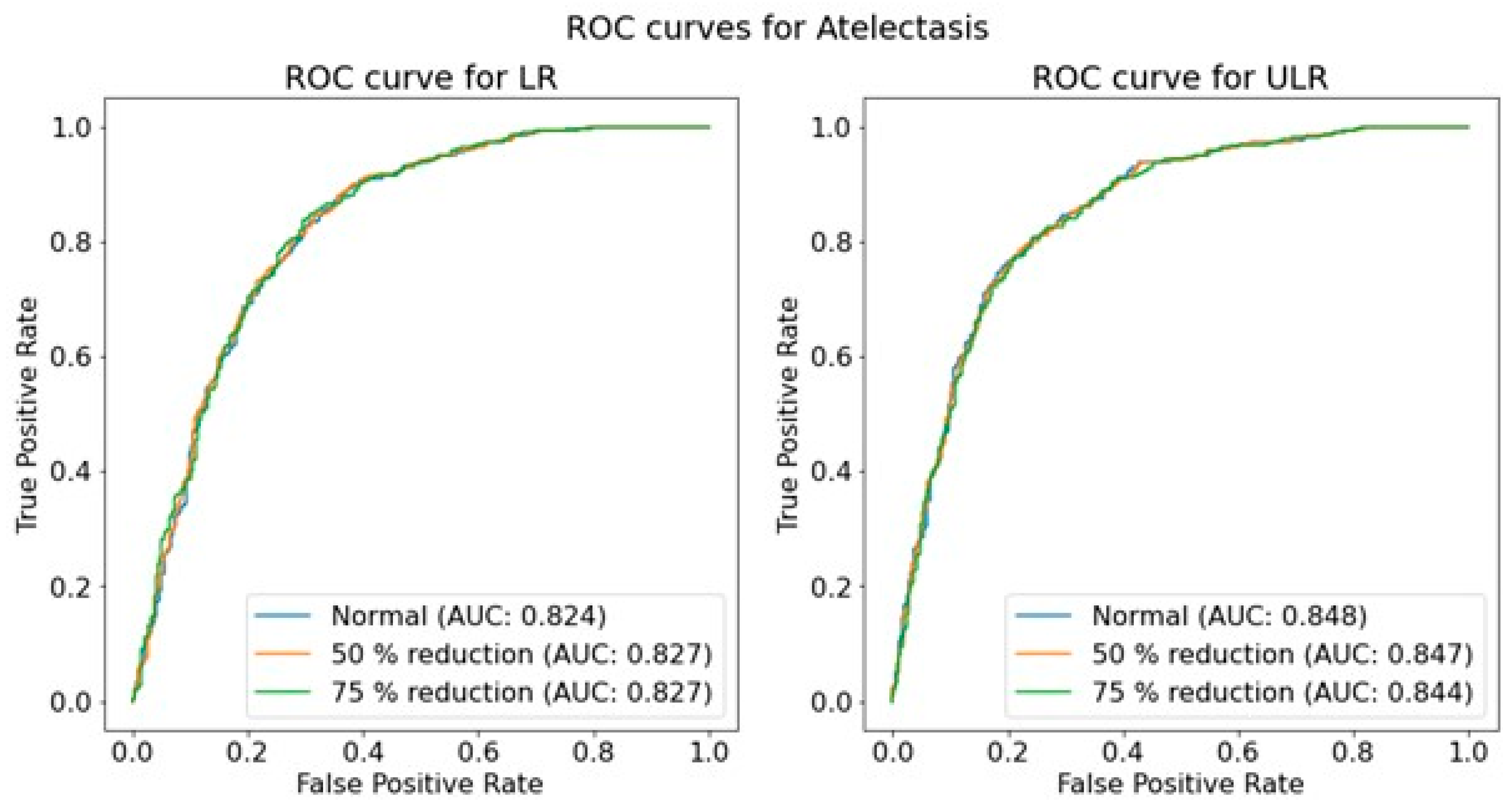
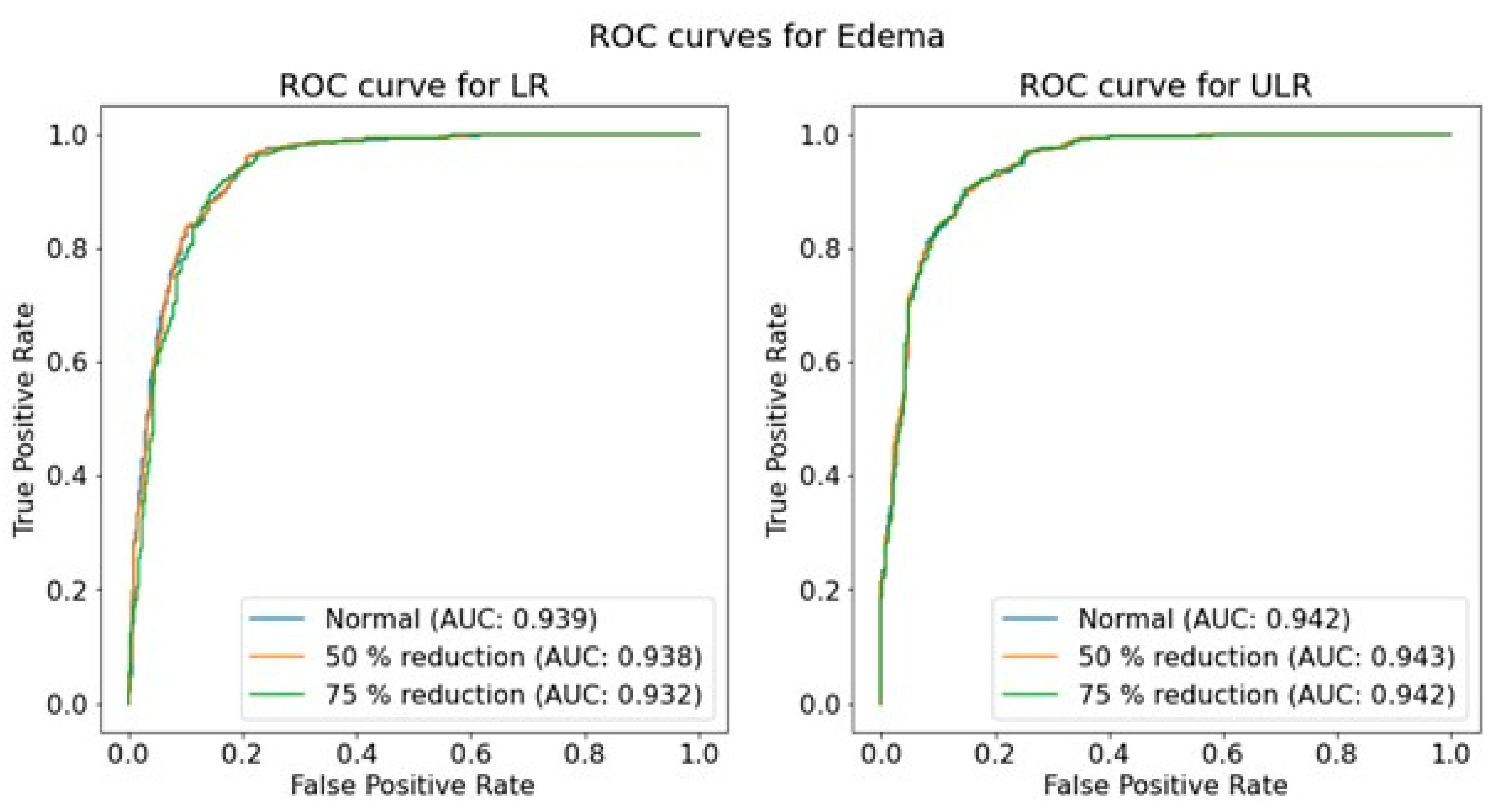
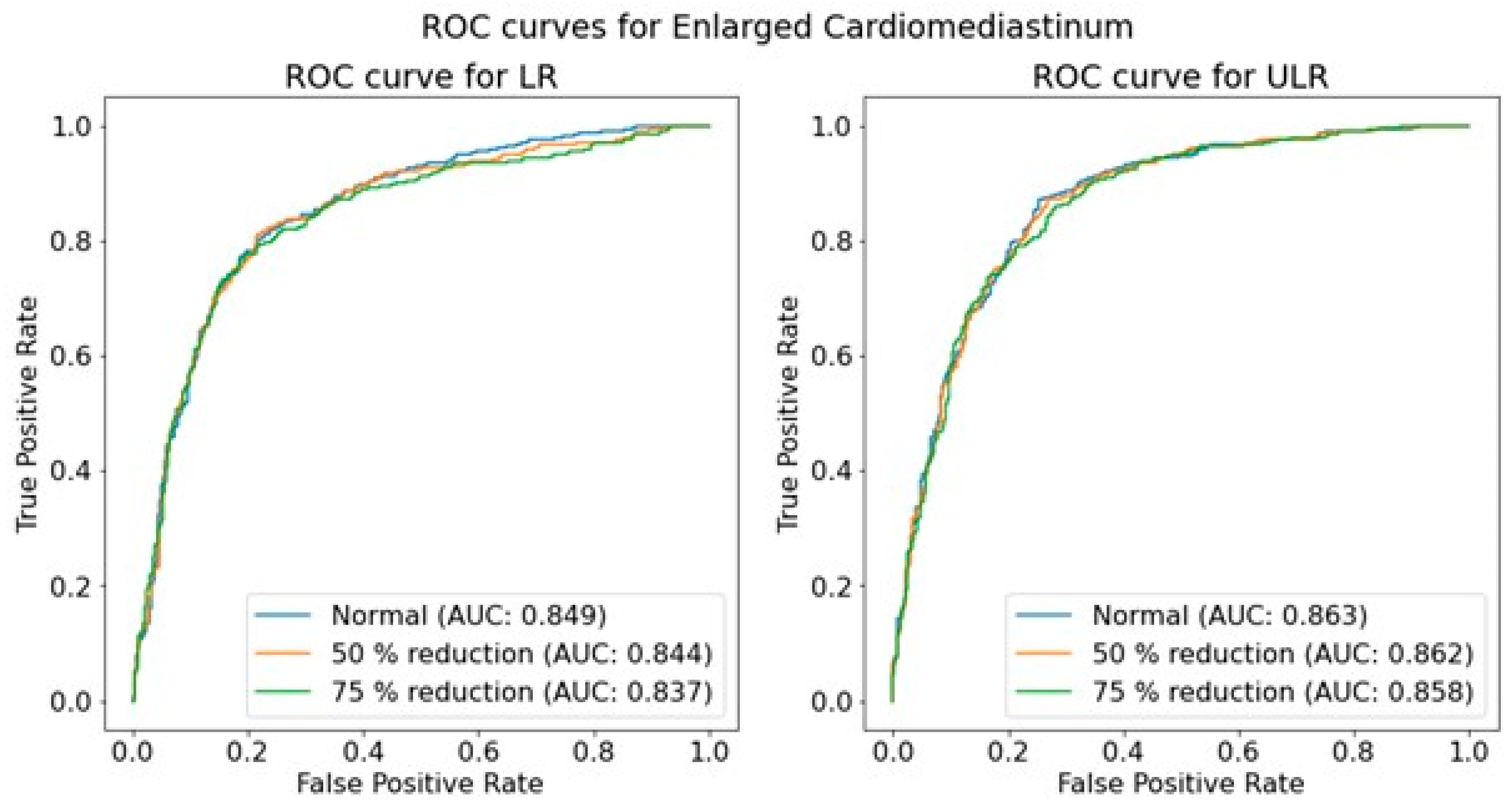
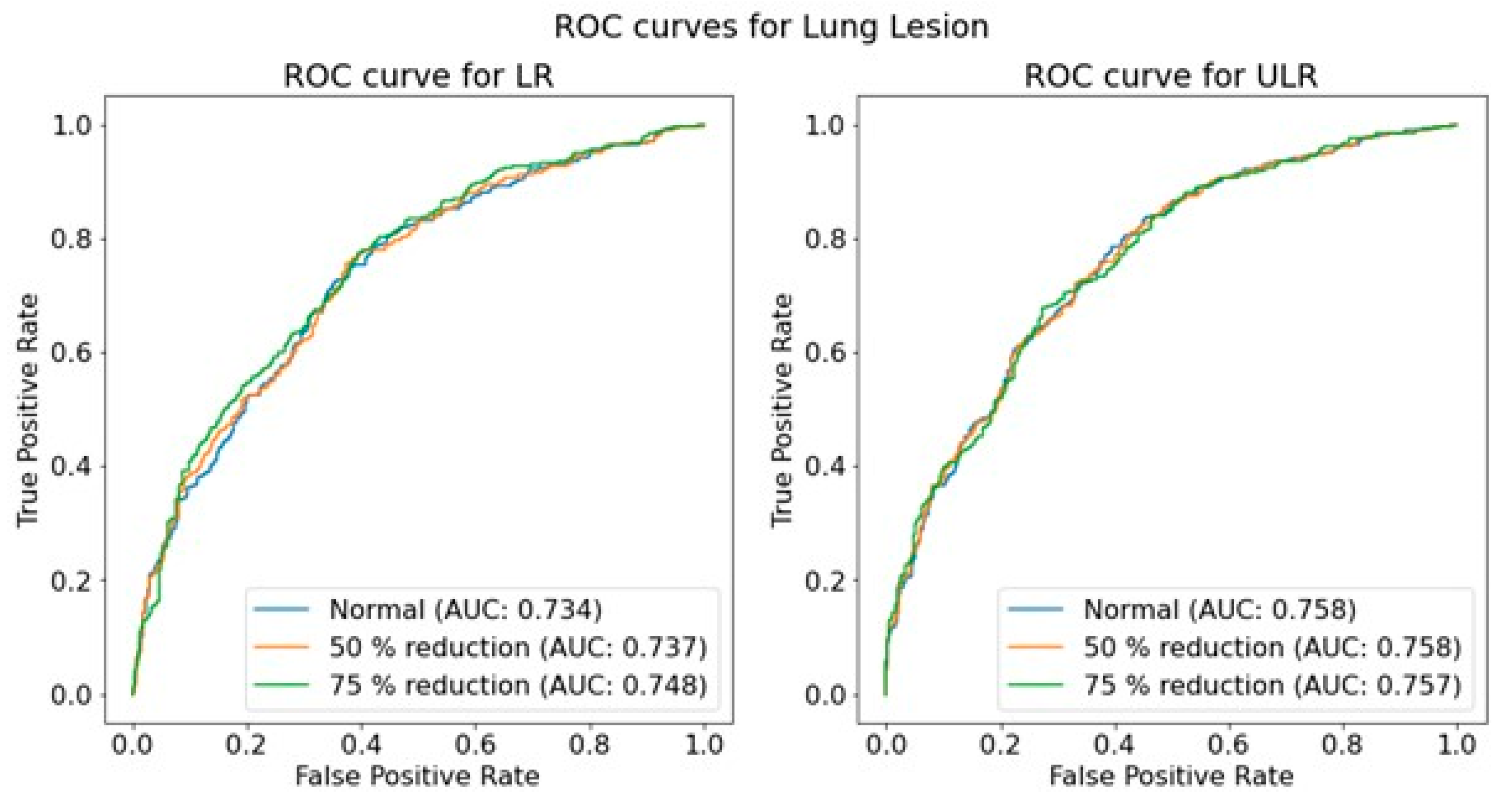
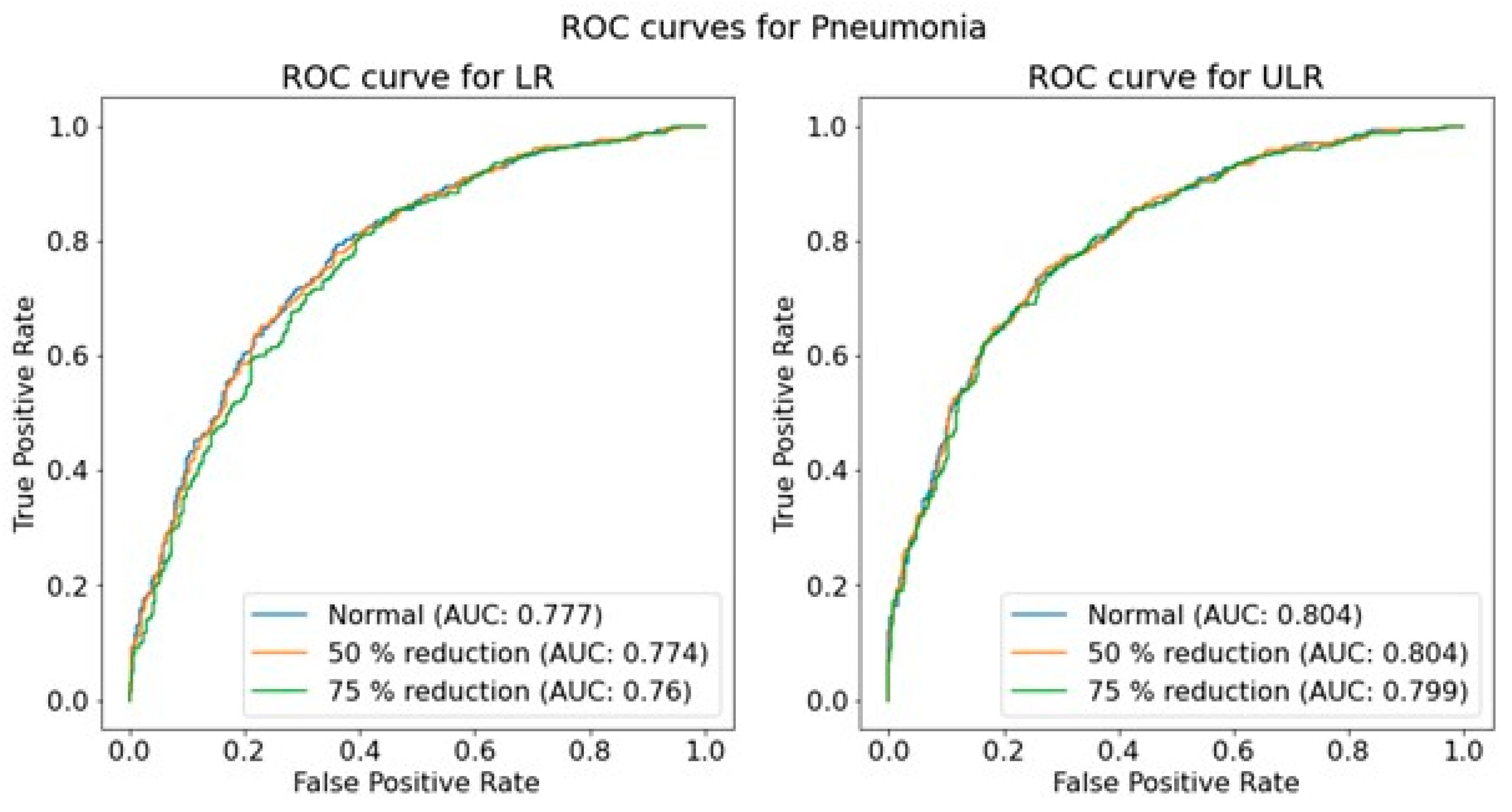
The performance of the trained CNNs was operationalized using the AUROC obtained from predictions on independent test sets for each pathology, resolution, and dose level. The use of AUROC facilitates comparison with relevant literature and, due to its monotonic relationship with sensitivity and specificity, a higher AUROC indicates better clinical performance. To assess the significance of the effect of simulated dose reductions on CNN performance, the ROC curves of the original image predictions were compared to those of the simulated dose reductions using a DeLong test [
45,
46]. This comparison was performed for both resolutions independently, and for each of the seven pathologies.
To provide insights into potential clinically relevant outcomes, additional preliminary investigations were carried out. The differences in exposure parameters and age for PA and AP positioning were tested using a Mann-Whitney U test for continuous non-normally distributed data. Analyses were performed using Scikit-learn (version 0.22.1) to determine the AUROC and SciPy (version 1.4.1) for all other statistical analysis with a significance level of p < 0.05.
Finally, a cursory estimation on overall image quality related to image acquisition was performed on 100 random images for both AP and PA positioning.


 ,
, 


