Abstract
This paper proposes the transformation , where S is a digital gray-level image and is a vector expressed through the textural space. The proposed transformation is denominated Vectorial Image Representation on the Texture Space (VIR-TS), given that the digital image S is represented by the textural vector . This vector contains all of the local texture characteristics in the image of interest, and the texture unit entertains a vectorial character, since it is defined through the resolution of a homogeneous equation system. For the application of this transformation, a new classifier for multiple classes is proposed in the texture space, where the vector is employed as a characteristics vector. To verify its efficiency, it was experimentally deployed for the recognition of digital images of tree barks, obtaining an effective performance. In these experiments, the parametric value λ employed to solve the homogeneous equation system does not affect the results of the image classification. The VIR-TS transform possesses potential applications in specific tasks, such as locating missing persons, and the analysis and classification of diagnostic and medical images.
1. Introduction
Visual texture is an important element for component classification in scenes and is commonly used for the processing of visual information. The surfaces of all materials are characterized through their texture properties, which can be described as follows: (a) the visual texture is a spatial distribution of gray levels; (b) the visual texture can be perceived through different scales or resolutions; (c) the texture is an area property and not a point property; (d) a region is perceived as texture when the number of primitive objects within it is large. On the other hand, according to reference [1], some important perceptions in the quality of a texture are uniformity, density, rugosity, linearity, direction, frequency, and phase. Henceforth, a texture can be considered as fine, rough, soft, regular, irregular, or linear. The grade of irregularity or the properties of a texture can be found scattered throughout the entire image. In the field of texture analysis, there exist three major problems: (a) texture classification, focused on determining to which class the sampled texture belongs [2,3,4]; (b) texture segmentation, where an image is sectioned into multiple regions and each region has a specific type of texture [5,6]; and (c) texture synthesis, which focuses on constructing a model that can be employed to produce artificial textures for specific applications such as computer graphics [7,8]. Furthermore, according to reference [9], the characteristics extraction techniques can be classified into three categories: geometrical methods, signal processing, and statistical models. Geometrical methods are based on the analysis of primitive textures. Some geometrical methods for primitive extractions include adaptative region extractions, mathematical morphology, structural methods, and border detection [10,11]. The model-based methods hypothesize the subjacent texture, constructing a parametric model that can generate the intensity’s distribution of interest. Ergo, these models can also be employed for texture synthesis. Some of these models that are applied for texture synthesis are called stochastic spatial interaction models, random field models, and fractals [12,13]. The signal processing methods perform an analysis of the frequency components of the images; the latter are also known as filtering methods, and to mention only some of these, we submit spatial domain filter, frequency analysis, and spatial/spatial–frequency methods [14,15]. Last but not least, the statistical methods offer an analysis of the spatial distribution of the local texture characteristics. Such characteristics are represented through a histogram of a variable dimension depending on the procedure employed to calculate the texture unit [16,17,18]. This histogram presents the occurrence frequency of the estimated texture units within the digital image, and its dimension is dependent on the unit texture definition. Selection of the texture extraction method is conducted in agreement with the problem under consideration. There are two types of classifiers for image classification in an a priori knowledge scheme: one-class and multiclass. For one-class classifiers [19,20], an unequivocal class is clearly defined, while the remaining classes are of no interest. In this situation, a region is defined within the characteristics space; this region represents the textural characteristics of the known class. This region is the acceptance zone for the class of interest or is employed as a prototype. On the other hand, in the multiclass classifiers [21,22,23], the characteristics space is divided into multiple regions, each region corresponding to the characteristics of a class and, frequently, the class (image) is represented by a characteristics vector known as a prototype vector. The classification of multiclass images consists of comparing the characteristics vector of a test image with the characteristics vectors of the known classes. Henceforth, the test image is assigned to the class with the most similar characters. This discrimination is performed by means of finding the distance between the vectors within the characteristics space.
To our knowledge, the texture unit has not been defined through a homogeneous equation system, which is defined through an observation window. In this paper, the local texture characteristics are extracted from grayscale images . To extract the texture characteristics, a mobile observation window of in size is employed to detect local random patterns of pixels across the image. In each detected position, the pixel values are considered constants within a homogeneous equation system whose solution is the vectorial unit texture . This unit is represented in a new texture space as a vector radius that extends from the origin to the vector position , such that each random pattern of pixels has a corresponding texture unit vector (vector radius). By adding together all of the components of the vector radius, is calculated; this latter vector contains all of the local texture characteristics of the image under study, S. Ergo, the transformation represents a gray-level image S through a vector , whose direction and magnitude depend entirely on the textures of the image. This transformation has been denominated Vectorial Image Representation on the Texture Space (VIR-TS), due to the representation of a digital image S through the vector . The efficiency of the VIR-TS transform was experimentally corroborated through the classification of tree stem images with a multiclass classifier, where the vector is employed as a characteristics vector.
The report has the following structure. Materials and methods are presented in Section 2. In Section 2.1, the texture space is described based on three subsections: Section 2.1.1, the definition of the texture unit is shown; Section 2.1.2, the definition of the texture unit is represented graphically; and Section 2.1.3, the representation of a digital image in texture space is described. In Section 2.2, the procedure to measure the similarity in texture space between a prototype vector and a test vector is explained. Section 2.3 describes a classifier for multiple classes in texture space and where the VIR-TS vector is used as a feature vector. In Section 3, the experimental work is developed. In Section 3.1, a digital image database is vector-represented in texture space where each vector has its own direction and magnitude. Furthermore, using the vectors obtained in the transformation, the similarity between images is measured. In Section 3.2, experimental results of image classification are reported, which demonstrate the high efficiency of the VIR-TS technique. A discussion of our work is provided in Section 4. Finally, in Section 5 the most relevant conclusions are presented.
2. Materials and Methods
2.1. Texture Space
2.1.1. Texture Unit Definition
In the texture analysis, a mobile observation window W frequently bears a size [21,24,25]; it is deployed to extract the local texture characteristics of an image under study. This window is shifted pixel-by-pixel across the whole image and, for each position, the window detects a discrete pattern, which is employed to generate a decimal code called a texture unit. Afterward, the texture unit is interpreted as a discrete variable and is then taken as an index to generate a discrete histogram . Such a histogram is interpreted as a texture spectrum and is then deployed as a characteristics vector in image classifiers [21].
Now, bearing in mind the structure of the mobile observation window, and considering the gray-level image such as a random matrix , with size , and for each position, a discrete pattern is detected through the window, as shown in Figure 1. If the pattern elements are considered the coefficient of a homogeneous equation system, the system will be:
where is termed the coefficient matrix of the homogeneous linear system, represented as a matrix of real elements, and is called the unit texture vector. The trivial solution of the homogeneous equation system occurs when all of the elements of vector have a value of zero: , , . Nonetheless, this solution is not functional for our interests; thus, a nontrivial solution must be found. Therefore, based on a linear algebra concept, the nontrivial solution is possible when its determinant is equal to zero; as a consequence, there will be infinite solutions. To achieve this, the term is introduced within the equations and their determinant is equal to zero, as shown in Equation (2):
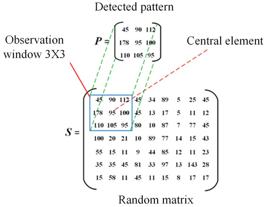
Figure 1.
A pattern P detected in the grayscale image S through an observation window of 3 × 3 elements.
Hence, the problem becomes that in finding a K value, so that the condition is satisfied. From Equation (2), in terms of the matrix elements , K has a value of
Once the value K is determined, it is introduced into the equation system; Equation (1) then takes the following form:
where the value is determined by Equation (3).
Afterward, to determine the texture unit , the nontrivial solution of Equation (4) must be found. As a first step, the first two linear equations are left depending on :
employing the Cramer Rule method, the solution for is obtained through:
while the solution for is:
where D is the determinant of the 2 × 2 equation system, is the determinant for , and is the determinant for . It is noteworthy that and function on the basis of ; accordingly, the infinite solution in parametric form is:
Observing Expression (8), for each real value of lambda , a unique resolution of the infinite solution is found. For example, when , the trivial solution of the equation system is obtained (, , and ); henceforth, the nontrivial solution is obtained when .
2.1.2. Graphical Representation
Based on Equation (1) and Expression (8), the unit texture vector is defined by: It can be represented through the Cartesian coordinate system form:
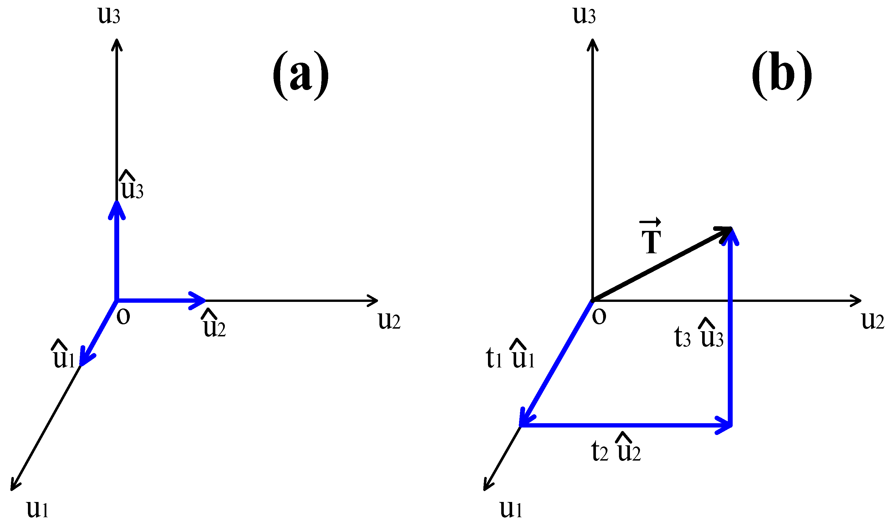
where , , are the unit vectors that indicate the axis direction in a rectangular coordinate system of three dimensions (Figure 2a). Hereafter (9), the scalars are the components of vector in the directions . Finally, from Equation (8), the magnitude of vector is:
and its directing cosines are:
where
with being the magnitude of vector ; its graphic presentation is displayed in Figure 2b. Based on Figure 2b, the texture unit is a radius vector that extends from the origin to the coordinates .
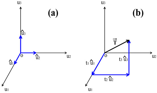
Figure 2.
Representation of unit in the texture space: (a) graphic representation of unit vectors , , ; (b) graphic representation of texture unit and its components .
It is clear that the direction and magnitude depend on the λ value and the elements in the pattern.
2.1.3. Image Representation on the Texture Space
Given that, if a grayscale image S has an size and if this image is analyzed through an window, then there are patterns . Furthermore, given that each pattern (in the image domain) generates a texture unit (in texture space), then when the image is analyzed locally through the observation window for the pattern , the texture unit is calculated (radius vector in texture space); as a consequence, the image can be represented through a series of radius vectors. Thus, adding together all of the components of all of these radius vectors in the texture space, the image is represented by vector , defined as:
The directions are given by and the components are calculated with:
where is the component of the elements for , is the component of the elements for , and is the component of the elements for . Equation (9) was considered, and is the total of the patterns found in the digital image under study. Figure 3 depicts vector , which is in texture space.
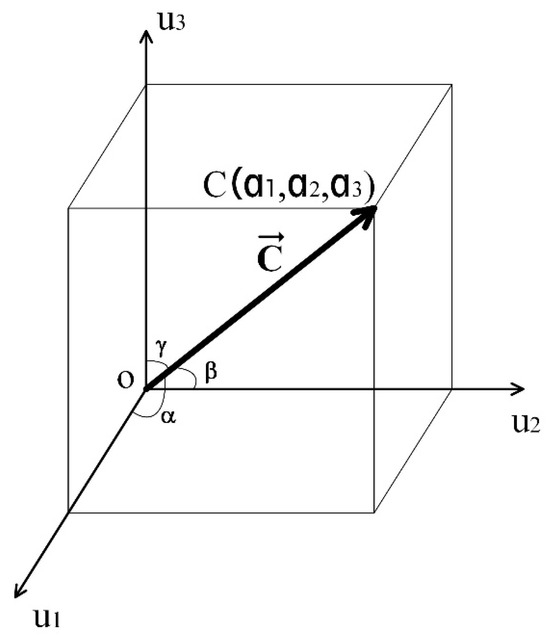
Figure 3.
Graphic representation of the texture vector with its directing cosines.
Considering Figure 3 and Equation (13), the magnitude of vector is:
where its directing cosines are given with:
and holding the equivalence:
Based on the performed analysis, image can be represented as a radius vector in the texture space whose magnitude and direction depend on the randomness in the image under study.
2.2. Similarity Measurement between a Prototype Image and Test Image
With the knowledge that the transformation is possible, then the measurement of similarity between a prototype image and an unknown test image can be performed in the texture space.
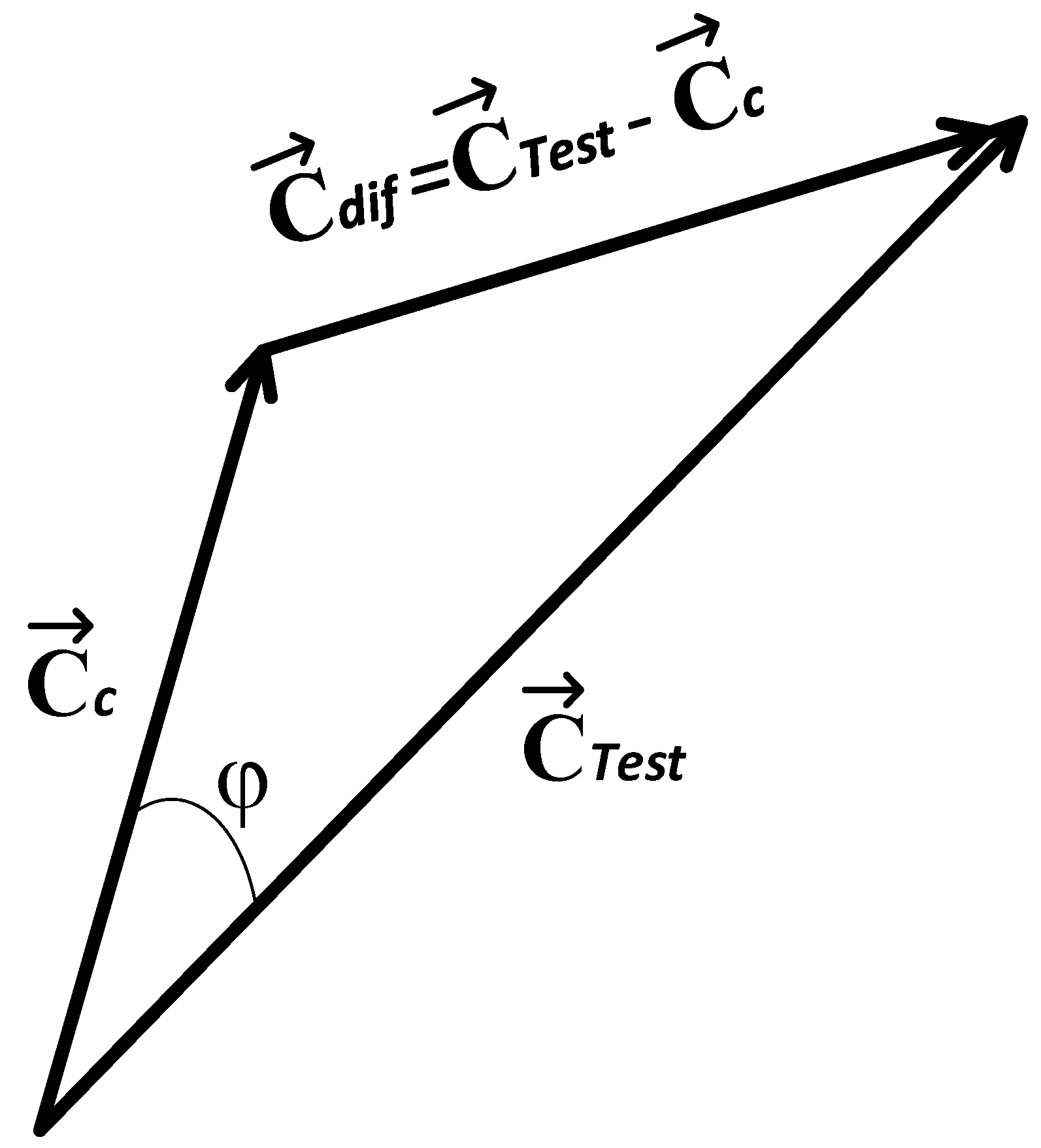
Given a digital image of a c class whose texture vector is , and given an unknown test image whose vector is , the difference between the and images in the texture space can be calculated through subtraction of the unknown image minus the vector of the prototype image :
where is the difference vector between the texture images.
Images deploy the and vectors. Considering the cosines law and the geometry present in Figure 4, we obtain:
and from (19), we obtain:

Figure 4.
Geometry employed for the similarity measurement between and .
Due to the geometry of the problem, if (18) is substituted in (20), we obtain:
On applying the distributive law:
On reducing, we reach
From (23), the following relationship can be achieved:
where the symbol indicates a scalar product, is the magnitude of vector , is the magnitude of vector , and is the cosine of the angle formed between the and vectors. With the knowledge that Expression (24) is employed to measure the similarity between vectors, this equivalence is achieved:
where sim(S_Test, S_c) is the similarity measurement between the and images. Thus, based on Figure 4 and Equation (25), the following conditions (as points) can be indicated:
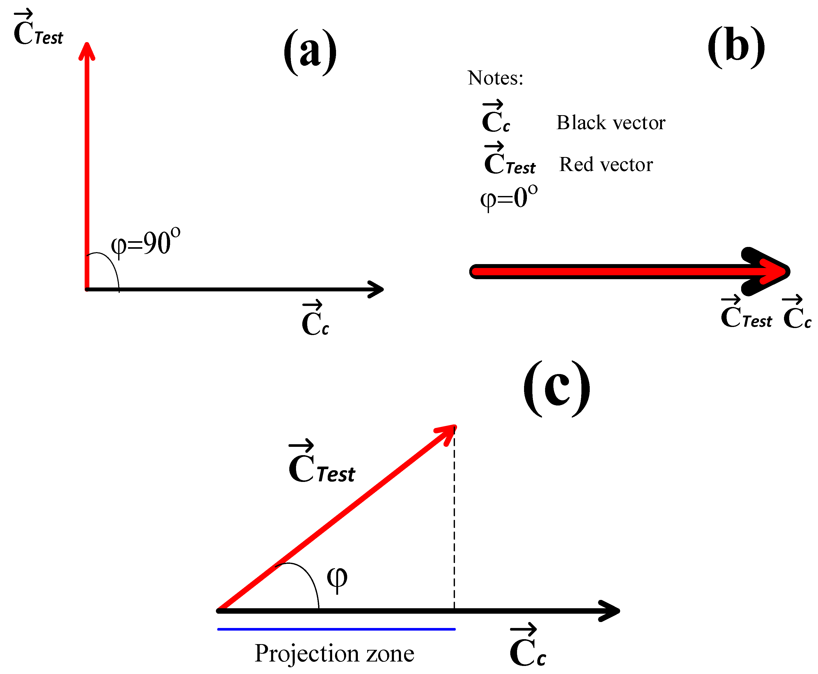
- If , then , because and are orthogonal, . Ergo, the and images are completely different (see Figure 5a).
 Figure 5. (a) The and the vectors are orthogonal, and the similarity of and equals 0. (b) The and vectors are parallel; hence, the and images are identical, and (c) there is a certain angle between the and the vectors; thus, the and images possess a certain degree of similarity.
 - If , then , because and have the same direction and magnitude, . For this case, the and images are identical (see Figure 5b).
- If then ; consequently, the and images have a certain degree of similarity between them, given that the and vectors are not parallel within the texture space. Therefore, the condition is satisfied (see Figure 5c).
Based on conditions 1–3 and on Figure 5, it is possible to measure the similarity between images within the texture space; therefore, texture image classification is also a possibility.
2.3. Image Classification in the Texture Space
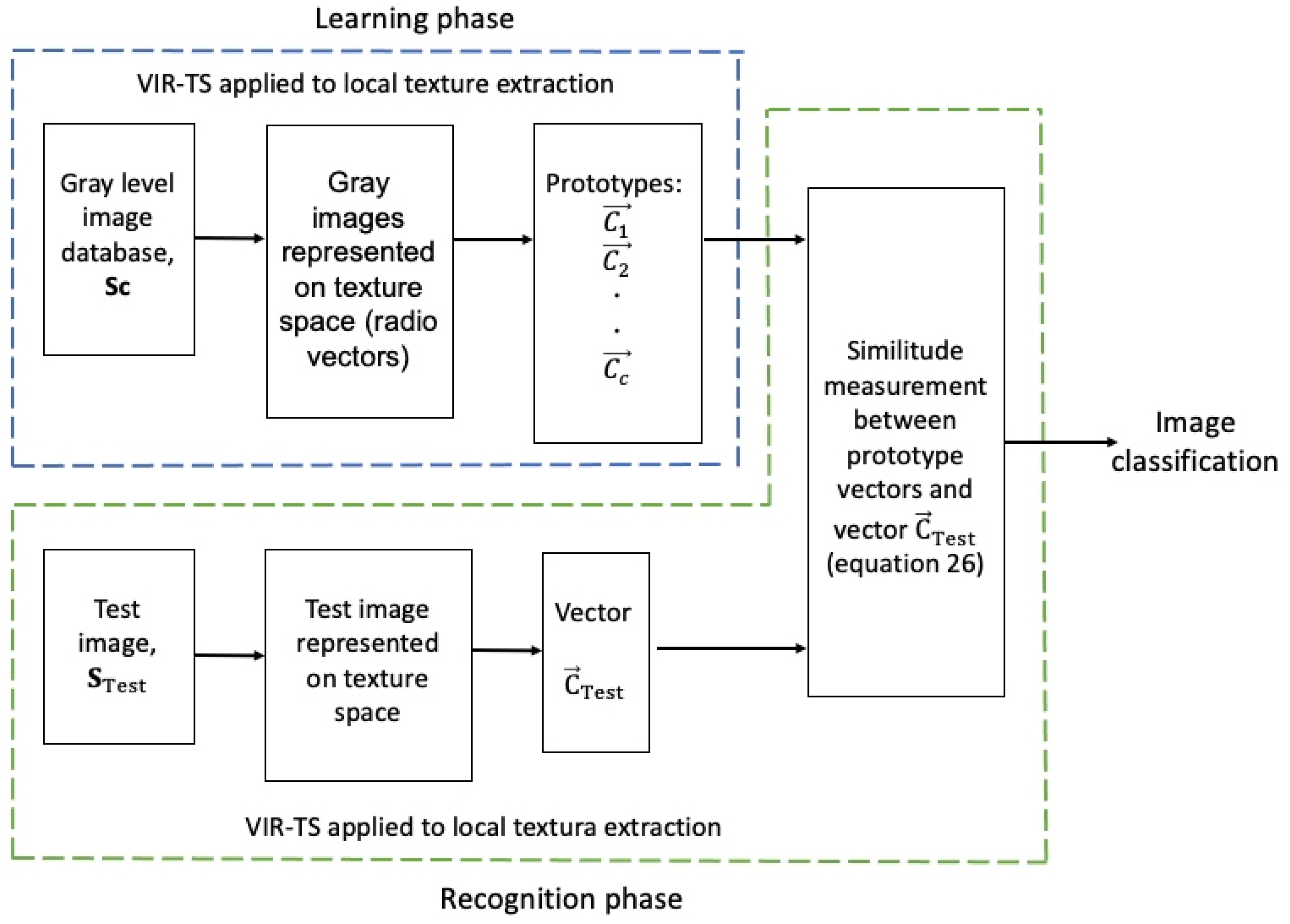
Figure 6 schematically displays the proposed multiclass classifier for image recognition within the texture space. The classifier consists of two phases: learning and recognition. During the learning phase, a human expert identifies and names a known image database , where each image is considered as an independent class; each class has a series of radius vectors that are calculated, and with these radius vectors, the prototype vector is obtained. This vector represents all of the local texture characteristics of the image within the class. In the recognition phase, an unknown test image is represented through a series of radius vectors and the vector is calculated with these. Afterward, the similarity between the test image and the prototype images is measured in the texture space employing Expression (25). The test image is then assigned to the most similar class; such a condition is achieved when the angle y is the smallest of these during the comparison between the and vectors (see Figure 5) and when the following condition is satisfied:
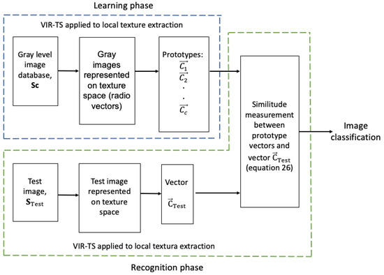
Figure 6.
A schematic representation of the multiclass classifier.
Ergo, the image is assigned to the class when the projection of the vector above the vector is the unit or that closest to the unit.
The classifier results are displayed in a confusion matrix ; the rows show the prototype images, the columns show the test images, the elements of the main diagonal correspond to the correct classification hits, and the elements outside of the diagonal represent the classification errors. The classification efficiency in terms of percentage is calculated with:
where is the efficiency in terms of percentage, is the sum of all of the elements of the main diagonal in the confusion matrix, and is the sum of all of the elements within the confusion matrix.
3. Experimental Work and Results
3.1. Transformation of an Image Onto a Texture Vector
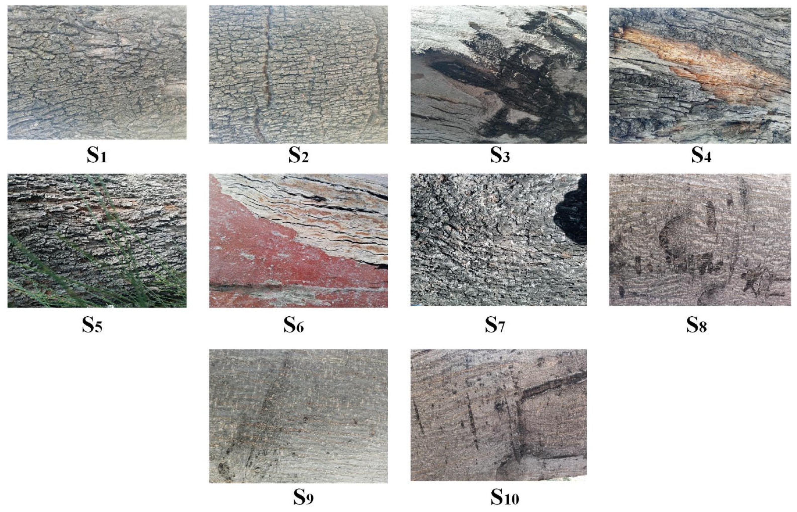
In this section, a database comprising 10 digital images of tree stems is represented through texture vectors , employing and values and an observation window of size. The database is presented in Figure 7. Each image was acquired with a Smartphone LG 50, and rotation and scale are controlled under natural illumination and with a fixed resolution of pixels.
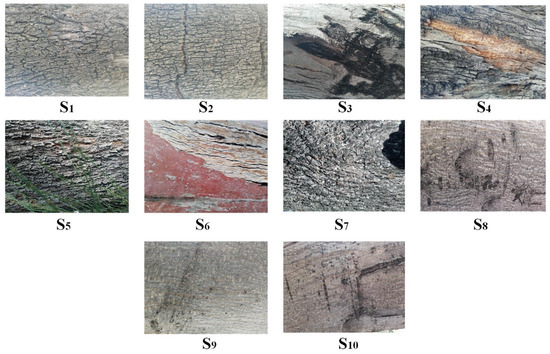
Figure 7.
Digital images of the tree stems employed in the experiments.
Additionally, the transformation was performed applying the following steps: (a) the RGB image acquired with the Smartphone LG 50 was transformed into a grayscale level deploying MatLab 2016b® scientific software; (b) an observation window with a size is selected; (c) the window is displaced element-by- element across the entire gray-level image with a size; (d) for each pattern , a homogeneous equation system is proposed, then its unit is calculated; (e) all units are represented in the texture space as a radius vector, and (f) by adding together all of the radius vectors, the vector is estimated. Exercising steps a–f, the images in Figure 7 were represented through a texture vector . The results are presented in Table 1.

Table 1.
Texture vectors obtained from the digital images shown in Figure 6.
Considering Figure 7 and Table 1, the digital image is represented in the texture space through a radius vector , whose components are dependent on the texture characteristics of the image and on the parametrization value . During the transformation, the texture characteristics of the image render the vector unique in the texture space, while the parameter operates as a scale factor.
To verify the uniqueness of each vector in Table 1, the similarity between these is measured employing the scalar product in Equation (25). The results are displayed in a confusion matrix, where the elements of the main diagonal correspond to the similarity measurements of the same vector hence, its value is the unit (marked in blue). Otherwise, the elements outside of the main diagonal correspond to the similarity measurement between two different vectors ; consequently, such elements have a value lower than the unit. Table 2 and Table 3 present these results:

Table 2.
Similarity measurement between vectors in the texture space, when λ = 2.

Table 3.
Similarity measurement between vectors in the texture space, when λ = 25.
Based on the results of Table 2 and Table 3, both confusion matrixes are identical, given that the elements in their respective diagonals are the unit, and the elements outside of their diagonals are fewer than the unit. This corroborates that a digital image is represented in the texture space through a unique vector , and that the parameter , operated as a scale factor and its value, does not affect the results. Furthermore, the similarity measurements between images above 0.94 are attributed to the parametrization of the homogeneous equation system due to its resolution. This causes the third component of all of the vectors to bear the same value , and the remaining two components (first and second) are the only components scaled by the value of (see Equation (8)).
3.2. Image Recognition in the Texture Space
Knowing that each digital image can be represented in the texture space through a vector, the goal of this section is to prove that the digital images can be classified in the texture space. As previously presented in Figure 7, the database consists of 10 digital images with a size of pixels; these images show the bark of tree stems and were acquired under natural lighting and controlled scale and rotation. The classifier employed for image recognition was described in Section 4. In both phases, the same images are employed for both learning and recognition, along with the same observation window size of pixels. The similarity measurement in the texture space is performed considering the maximal likeness between the and vectors (Equations (25) and (26)). To conclude, the classification results are presented through two confusion matrixes: Table 4 displays the confusion matrix for and Table 5 presents the confusion matrix for .

Table 4.
Confusion matrix obtained for the image classification when .

Table 5.
Confusion matrix obtained for the image classification when .
It is worth recalling that the elements of the main diagonal in these matrixes represent the correct classification hits, and the elements outside of the main diagonal are the identification errors. In this manner, based on Equation (27) and Table 4 and Table 5, the classification is:
where is the image classification efficiency in terms of percentage for and is the image classification efficiency for . The efficiency is 100% in both cases. This further confirms that the proposed transformation in Section 2, along with the classifier described in Section 4, entertain a high efficiency and that the recognition of the images can be performed in the texture space. The high efficiency is attributed to the following points:
- In the transformation, image is completely characterized through its local texture characteristics, and these are represented by the texture vector .
- The digital image is essentially a field of randomness, given the nature of the light source and the noise detected by the system; henceforth, for each image , a unique vector is generated in the texture space with a particular direction and magnitude that differ for each class.
Nonetheless, the efficiency of our proposal can be reduced if the digital images are classified dynamically (in real time). This is due to the fluctuation in the light source temporarily and spatially. Consequently, for each instant of time, the pixels of the digital camera vary in intensity. In other words, the noise during the acquisition of the image increases; thus, the texture vector changes, causing recognition errors.
4. Discussion
In this paper, the transformation is proposed where is a grayscale image and is a vector in a new space, which is denominated texture space. Essentially, the transformation consists of representing the image through a series of radius vectors in the texture space, with each radius vector a texture unit , and this is calculated by solving a homogeneous equation system. Afterward, the vector is calculated by the sum of all of the radius vectors and, subsequently, all of the local texture characteristics of the image under study are considered in it. Its direction and magnitude are in agreement with the randomness in the digital image and, for each image , a unique vector is generated. Additionally, a multiclass classifier is proposed and applied within the texture space where the vector is employed as a characteristics vector, demonstrating its potential application for image classification. Based on these results, the following points are worth mentioning:
- The image is fully characterized in the transformation , where the texture space is represented by the texture vector . The new transformation can be termed Vectorial Image Representation on the Texture Space (VIR-TS) because, in the image transformation, the image comes to be represented by the vector .
- Due to the irregular nature of the light source and the noise during the photodetection process, the image is considered a field of randomness; consequently, a unique vector is generated for each digital image (see Table 1).
- The vector withholds all local texture characteristics of the image under study, given that the vector is calculated by the sum of all of the radius vectors, where a radius vector is defined as texture unit .
- The texture unit possesses a vectorial character because it is calculated by solving a homogeneous equation system of .
- The value employed for the solution of the homogeneous equation system does not affect the results of the image recognition.
- The transformation has a potential application in the development of artificial vision systems focused on the recognition of digital images.
- In the experimental work, the number of classes does not affect the results of the classification efficiency, given that each digital image is represented by its own vector in the texture space (see point 2).
- Because medical images contain local textural features that can be extracted through local analysis [3,4,26,27], and knowing that the technique reported in this work also extracts texture features based on local analysis, then the VIR-TS transform and the classifier described in Section 2.3 can be applied in medical image recognition. The benefit would be the development of medical diagnostic systems with high efficiency, easy to implement because the definition of the texture unit is based on a linear transformation and not on pattern encoding [21,28], where the overflow of physical memory of the computer is possible [29].
- Comparing the statistical texture extraction techniques reported in reference [21] with the VIR-TS technique based on linear transformations, both texture extraction techniques are very different. In statistical techniques, the texture unit is calculated based on the encoding of discrete random patterns located on the digital image, its texture unit is considered a random event and the texture characteristics are represented through a discrete histogram. In our technique called VIR-TS, the texture unit is calculated based on a linear transformation, its texture unit is a radius vector, and the texture features are represented in a texture space through a random vector.
The Vector Image Representation on the Texture Space (VIR-TS) transformation is very different from the statistical techniques reported in reference [21]. In the VIR-TS transformation, the texture unit is a radius vector, the vector is calculated by solving a homogeneous system of equations, and its graph can be visualized in the texture space. With the transformation, the digital image S is expressed in the texture space by the random vector , which consists of three components, , and whose addresses are . Because the image is vector-represented, image classification in texture space is performed by measuring the similarity between the prototype vectors and the test vector. Their similarity is calculated through the projection between both vectors. Finally, the test image is assigned to the most similar class. Based on the experimental work, the VIR-TS transformation has high classification efficiency because its texture feature extraction efficiency is very high. Furthermore, its implementation is very easy because the digital image is represented through a three-component random vector.
With the knowledge that our proposal has potential application in image recognition, our future lines of research will include rendering the VIR-TS transform invariant to rotation and scale; proposing the VIR-TS transform for color image classification; applying the VIR-TS transform in the recognition of biomedical images; and performing an efficiency study of classification in images with noise.
5. Conclusions
In this paper, the Vectorial Image Representation on the Texture Space (VIR-TS) transform is proposed and applied. The VIR-TS transform is based on the extraction of local texture characters in the image S and represents these through the vector in the texture space. Each radius vector is a texture unit , which is estimated by solving a homogeneous equation system of 3 × 3. In the texture space, each image has a corresponding unique vector, given that the image is a random field of pixels. Experimentally, the vector was employed as a characteristics vector in a new multiclass classifier; thus, the high efficiency of the VIR-TS transform was corroborated through the classification of tree stem digital images. The efficiency reached 100%; however, in applications under natural environments, its efficiency may be significantly less due to the noise in photodetections and the random nature of light.
The VIR-TS transform has potential application in locating missing persons and classifying medical images.
Author Contributions
J.-T.G.-B., M.J.-R. and A.G.-B. proposed the method and analysis; H.G.-B., M.-E.S.-M. and M.J.-R. generated the digital image database and the formal analysis; J.-T.G.-B., A.G.-B., J.A.-S. and M.J.-R. developed the numerical experiment; H.G.-B., A.G.-B., J.A.-S., and M.J.-R. analyzed the results. All authors have read and agreed to the published version of the manuscript.
Funding
This work received no external funding.
Institutional Review Board Statement
Not applicable.
Informed Consent Statement
Not applicable.
Data Availability Statement
The data related to the results that support our conclusions are available upon request to the authors, which can be carried out via e-mail. We will be pleased to respond.
Acknowledgments
The authors thank Mexico’s National Council of Humanity, Science, and Technology (CONAHCyT) and Guadalajara University for the support granted. This investigation was carried out following the line research “Nanostructured Semiconductors Oxides” of the academic group UDG-CA-895 and “Nanostructured Semiconductors” of C.U.C.E.I., Guadalajara University.
Conflicts of Interest
The authors declare no conflicts of interest.
References
- Laws, K.I. Textured Images Sgmentation. Ph.D. Thesis, University of Southern California, Los Angeles, CA, USA, 1980. [Google Scholar]
- de Matos, J.; Soares de Oliveira, L.E.; Britto, A.d.S., Jr.; Lameiras Koerch, A. Large-margin representation learning for texture classification. Pattern Recognit. Lett. 2023, 170, 39–47. [Google Scholar] [CrossRef]
- Aguilar Santiago, J.; Guillen Bonilla, J.T.; Garcia Ramírez, M.A.; Jiménez Rodríguez, M. Identification of Lacerations Caused by Cervical Cancer through a comparative study among texture-extraction techniques. Appl. Sci. 2023, 13, 8292. [Google Scholar] [CrossRef]
- Sharma, R.; Kumar Mahanti, G.; Panda, G.; Rath, A.; Dash, S.; Mallik, S.; Hu, R. A framework for detecting thyroid cancer from ultrasound and histopathological images using deep learning, meta-heuristics and MCDM algorithms. J. Image 2023, 9, 173. [Google Scholar] [CrossRef]
- Almakady, Y.; Mahmhoodi, S.; Bennett, M. Adaptive columetric texture segmentation based on Gaussian Markov random fields features. Pattern Recognit. Lett. 2020, 140, 101–108. [Google Scholar] [CrossRef]
- Qiu, J.; Li, B.; Liao, R.; Mo, H.; Tian, L. A dual-task región-boundary aware neural network for accurate pulmonary nodule segmentation. J. Vis. Commun. Image Represent. 2023, 96, 103909. [Google Scholar] [CrossRef]
- Anderson, K.; Richardson, J.; Lennartson, B.; Fabian, M. Sinthesis of hierarchical and distributed control functions for multi-product manufacturing cells. In Proceedings of the 2006 IEEE International Conference on Automation Sciences and Engineering, Shanghai, China, 8–10 October 2006. [Google Scholar] [CrossRef]
- Elber, G. Geometric texture modeling. IEEE Comput. Graph. Appl. 2005, 25, 66–76. [Google Scholar] [CrossRef] [PubMed]
- Sánchez Yáñez, R.; Kurmyshev, E.K.; Cuevas, F.J. A framework for texture classification using the coordinated clusters representation. Pattern Recognit. Lett. 2003, 24, 21–31. [Google Scholar] [CrossRef]
- Fuentes Alventosa, A.; Gómez Luna, J.; Medina Carnicer, R. GUD-Canny: A real-time GPU-based unsupervised and distributed Canny edge detector. J. Real-Time Image Process. 2022, 19, 591–605. [Google Scholar] [CrossRef]
- Elhanashi, A.; Saponara, S.; Dini, P.; Sheng, Q.; Morita, D.; Raytchev, B. An integrated and real-time social distancing, mask detection, and facial temperature video measurement system for pandemic monitoring. J. Real-Time Image Process. 2023, 20, 95. [Google Scholar] [CrossRef]
- Marin, Y.; Miteran, J.; Dubois, J.; Herryman, B.; Ginhac, D. An FPGA-based desing for real-time super-resolution reconstruction. J. Real-Time Image Process. 2020, 17, 1765–1785. [Google Scholar] [CrossRef]
- Xu, Y.; Fermuller, C. Viewpoint invariant texture description using fractal analysis. Int. J. Comput. Vis. 2009, 83, 85–100. [Google Scholar] [CrossRef]
- Yapi, D.; Nouboukpo, A.; Said Allili, M. Mixture of multivariate generalized Gaussians fr multi-band texture modeling and representation. Signal Process. 2023, 209, 109011. [Google Scholar] [CrossRef]
- Zou, C.; Ian Kou, K.; Yan Tang, Y. Probabilistic quaternion collaborative representation and its application to robust color face identification. Signal Process. 2023, 210, 109097. [Google Scholar] [CrossRef]
- Shu, X.; Pan, H.; Shi, J.; Song, X.; Wu, X.J. Using global information to refine local patterns for texture representation and classification. Pattern Recognit. 2022, 131, 108843. [Google Scholar] [CrossRef]
- Chen, Z.; Quan, Y.; Xu, R.; Jin, L.; Xu, Y. Enhancing texture representation with deep tracing pattern encoding. Pattern Recognit. 2024, 146, 109959. [Google Scholar] [CrossRef]
- Scabini, L.; Zielinski, K.M.; Ribas, L.C.; Goncalves, W.N.; De Baets, B.; Bruno, O.M. RADAM: Texture recognition through randomized aggregated encoding of dee activation maps. Pattern Recognit. 2023, 143, 109802. [Google Scholar] [CrossRef]
- Sánchez Yáñez, R.E.; Kurmyshev, E.V.; Fernández, A. One-class texture classifier in the CCR feature space. Pattern Recognit. Lett. 2003, 24, 1503–1511. [Google Scholar] [CrossRef]
- Lee, H.H.; Park, S.; Im, J. Resampling approach for one-class classification. Pattern Recognit. 2023, 143, 109731. [Google Scholar] [CrossRef]
- Fernádez, A.; Álvarez, M.X.; Bianconi, F. Texture description through histograms of equivalent patterns. J. Math. Imaging Vis. 2013, 45, 76–102. [Google Scholar] [CrossRef]
- Ghoneim, A.; Muhammad, G.; Hossain, M.S. Cervical cancer classification using convolutional neural networks and extreme learning machines. Future Gener. Comput. Syst. 2020, 102, 643–649. [Google Scholar] [CrossRef]
- Padilla Leyferman, C.E.; Guillen Bonilla, J.T.; Estrada Gutiérrez, J.C.; Jiménez Rodríguez, M. A novel technique for texture description and image classification based in RGB compositions. IET Commun. 2023, 17, 1162–1176. [Google Scholar] [CrossRef]
- Kurmyshev, E.V.; Sanchez-Yanez, R.E. Comparative experiment with colour texture classifiers using the CCR feature space. Pattern Recognit. Lett. 2005, 26, 1346–1353. [Google Scholar] [CrossRef]
- Guillen Bonilla, J.T.; Kurmyshev, E.; Fernandez, A. Quantifying a similarity of classes of texture image. Appl. Opt. 2007, 46, 5562–5570. [Google Scholar] [CrossRef] [PubMed]
- González-Castro, V.; Cernadas, E.; Huelga, E.; Fernández-Delgado, M.; Porto, J.; Antunez, J.R.; Souto-Bayarri, M. CT Radiomics in Colorectal Cancer: Detection of KRAS Mutation Using Texture Analysis and Machine Learning. Appl. Sci. 2020, 10, 6214. [Google Scholar] [CrossRef]
- Park, Y.R.; Kim, Y.J.; Ju, W.; Nam, K.; Kim, S.; Kim, K.G. Comparison of machine and deep learning for the classification of cervical cancer based on cervicography images. Sci. Rep. 2021, 11, 16143. [Google Scholar] [CrossRef]
- Kurmyshev, E.V. Is the Coordinated Clusters Representation an analog of the Local Binary Pattern? Comput. Sist. 2010, 14, 54–62. [Google Scholar]
- Kurmyshev, E.V.; Guillen Bonilla, J.T. Complexity reduced coding of binary pattern units in image classification. Opt. Lasers Eng. 2011, 49, 718–722. [Google Scholar] [CrossRef]
Disclaimer/Publisher’s Note: The statements, opinions and data contained in all publications are solely those of the individual author(s) and contributor(s) and not of MDPI and/or the editor(s). MDPI and/or the editor(s) disclaim responsibility for any injury to people or property resulting from any ideas, methods, instructions or products referred to in the content. |
© 2024 by the authors. Licensee MDPI, Basel, Switzerland. This article is an open access article distributed under the terms and conditions of the Creative Commons Attribution (CC BY) license (https://creativecommons.org/licenses/by/4.0/).


