Abstract
Determination of the chemical composition of waste Sm-Co magnets is required for their efficient recycling. The non-stereotypical composition of said magnets makes an analysis extremely challenging. X-ray fluorescence spectrometry is a promising analytical tool for this task. It offers high accuracy and simplicity of sample preparation as it does not require sample dissolution. However, a serious limitation of X-ray fluorescence analysis is the spectral interference of matrix elements and impurities. In this work, a two-stage technique has been developed for the determination of the main components (Sm, Co) and impurities (Fe, Cu, Zr, Hf, Ti, Ni, Mn, Cr) in samples of spent samarium–cobalt magnets using wavelength dispersive X-ray fluorescence spectrometry. In order to overcome the main limitation of the chosen method and to maximize its capabilities of qualitative and quantitative analysis, we propose an approach to the selection of analytical lines and experimental conditions, as well as a preparation method for the calibration standards. The obtained results have been shown to have a good correlation with ICP-OES. The limits of detection are in the range of 0.001–0.02 wt%, and the limits of quantification are 0.003–0.08 wt%.
1. Introduction
Magnets have been known to people since ancient times. Through continuous progress, magnets now play an indispensable role in various fields within science and technology. In order to design magnets with special properties, rare earth elements (REE) have been incorporated into their composition [1]. Samarium–cobalt magnets attract particular interest due to their exceptionally high magnetocrystalline anisotropy (difficulty to demagnetize), corrosion resistance and ability to work at higher temperatures than other rare earth magnets (e.g., Nd-Fe-B magnets) [1,2]. These materials are broadly used in the defense, aerospace and automotive (including electric cars) industries; acoustic, television and radio equipment; aviation and computer technologies; electronics and microelectronics; instrument engineering; and power generation and alternative energy (including wind turbines) [3,4,5,6,7,8,9,10]. Cost-effective processing of waste from samarium–cobalt magnets is crucial due to their wide range of applications, high industrial turnover, and the need for sustainable practices [11,12,13]. At the same time, there is a growing risk of a supply crunch in cobalt [14] associated with its large consumption in lithium-ion battery production [15] and electric vehicles [2,5,16]. Therefore, the efficient recycling of REE-containing magnetic waste is necessary to replenish metal reserves.
The scientific and practical fascination with REE-containing magnets continues to grow [3,17], leading to ongoing research on their doping with REE and other chemical elements. The non-stereotypical and multicomponent nature of this material presents a complex analytical problem. Sm-Co magnet waste can differ in the content of its main components and impurities. For example, the content of impurities such as Fe can vary from 0.2 to 20 wt%, while Cu can vary from 0.1 to 8 wt% and Zr can vary from 0.1 to 4 wt%, etc. [18,19,20,21,22]. In addition, Ti, Hf, Ni, Mn, Cr, REE and other elements can contaminate the magnets’ composition during the production process or are present in source materials. Therefore, reliable and precise chemical analysis results for REE-containing magnetic wastes should provide guidance when choosing an appropriate processing technology for the efficient extraction of valuable elements from these wastes.
Samarium and cobalt-based magnets are typically analyzed using such methods as inductively coupled plasma optical emission spectrometry (ICP-OES) [23,24,25,26], inductively coupled plasma mass spectrometry (ICP-MS) [27,28,29] and microwave plasma atomic emission spectrometry (MP-AES) [19]. However, the key drawback of ICP-OES and ICP-MS is the necessity of sample dissolution. This often requires time-consuming and rather laborious sample preparation, for example, using microwave decomposition [27]. In addition, ICP-MS is effective mainly for the determination of impurity elements (n × 10−6 to n × 10−3 wt%), while ICP-OES is capable of determining the major elements (above n × 10−1 wt%); however, sample preparation requires significant dilution, which might introduce additional uncertainties.
Keeping everything said above mind, the most promising method for the analysis of REE-based magnetic wastes is X-ray fluorescence (XRF) spectrometry. This is a non-destructive and highly accurate method of analytical control. It allows fast and simultaneous determination of impurities and major elements, ranging from Na to U. Additionally, unlike other methods, the sample preparation does not require dissolution or the use of concentrated mineral acids or any organic solvents, making the analysis environmentally friendly.
The fundamental parameter method (FPM) [30,31,32,33] is used to determine the composition of unknown samples by XRF without the need for reference samples. The reasons for selecting XRF with FPM for the analysis of wastes from Sm-Co magnets are that it has quick analysis speed and versatile analytical capabilities, which allow for the examination of objects with varying compositions. This is very important in the case of waste recycling. At the same time, having calibration curves based on reference materials ensures higher accuracy when performing quantitative XRF. However, it is important to point out the need to study matrix effects and spectral interferences in order to obtain a reliable result when using both XRF with FPM and quantitative XRF with calibration curves.
The possibilities of X-ray techniques for analyzing Sm-Co materials have been described in the literature: X-ray absorption spectroscopy (XAS) [34,35,36], micro X-ray fluorescence (µXRF) [37], energy dispersive X-ray fluorescence (EDXRF) [38,39,40,41,42] and total X-ray fluorescence (TXRF) [43,44,45]. These publications are mainly devoted to the study of the structural features of magnetic materials [43], synthesis, [45,46,47], technological processes [36,42] and thin film analysis [35,36,40], while X-ray fluorescence is used only as a primary characterization.
The aim of this work is to investigate and develop a two-stage technique for wavelength dispersive X-ray fluorescence analysis of Sm-Co magnet wastes. This article presents a methodical approach to determining the elemental composition of magnetic wastes using the XRF technique. It is based on the rational combination of a semi-quantitative method using FPM and a quantitative method using calibration curves with preliminary preparation of calibration samples series. The XRF-FPM method is considered for rapid identification and analysis in the absence of standard samples, and XRF analysis with calibrations curves for more accurate analysis.
2. Results and Discussion
2.1. The Results of XRF-FPM
The samples of waste Sm-Co magnets were analyzed using the XRF method with FPM. The results are presented in Table 1.

Table 1.
Results of XRF- FPM of waste Sm-Co magnets, content, wt%.
From Table 1, it is observed that the waste from magnetic materials may include zirconium and copper at the whole percent level and iron at the level of tens of percent; there are also significant amounts of nickel and hafnium.
The identified spectral overlaps, presented further, can explain the inaccuracy of XRF-FPM. For example, in the case of iron, an overestimation of the content is observed due to the influence of samarium. On average, the accuracy of XRF-FPM is 20%, but the difference from the certified value can be as high as 40%. For impurities (up to 0.1 wt%) the values may differ by 1–2 orders of magnitude from the certified ones. If a more accurate determination is required, quantitative analysis with the plotting of calibration dependencies is used. Additionally, the obtained information allows for the preparation of calibration series.
2.2. Calibration Curves
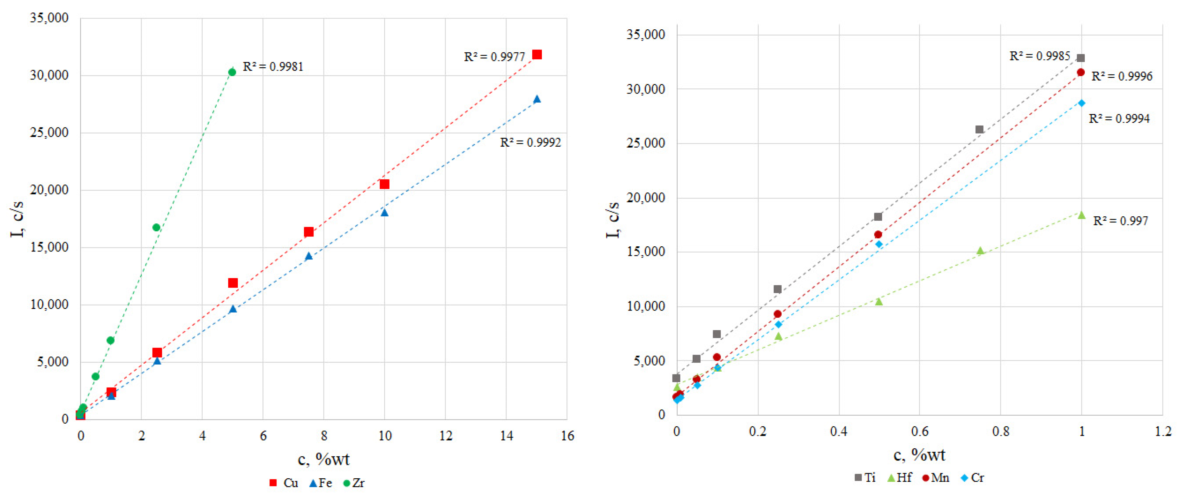
The calibration curves for waste Sm-Co magnets are shown in Figure 1. The linear correlation coefficients were not less than 0.9970. Therefore, the prepared comparison samples can be used for quantitative element determination.
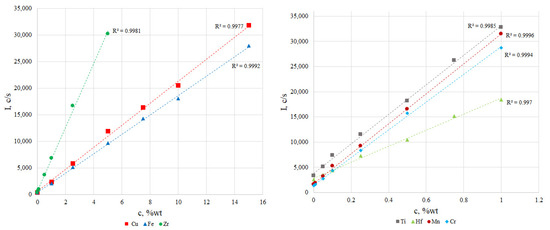
Figure 1.
Calibration curves for determined elements.
2.3. LOD and LOQ
LOD and LOQ were calculated using Equation (2) and Equation (4), respectively. They are presented in Table 2.
Table 2.
LOD и LOQ of the determination elements in waste Sm-Co magnets, wt%.
High limits for iron can be explained by the superposition of the Sm Lβ3 line on the Fe Kα line. Limits for copper may be overestimated due to the influence of hardware components (copper is included in the structure of the X-ray tube).
2.4. The Results of XRF Analysis with Calibration Curves
The results of XRF determination using calibration curves are given in Table 3, comparing ICP-OES and certified values.
Table 3.
Results of XRF determination and comparison between ICP-OES and certified values (n = 3, p = 0.95), wt%.
According to the presented data there are no significant differences between the results obtained by XRF and ICP-OES. The measurement accuracy of XRF with calibration curves was 1–2%. The proposed methods for preparing reference samples and constructing calibration dependencies allow us to simultaneously determine the main components and impurities with sufficient accuracy and acceptable sensitivity.
3. Materials and Methods
3.1. Apparatus
A SPEKTROSKAN MAX-GVM (Spectron Ltd., St. Petersburg, Russia) wavelength dispersive X-ray fluorescence spectrometer was used to perform all the measurements.
Technical parameters of spectrometer:
- determined elements—from Na to U;
- spectral resolution—crystal diffraction;
- X-ray optical scheme—according to Johansson;
- X-ray tube anode voltage—40 kV;
- X-ray tube capacity—up to 160 W;
- X-ray tube current—from 0.5 to 3.5 mA;
- X-ray tube anode—Pd;
- crystal-analyzers: single crystal of lithium fluoride LiF200, pentaerythrinol PET, rubidium biphthalate RbAP, graphite C002. The parameters of the crystal analyzers are shown in Table 4 [48].
Table 4. The parameters of the crystal analyzers.
SPECTROSCAN MAX-GVM uses a two-chamber proportional detector as a detector that converts X-ray light quanta into voltage pulses. The X-ray window is made of a beryllium film with a thickness of 15 µm; the entrance window is 12 µm thick [49].
The angle of incidence between the X-ray tube and the sample is 55° (from the center of the anode to the center of the sample with a spread in the range from 59 to 64°). The angle of reflection is 40 degrees (scatter from 35 to 45°).
The obtained spectral information was processed using the Spektr-Kvant software (the Fundamental Parameters Method and Product Graduation programs).
3.2. Waste Sm-Co Magnets Samples
The spent Sm-Co magnets considered in this study were a combined sample of several batches. The samples contained 46–61% Co, 32–39% Sm, 0.2–13% Fe, 0.01–6% Cu, 0.1–2% Zr and other impurities (Ti, Hf, Ni, Mn, Cr). The samples of spent Sm-Co magnets were an agglomeration of a monolith, chips and dispersed material.
3.3. Sample Preparation
The analysis sample in metal shaving form was thoroughly cleaned to remove mechanical contaminants (if necessary, washed with distilled water or wiped with ethanol). The material was ground using a Mecatome T210 automatic precision machine and an IV 6 vibration grinder (OOO Vibrotekhnik, St. Petersburg, Russia) [50] for 4.5 min. The particle size was no more than 50 microns. Technical parameters of vibration grinder:
- platform vibration frequency: 1500 vibrations/min;
- platform vibration amplitude: 3.5 mm;
- headset material (bowl, balls): wolfram carbide;
- headset hardness: 1180–1280 HV.
After grinding, the powders were pressed using a PLG-12 laboratory hydraulic press (Lab Tools, St. Petersburg, Russia). A total of (2 ± 0.1) g of sample was placed on a boric acid substrate. The pressing pressure was 220 bar (8.8 t).
3.4. X-ray Fluorescence Analysis Using the Method of FPM
3.4.1. Selection of Conditions for Conducting XRF-FPM
The selection of analytic lines is the most important problem in X-ray fluorescence analysis. When choosing analytical lines, it is necessary to focus on spectral interferences from matrix and impurity elements. The reveal spectral interferences to predetermine the low accuracy of XRF-FPM. It may be impossible to avoid them without iteration calculation. For example, both peaks of iron (Kα и Kβ) have spectral overlaps from matrix elements. The lines of cobalt and samarium overlap on the Fe Kβ peak, so it is impossible to obtain a pure line. At the same time, the Fe Kα line resolves with the Sm Lβ3 line although it is affected by it.
The SPECTROSCAN MAX-GVM spectrometer has four crystal analyzers with different interplanar spacings. It allows the optimization of the analysis conditions in different wavelength ranges. Generally, a crystal should be chosen on which the K-series peaks for the elements are recorded, unless they are distorted due to various effects and are not suitable for analysis. Therefore, the Kα peak on the LiF200 crystal was chosen for zirconium instead of the Lα1 line on the PET crystal. If the lines of both α-series and β-series of the same element do not have significant influences from other components, it is worth choosing the α-series, since it is characterized by the highest intensity. For example, in the case of samarium, we choose the Lα1 line, but not Lβ1.
Each analyzer crystal has 2 reflection orders. The first reflection order is usually preferred for analysis because the signal of the lines of interest is much higher than when using the second reflection order. The second reflection order is used when it is difficult or impossible to carry out an analysis using lines measured in the first reflection order or in the case of spectral overlapping. Peaks that are not resolved in the first reflection order can be resolved in the second reflection order [51]. For example, the Hf Lα1 line is present on the LiF200 crystal analyzer both in the first and the second reflection order. However, it is affected by the Cu Kα and Co Kβ1,3 peaks in the first reflection order, and Zr Kα (which appears in the spectrum from the second reflection). In the second reflection order of the LiF200 crystal, the Hf Lα1 line is not affected by these elements.
Selected lines are listed in Table 5.
Table 5.
Selected analytical lines.
The next stage of research was the selection of a measuring time for each line and tube current. The limit value of the signal for the detector of the spectrometer must be considered while selecting the analysis conditions. The main principle for choosing line measurement parameters is the following condition (for this spectrometer) [52]:
[Intensity] × [Time] = 10,000 ÷ 30,000 impulses
This limitation was chosen to avoid detector overload, which can lead to its premature failure. In addition, too high line intensity, associated with a high content of the element in the sample, makes it difficult to collect statistics due to miscalculations and, respectively, increases the uncertainty [51]. Since the intensity directly depends on the tube current, it must be increased at low intensities. In cases where the intensity of the line greatly exceeds the values (1), it is necessary to reduce the current and time or change the line. Thus, in the case of cobalt, the Kα intensity was 206,400 imp/s, while Kβ1,3 was 29,500 imp/s. In this case, it is better to choose the Co Kβ1,3 line.
The selected analysis conditions are shown in Table 6. The tube voltage did not change and was 40 kV.
Table 6.
Selected experimental conditions for XRF- FPM.
3.4.2. The XRF-FPM Experiment
Three parallel samples were taken for each probe. Pressed tablets were placed in an aluminum holder (cassette) with a hole diameter of 15 mm. The conditions for analysis are shown in Table 6. All samples were measured with the withdrawal from irradiation at least twice under repeatability conditions.
3.5. Preparation of Calibration Samples
Calibration samples were made based on the results of the samples analyzed by the fundamental parameter method (Table 1) with the composition presented in Table 7:
Table 7.
The composition of calibration samples.
Calibration sample production was based on the addition of determined elements, in the form of solutions and small dispersed powders of controlled sizes, to Sm2Co7 powder which was pure in terms of defined impurities. Further, samples were heated, ground and homogenized. This process is characterized by important advantages repeatedly confirmed by the development of reference materials of high-purity substances [53].
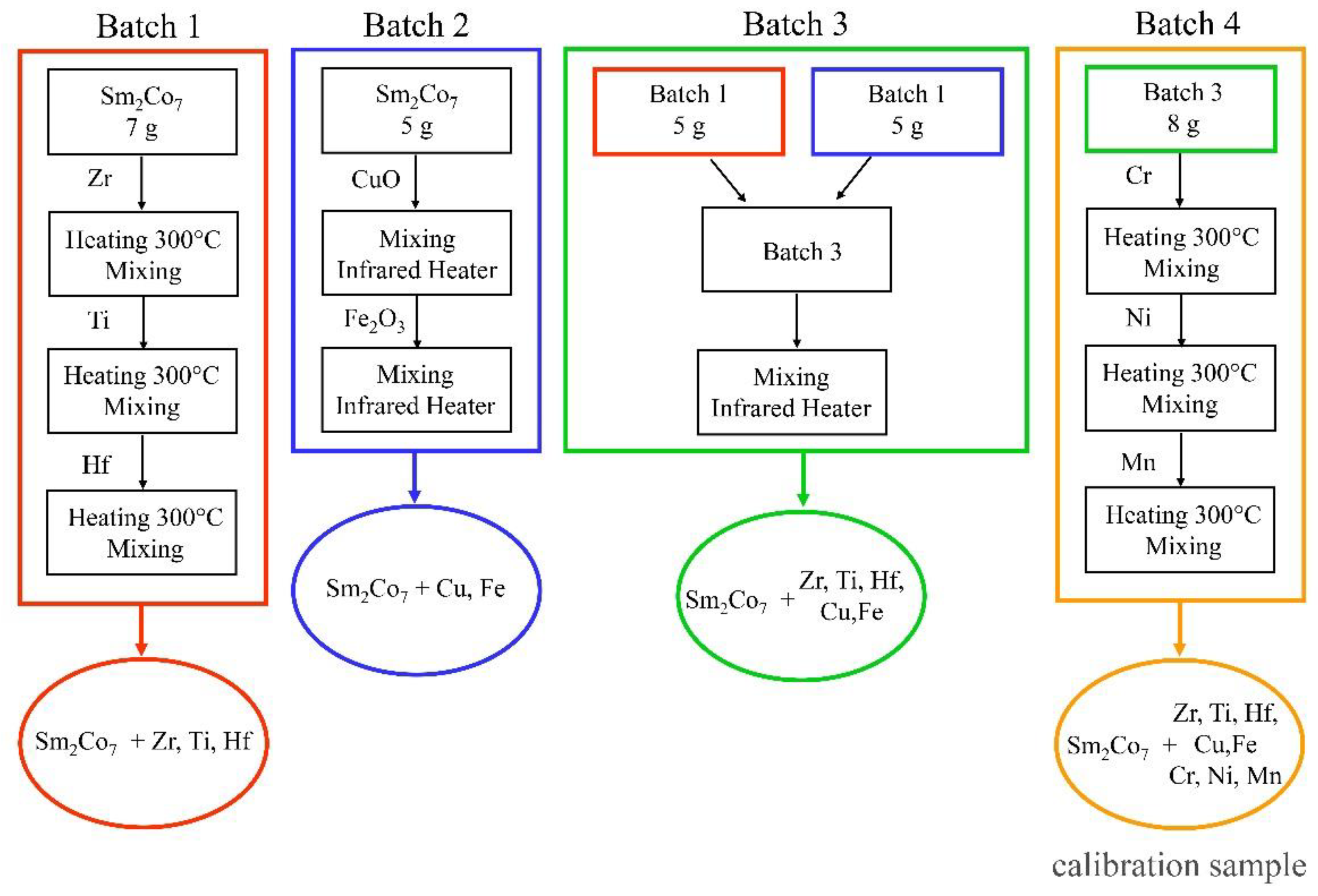
The treatment by solutions provides sufficiently high homogeneity of impurity-elements distribution. At the same time, there are practically no problems with controlling impurities imported with reagents during synthesis. Calibration sample preparation consisted of 4 steps, which resulted in 4 batches of Sm2Co7 powder with added impurities (Figure 2). The suspensions were taken using laboratory scales VL-224V (permissible measurement uncertainty 0.005–0.015 mg).
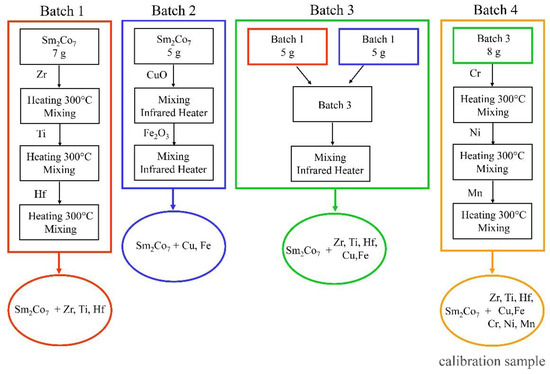
Figure 2.
Scheme for the preparation of calibration samples.
Batch 1: Single-element standards containing 10 g/L of Zr, Hf, Ti (High-Purity Standards, North Charleston, SC, USA) were sequentially applied to 7 g of Sm2Co7 powder, which was pure in terms of determined impurities (Chemcraft, Kaliningrad, Russia), in a ceramic crucible and dried in a FO-311C muffle furnace (Yamato, Tokyo, Japan) at 300 °C for one hour. The volumes of the injected standards are presented in Table 8.
Table 8.
The volume of added standard solutions and mixed powders for the preparation of calibration samples.
Batch 2: Initial Sm2Co7 powder was sequentially mixed with CuO (99.9 wt%, Chemkraft, Kaliningrad Russia) and Fe2O3 (99.999 wt%, Sigma-Aldrich, St. Louis MI, USA) powders in a graphite mortar with ethanol for 30 min and then dried for one hour in a TROMMELBERG IR 1 ECONOMY IR dryer (Trebbin, Germany). The mixing proportions of the powders are listed in Table 8.
Batch 3: A 5 g of batch 1 powder and a 5 g of batch 2 powder were mixed in a graphite mortar with ethanol for 30 min, then dried for one hour using IR drying.
Batch 4: Single element standard solutions containing 10 g/L of Mn, Ni, Cr (High-Purity Standards, North Charleston, SC, USA) were sequentially applied on 8 g of powder from batch 3 and dried in a muffle furnace at 300 °C for one hour. The volumes of the injected standards are demonstrated in Table 8.
Batch 4 was used to plot the calibration curves. The process was repeated for the preparation of each calibration sample (CS2–CS7). The composition of the obtained samples was confirmed by ICP-OES.
3.6. Quantitative XRF Analysis Using Calibration Curves
Three replicate samples were prepared for analysis: both for calibration samples and for test samples. Prepared pressed tablets of calibration and test samples were placed in an aluminum holder with a hole diameter of 15 mm. Intensities were measured under the conditions and modes of operation presented in Table 9. To establish the calibration characteristic, the analytical signal for each determined element in every batch sample was measured with the withdrawal from irradiation at least twice under repeatability conditions.
Table 9.
Selected experimental conditions for quantitative XRF analysis. The tube voltage did not change and was 40 kV.
The selection of conditions depends on the height of the analyte’s signals. Too strong intensities (more than 30,000–40,000 impulses per second for this spectrometer) lead to detector miscalculations and peak distortion. For Sm, Co, Fe, and Cu, the lines were chosen in the second reflection order of the C002 crystal analyzer where there are slightly lower intensities. It is better to set low current values (0.2 mA) and a measuring time of 40 s for these lines to collect statistics. This decreases the standard uncertainty of calibration and leads to more accurate calibration curves. In the case of low impurity levels, it is recommended to increase the current (3.5 mA) and the measuring time (50 s) to raise the sensitivity. The line chosen for the titanium determination is sufficiently intense; therefore, an exposure time of 40 s and a tube current of 0.5 mA were chosen.
3.7. Limits of Detection (LOD) and Limits of Quantification (LOQ)
LODs were calculated using the following equation [54]:
where sb is the standard deviation of measuring the background, Δc/ΔI is reciprocal sensitivity, Ibi–background intensity value in each measurement and n–number of measurements.
LOQs were determined using equation [55]:
Measurements were performed according to the conditions given in Table 9. The number of measurements of background and analyte signals is n = 10. The data collection time is 20 s.
3.8. Comparative ICP-OES Analysis
The results obtained using the XRF method were confirmed with ICP-OES. For ICP-OES analysis, a (0.1 ± 0.005) g portion of waste was accurately measured and placed into a disposable test tube. The sample was dissolved in 2.5 mL of HNO3 at 90–110 °C for 10 min. After cooling, the solution was brought up to 100 mL with deionized water. An ICAP PRO XP spectrometer (Thermo Electron Corp., Waltham, MA, USA) was used for analysis. Operating parameters for the atomic emission spectrometer are presented in [24]. One-element ICP-OES calibration solutions from High-Purity Standards (North Charleston, SC, USA) were used to plot the calibration curves.
4. Conclusions
Analytical control of waste magnetic materials based on Sm and Co proves to be challenging and non-conventional. In this study, the capabilities of a semi-quantitative X-ray fluorescence analysis using a fundamental parameters method and approach to plot a calibration curve were shown. For the first time, the problem of calibration-sample preparation for the solid-phase X-ray fluorescence analysis for non-stereotyped objects has been solved. The linear correlation coefficients of such calibration curves were not less than 0.9970, which allowed us to use them to determine the main components and impurities. Limits of detection and limits of quantification were established for target analytes. The limits of determination were 0.0641 wt% for Fe, 0.0485 wt% for Cu, 0.0033 wt% for Zr, 0.1755 wt% for Hf, 0.0092 wt% for Ti, 0.0040 wt% for Mn, 0.082 wt% for Ni and 0.0073 wt% for Cr. The results were compared with ICP-OES and no significant differences were observed. As a result, a two-stage method for X-ray spectral analysis of waste Sm-Co magnets was developed, including a semi-quantitative variant for assessing the content of their components and their exact quantitative determination with calibration curves. By employing this approach, it becomes possible to carry out real-time quality control of solid magnetic wastes, and to choose an optimal processing scheme for these unconventional samples.
Author Contributions
Conceptualization, A.A.A., G.E.M. and V.B.B.; methodology, G.E.M.; software, M.S.D. and N.A.K.; validation, G.E.M. and M.S.D.; formal analysis, A.A.A. and N.A.K.; investigation, A.A.A. and G.E.M.; resources, V.B.B.; data curation, M.S.D. and V.B.B.; writing—original draft preparation, A.A.A. and G.E.M.; writing—review and editing, M.S.D. and V.B.B.; visualization, A.A.A. and N.A.K.; supervision, V.B.B.; project administration, M.S.D. and V.B.B.; funding acquisition, V.B.B. All authors have read and agreed to the published version of the manuscript.
Funding
This work was supported by the Ministry of Science and Higher Education of Russia (Grant Agreement №075-15-2020-782).
Data Availability Statement
All data used to support the findings of this study are included within the article.
Acknowledgments
This research was performed using equipment from the JRC PMR IGIC RAS.
Conflicts of Interest
The authors declare no conflict of interest.
References
- Strnat, K.; Hoffer, G.; Olson, J.; Ostertag, W.; Becker, J.J. A family of new cobalt-base permanent magnet materials. J. Appl. Phys. 1967, 38, 1001–1002. [Google Scholar] [CrossRef]
- Gutfeisch, O.; Willard, M.A.; Bruck, E.; Chen, C.H.; Sankar, S.G.; Liu, J.P. Magnetic materials and devices for the 21st century: Stronger, lighter, and more energy efficient. Adv. Mater. 2011, 23, 821–842. [Google Scholar] [CrossRef] [PubMed]
- Zhou, X.; Huang, A.; Cui, B.; Sutherland, J.W. Techno-Economic Assessment of a Novel SmCo Permanent Magnet Manufacturing Method. Procedia CIRP 2021, 98, 127–132. [Google Scholar] [CrossRef]
- Binnemans, K.; Jones, P.T.; Blanpain, B.; Gerven, T.V.; Yang, Y.X.; Walton, A.; Buchert, M. Recycling of rare earths: A critical review. J. Clean. Prod. 2013, 51, 1–22. [Google Scholar] [CrossRef]
- Yi, J.H. Development of samarium–cobalt rare earth permanent magnetic materials. Rare Met. 2014, 33, 633–640. [Google Scholar] [CrossRef]
- Gong, Y.; Qiu, Z.; Liang, S.; Zheng, X.; Meng, H.; Zheng, Z.; Chen, D.; Yuan, S.; Xia, W.; Zeng, D.; et al. Strategy of preparing SmCo based films with high coercivity and remanence ratio achieved by temperature and chemical optimization. J. Rare Earths 2023. [Google Scholar] [CrossRef]
- Coey, J.M.D. Perspective and Prospects for Rare Earth Permanent Magnets. Engineering 2020, 6, 119–131. [Google Scholar] [CrossRef]
- Chen, B.; Li, L.; Zhu, S.; Zhang, W.; Gao, Z. Excellent magnetic and mechanical properties of the Sm2Co17-based magnets fabricated via microwave processing. J. Alloys Compd. 2021, 868, 159071. [Google Scholar] [CrossRef]
- Sun, W.; Zhu, M.; Fang, Y.; Liu, Z.; Chen, H.; Guo, Z.; Li, W. Magnetic properties and microstructures of high-performance Sm2Co17 based alloy. J. Magn. Magn. Mater. 2015, 378, 214–216. [Google Scholar] [CrossRef]
- Chen, C.H.; Walmer, M.S.; Walmer, M.H.; Liu, S.; Kuhl, E.; Simon, G. Sm-2(Co, Fe, Cu, Zr)(17) magnets for use at temperature ⩾ 400 °C. J. Appl. Phys. 1998, 83, 6706–6708. [Google Scholar] [CrossRef]
- Sinha, M.K.; Pramanik, S.; Kumari, A.; Sahu, S.K.; Prasad, L.B.; Jha, M.K.; Yoo, K.; Pandey, B.D. Recovery of value added products of Sm and Co from waste SmCo magnet by hydrometallurgical route. Sep. Purif. Technol. 2017, 179, 1–12. [Google Scholar] [CrossRef]
- Tanaka, M.; Oki, T.; Koyama, K.; Narita, H.; Oishi, T. Chapter 255—Recycling of Rare Earths from Scrap. In Handbook on the Physics and Chemistry of Rare Earths; Jean-Claude, G.B., Vitalij, K.P., Eds.; Elsevier: Amsterdam, The Netherlands, 2013; Volume 43, pp. 159–211. [Google Scholar] [CrossRef]
- Lorenz, T.; Bertau, M. Recycling of rare earth elements from SmCo5-Magnets via solid-state chlorination. J. Clean. Prod. 2020, 246, 118980. [Google Scholar] [CrossRef]
- Binnemans, K.; Jones, P.T.; Müller, T.; Yurramendi, L. Rare earths and the balance problem: How to deal with changing markets? J. Sustain. Metall. 2018, 8, 126–146. [Google Scholar] [CrossRef]
- Ullmann, F. Encyclopedia of Industrial Chemistry; Wiley: Hoboken, NJ, USA, 2013. [Google Scholar] [CrossRef]
- Coey, J.M.D. Permanent magnet applications guide. J. Magn. Magn. Mater. 2002, 248, 441–456. [Google Scholar] [CrossRef]
- Xu, X.; Khoshima, S.; Karajic, M.; Balderman, J.; Markovic, K.; Scancar, J.; Rozman, K.Z. Electrochemical routes for environmentally friendly recycling of rare-earth-based (Sm–Co) permanent magnets. J. Appl. Electrochem. 2022, 52, 1081–1090. [Google Scholar] [CrossRef]
- An, S.; Li, X.; Li, W.; Ren, F.; Xu, P. Coercivity enhancement of SmCo/FeCo nanocomposite magnets by doping eutectic Sm-Zn alloy. Mater. Lett. 2021, 284, 128965. [Google Scholar] [CrossRef]
- Kuchumov, V.A.; Shoomkin, S.S. Analisys of the chemichal composition of the bearing alloy used in the production of Sm-Co-based permanent magnets. St. Petersburg Polytech. Univ. J. Eng. Sci. Technol. 2017, 23, 219–225. [Google Scholar] [CrossRef]
- Shumkin, S.S.; Prokof’ev, P.A.; Semenov, M.Y. Production of permanent magnets for magnetically hard alloys using rare-earth metals. Metallurgist 2019, 63, 462–468. [Google Scholar] [CrossRef]
- Yang, Q.; Liu, Z.; Gao, X.; Wu, H.; Zhu, C.; Cheng, W.; Ma, Y.; Chen, R.; Yan, A. Prolonged ordering process induced higher segregation of copper in 2:17 type SmCo magnets. J. Alloys Compd. 2022, 924, 166463. [Google Scholar] [CrossRef]
- Teng, Y.; Li, Y.; Xu, X.; Yue, M.; Liu, W.; Zhang, D.; Zhang, H.; Lu, Q.; Xia, W. Microstructure evolution of hot-deformed SmCo-based nanocomposites induced by thermo-mechanical processing. J. Mater. Sci. Technol. 2023, 138, 193–202. [Google Scholar] [CrossRef]
- Petrova, K.V.; Baranovskaya, V.B.; Korotkova, N.A. Direct inductively coupled plasma optical emission spectrometry for analysis of waste samarium-cobalt magnets. Arab. J. Chem. 2022, 15, 103501. [Google Scholar] [CrossRef]
- Renko, M.; Osojnik, A.; Hudnik, V. ICP emission spectrometric analysis of rare earth elements in permanent magnet alloys. Fresenius J. Anal. Chem. 1995, 351, 610–613. [Google Scholar] [CrossRef]
- Iwasaki, K.; Uchida, H. Rapid Determination of Major and Minor Elements in Rare Earth-Cobalt Magnets by Inductively Coupled Plasma Atomic Emission Spectrometry. Anal. Sci. 1986, 2, 261–264. [Google Scholar] [CrossRef]
- Orefice, M.; Audoor, H.; Li, Z.; Binnemans, K. Solvometallurgical route for the recovery of Sm, Co, Cu and Fe from SmCo permanent magnets. Sep. Purif. Technol. 2019, 219, 281–289. [Google Scholar] [CrossRef]
- Korotkova, N.A.; Baranovskaya, V.B.; Petrova, K.V. Microwave Digestion and ICP-MS Determination of Major and Trace Elements in Waste Sm-Co Magnets. Metals 2022, 12, 1308. [Google Scholar] [CrossRef]
- Akin, H.; Emre, C.M.; Topcuoglu, T.; Kemal Ozdemir, A. Can laser welding stop corrosion of new generation magnetic attachment systems. Mater. Res. Innov. 2011, 15, 66–69. [Google Scholar] [CrossRef]
- Matthews, M.W.; Eggleston, H.C.; Pekarek, S.D.; Hilmas, G.E. Magnetically adjustable intraocular lens. J. Cataract Refract. Surg. 2003, 29, 2211–2216. [Google Scholar] [CrossRef]
- Sherman, J.; Winifred, J.M. Adjustment of an Inverse Matrix Corresponding to Changes in the Elements of a Given Column or a Given Row of the Original Matrix. Ann. Math. Stat. 1950, 21, 124–127. [Google Scholar] [CrossRef]
- Bondarenko, A.V.; Belonovsky, A.V.; Katzman, Y.M. Application of fundamental parameter method in X-ray fluorescence Analysis of Pulp Products in Ore Concentration. Gorn. Prom. 2021, 5, 84–88. [Google Scholar]
- Beckhoff, B.; Kanngießer, B.; Langhoff, N.; Wedell, R.; Wolff, H. Handbook of Practical X-ray Fluorescence Analysis; Part 5 Quantitative Analysis; Springer: Berlin/Heidelberg, Germany, 2006. [Google Scholar]
- Borkhodoev, V.Y. X-ray Fluorescence Analysis of Rocks by the Method of Fundamental Parameters; SVKNII FEB RAN: Magadan, Russia, 1999; 279p. [Google Scholar]
- Coulthard, I.; Freeland, J.W.; Winarski, R.; Ederer, D.L.; Jiang, J.S.; Inomata, A.; Bader, S.D.; Callcott, T.A. Soft x-ray absorption of a buried SmCo film utilizing substrate fluorescence detection. Appl. Phys. Lett. 1999, 74, 3806–3808. [Google Scholar] [CrossRef]
- Itza-Ortiz, V.; Ederer, D.L.; Schuler, T.M.; Ruzycki, N.; Samuel Jiang, J.; Bader, S.D. Model study of soft x-ray spectroscopy techniques for observing magnetic circular dichroism in buried SmCo magnetic films. J. Appl. Phys. 2003, 93, 2002–2008. [Google Scholar] [CrossRef]
- Foltova, S.S.; Hoogerstraete, T.V.; Banerjee, D.; Binnemans, K. Samarium/cobalt separation by solvent extraction with undiluted quaternary ammonium ionic liquids. Sep. Purif. Technol. 2019, 210, 209–218. [Google Scholar] [CrossRef]
- Rabenberg, L.; Mishra, R.; Thomas, G. Microstructures of Precipitation Hardened SmCo Permanent Magnets; LBNL Report #: LBL-13395; Lawrence Berkeley National Laboratory: Berkeley, CA, USA, 1981. [Google Scholar]
- Chen, D.K.; Luo, L.; Dai, F.L.; Liu, P.P.; Yao, Q.R.; Wang, J.; Zhou, H.Y. Phase Equilibria in Sm-Co-Ti Ternary System. J. Phase Equilib. Diffus. 2022, 43, 317–331. [Google Scholar] [CrossRef]
- Shumkin, S.S.; Sitnov, V.V.; Kamynin, A.V.; Chernyshov, B.D.; Semenov, M.Y.; Nikolaichik, V.I. Composition and Operating Properties of Hard Magnetic Materials Based on Alloys of the Sm–Co–Cu–Fe–Zr System Obtained with the Use of Recoverable Resources. Met. Sci. Heat Treat. 2022, 63, 479–485. [Google Scholar] [CrossRef]
- Cadieu, F.J.; Vander, I.; Rong, Y.; Zuneska, R.W. Glancing XRD and XRF for the study of texture development in SmCo based films sputtered onto silicon substrates. Adv. X-ray Anal. 2011, 55, 162–176. [Google Scholar]
- Gómez, E.; Cojocaru, P.; Magagnin, L.; Valles, E. Electrodeposition of Co, Sm and SmCo from a deep eutectic solvent. J. Electroanal. Chem. 2011, 658, 18–24. [Google Scholar] [CrossRef]
- Swain, N.; Mishra, S.; Acharya, M.R. Hydrometallurgical route for recovery and separation of samarium (III) and cobalt (II) from simulated waste solution using tri-n-octyl phosphine oxide—A novel pathway for synthesis of samarium and cobalt oxides nanoparticles. J. Alloys Compd. 2020, 815, 152423. [Google Scholar] [CrossRef]
- Allocca, L.; Bonavolontà, C.; Giardini, A.; Lopizzo, T.; Morone, A.; Valentino, M.; Verrastro, M.F.; Viggiano, V. Laser deposition of SmCo thin film and coating on different substrates. Phys. Scr. 2008, 78, 058114. [Google Scholar] [CrossRef]
- Allocca, L.; Gambardella, U.; Morone, A.; Valentino, M. Laser deposition of SmCo thin film on steel substrate. In Proceedings of the SPIE 6985, Fundamentals of Laser Assisted Micro- and Nanotechnologies, St. Petersburg, Russian, 24 January 2008; p. 69850. [Google Scholar] [CrossRef]
- Morone, M.V.; Annunziata, F.D.; Giugliano, R.; Chianese, A.; De Filippis, A.; Rinaldi, L.; Gambardella, U.; Franci, G.; Galdiero, M.; Morone, A. Pulsed laser ablation of magnetic nanoparticles as a novel antibacterial strategy against gram positive bacteria. Appl. Surf. Sci. Adv. 2022, 7, 100213. [Google Scholar] [CrossRef]
- Ono, K.; Kakefuda, Y.; Okuda, R.; Ishii, Y.; Kamimura, S.; Kitamura, A.; Oshima, M. Organometallic synthesis and magnetic properties of ferromagnetic Sm–Co nanoclusters. J. Appl. Phys. 2002, 91, 8480–8482. [Google Scholar] [CrossRef]
- Vander, I.; Zuneska, R.; Cadieu, F. Thickness determination of SmCo films on silicon substrates utilizing X-ray diffraction. Powder Diffr. 2010, 25, 149–153. [Google Scholar] [CrossRef]
- Mazurickij, M.I. X-ray Spectral Optics: Educational Materials for Lectures and Practical Classes/M.I. Mazurickij; Diapazon: Rostov-na-Donu, Russia, 2005; p. 91s. [Google Scholar]
- Mishin, V.V.; Shishov, I.A.; Kiselev, P.P.; Matsinkevich, E.V.; Rudnev, A.V.; Bukin, K.V. Investigation of the possibility of improving the X-ray fluorescence spectrometer analytical characteristics due to using the superfine beryllium foils. Mater. Phys. Mech. 2018, 36, 92–99. [Google Scholar] [CrossRef]
- Krivelev, D.M. Vibration Grinder. RU Patent 2018137072, 15 January 2019. [Google Scholar]
- Shirkin, L.A. X-ray fluorescent analysis of environmental objects. In Tutorial; Publishing House VLSU: Vladimir, Russia, 2009; 65p. [Google Scholar]
- Kalinin, B.D. Expanding the Analytical Capabilities of X-ray Fluorescence Analysis on the Principles of Theoretical Corrections of Interelement Influences. Ph.D. Thesis, St. Petersburg University, Saint Petersburg, Russia, 2008; pp. 342p. (In Russian). [Google Scholar]
- Lisienko, D.G.; Dombrovskaya, M.A.; Muzgin, V.N. Problems of development of standard samples of the composition of pure materials, attested by the calculation method. Meas. Equip. 1999, 10, 66–67. [Google Scholar]
- Borkhodoev, V.Y. About a correlation between the limits of detection and determination in X-ray fluorescence analysis. J. Anal. Chem. 2015, 70, 1307–1312. [Google Scholar] [CrossRef]
- Thomsen, V.; Schatzlein, D.; Mercuro, D. Limits of Detection in Spectroscopy. Spectroscopy 2003, 18, 112–114. [Google Scholar]
Disclaimer/Publisher’s Note: The statements, opinions and data contained in all publications are solely those of the individual author(s) and contributor(s) and not of MDPI and/or the editor(s). MDPI and/or the editor(s) disclaim responsibility for any injury to people or property resulting from any ideas, methods, instructions or products referred to in the content. |
© 2023 by the authors. Licensee MDPI, Basel, Switzerland. This article is an open access article distributed under the terms and conditions of the Creative Commons Attribution (CC BY) license (https://creativecommons.org/licenses/by/4.0/).