Environmental Sustainability of Niobium Recycling: The Case of the Automotive Industry

Abstract

The recycling of scrap is one of the common approaches aiming at reduction of mining-based production of critical metals and mitigation of their supply risk as well as processing-related environmental impact. The number of currently available end-of-life vehicles (ELVs) indicates—significant potential for critical metals recycling, especially niobium (Nb). Therefore, the quantification of environmental impact of niobium recovery starts to be an important issue in assessment of sustainability of large-scale recycling processes. In this paper, we assess energy consumption and greenhouse gas (GHG) emissions in individual stages of niobium supply chain in the automotive industry over the period 2010–2050. The different stages including mining, production and recycling are analyzed using dynamic simulation. The results show the majority of the consumed energy (45% of energy demand in niobium supply chain) is used in the primary production stage. This stage also contributes to 72% of total gas emissions of supply chain over the period 2010–2050. Mining of niobium consumes up to 36% of energy and generates ca. 21% of GHG emissions. While, in recycling stage, the secondary production of niobium requires 19% of supply chain energy and generates 7% of gas emissions. The detailed calculations show that recycling of niobium could save around 133–161 m GJ energy between 2010 and 2050. The recycling would also contribute to the reduction of 44–53 mt CO₂-eq in the same period. It shows around 18% reduction of annual emissions between 2010 and 2050 thanks to reuse of niobium in secondary production rather than primary production.

1. Introduction

Niobium (Nb) is an essential element for production of steel and superalloys, superconductors, electronic components, medical implants, etc. The estimated resources of niobium are substantial and they are sufficient to meet the worldwide demand in the foreseeable future [1]. However, the oligopoly nature of the niobium market and the lack of substitutes create its supply risk [2,3,4,5]. It is worth to mention that the niobium demand has increased dramatically over the past decade, particularly as an element of microalloys in high strength and stainless steels used in the automotive industry [6].

The global market of niobium grew annually by 10% between 2000 and 2010 [7]. In view of the rapid increase in primary and secondary niobium production over the last 15 years [8], the production rate will peak in 2025 with recycling rate at around 60% [9]. Therefore, the most significant increase in demand for niobium will take place in the coming years.

In the production of steel for the automotive industry, Nb is used in the form of ferroniobium. Ferroniobium represents the most significant fraction of the world’s demand of niobium—around 87% [1]. The growing use of ferroniobium in the automotive industry is driven by a trend to reduce the weight of the vehicles [10,11,12].

The end-of-life vehicles (ELVs) have become a major waste stream [13]. Therefore, maximisation of recyclability is one of the dominant trends in car manufacturing. It can contribute considerably to the reduction of the wastes but also constitutes a significant source of raw materials. For example, in 2010, the total number of ELVs was around 40 million; mainly in Germany, Italy, France, UK, Spain, USA, Canada, Brazil, Japan, China, Korea and Australia [14]. On average concentration of Nb in steel alloy is low and generally lower than 0.1 wt% [1]. However, a considerable number of ELVs makes this source of niobium quite important. In 2010, based on the available global number of ELVs, the amount of niobium in high-strength steel (HSS) alloy used in passenger cars (average weight 1.5 tonnes) could be estimated at around 36,000 tonnes compared to 49,100 tonnes of niobium mined globally [15]. The annual global production of niobium alloyed steel was estimated at about 50 million tonnes [16]. According to the estimates provided by the automotive industry for 2020, the steel content in a typical car will increase from 54% to 64% [17].

The decision makers need to be aware of possible environmental effects at each stage of the supply chain when analysing the use of virgin ores or recycled materials [18]. In the automotive industry, recycling strategies for critical materials in ELVs are poorly understood due to the complexity of the material flows [19] as well as environmental and economic implications of critical materials recycling [20].

In recent decades, supply chain research has attempted to address the issues of environmental impact and social sustainability [21,22,23]. Moreover, new avenues of research have been opened to aim at developing holistic perspectives of sustainability of supply chain. From this perspective, researchers have started investigating the available options for reaching both higher economic growth and lower GHG emissions [24,25]. In this case, the effect of energy consumption on sustainability and its impact on GHG emissions are very important issues relevant in all stages of the supply chain [26,27]. However, the question remains as to what levels of energy consumption and GHG emissions at each stage of the niobium supply chain would ensure environmental sustainability. Therefore, the main objective of this paper is to present a dynamic model of the niobium supply chain to investigate energy consumption and GHG emissions at each stage including mining, production and recycling.

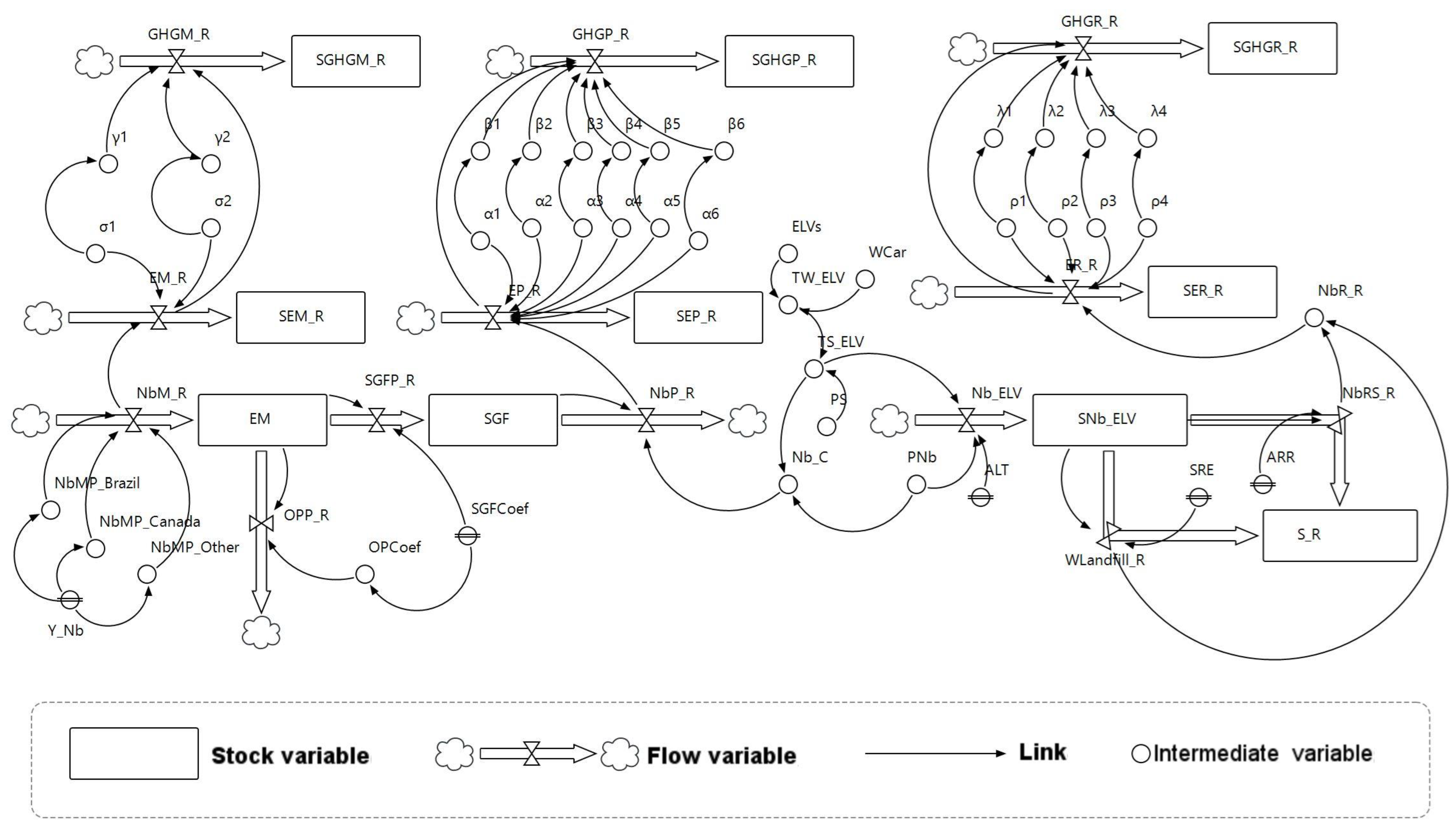
2. Dynamic Model of Niobium Supply Chain

The assessment of specific modifications of supply chain needs a systems approach. It consists of the detailed analysis of dynamics of all stages of the supply chain [12]. Therefore, the methodology of system dynamics introduced by Forrester [28] is used in this study. The system dynamics methodology has been used in many applications, both in social sciences and engineering. In the case of critical materials, system dynamics models have been used in different sectors for such materials as indium [29], platinum group metals [30], rare earth elements [31], uranium [32], lithium [33], phosphorus [34] and niobium [35].

The model presented in this paper considers the complex interrelationships between mining and processing, production and recycling stages of niobium global supply chain. In production stage, we consider niobium manufacturing in the automotive industry. The structural model is built and simulated by identifying the key variables and their interactions in the different stages of niobium life cycle. The conceptual model is presented in Figure 1, where niobium flow starts with the mining stage and next the interrelations with other stages are considered. Each stage of the model consists of three main layers (submodels), including material and energy flow as well as GHG emissions. The first submodel, material flow, is composed of the following modules: mining, extraction, processing, production, consumption, collection and recycling. The energy consumption submodel takes into account energy consumed in mining, production and recycling. The GHG emissions submodel is primarily related to the energy consumption and therefore the structure of both submodels are identical. There was analyzed flow of niobium in the different processes, e.g., pyrochlore ore extraction, ferroniobium production, standard grade ferroniobium production, HSS steel production for automobile industry, ELVs collection process and recycling of HSS steel. Therefore, there were assessed energy consumption and GHG emissions of those processes. Below, we present the analysis of the particular stages in detail.

System Definition and Model Description

Figure 2 shows the simulation model. In system dynamics modeling, state variables change continuously over time. System dynamics model is a complex system incorporating three types of variables: (i) stock (or level) variable that is a reservoir of a given resource (also called state variable), (ii) flow variable that adjusts the level of stock through inbound and outbound flows, and (iii) intermediate variable (auxiliary) consisting of functions of stocks (and constants or exogenous inputs) [36]. It is important to note that every variable in system dynamics model is calculated at each time step. For example, in this work, we consider time step equal to one year as the used input data are based on yearly reports. In this study, data are collected from different sources for time horizon 1950–2017 (Appendix,

Table A1. Data sources for all inputs of the proposed model.

Variable/Parameter	Description	Unit	Value Range	Time	Data Sources
NbMP-Brazil (t)	World production of mineral concentrates (niobium content) by Brazil	Tonnes	21,800–101,022	2000–2015	US Geological Survey (USGS). Available at: https://minerals.usgs.gov/minerals/pubs/commodity/niobium/
NbMP-Canada (t)	World production of mineral concentrates (niobium content) by Canada	Tonnes	2280–5774	2000–2015	US Geological Survey (USGS). Available at: https://minerals.usgs.gov/minerals/pubs/commodity/niobium/
NbMP-Other (t)	World production of mineral concentrates (niobium content) by other countries	Tonnes	89–853	2000–2015	US Geological Survey (USGS). Available at: https://minerals.usgs.gov/minerals/pubs/commodity/niobium/
RBrazil (t)	Reserves in Brazil	Tonnes	3,300,000–4,100,000	1996–2017	US Geological Survey (USGS). Available at: https://minerals.usgs.gov/minerals/pubs/commodity/niobium/niobimcs96.pdf https://minerals.usgs.gov/minerals/pubs/commodity/niobium/mcs-2017-niobi.pdf
RCanada (t)	Reserves in Canada	Tonnes	140,000–200,000	1996–2017	US Geological Survey (USGS). Available at: https://minerals.usgs.gov/minerals/pubs/commodity/niobium/niobimcs96.pdf https://minerals.usgs.gov/minerals/pubs/commodity/niobium/mcs-2017-niobi.pdf
C1-Brazil (t)	One of the leading niobium ore and concentrate producers: Companhia Brasileira de Metalurgia e Mineração (CBMM) in Brazil	Tonnes	19,500–150,000	1991–2016	US Geological Survey (USGS). Available at: https://minerals.usgs.gov/minerals/pubs/commodity/niobium/230494.pdf https://minerals.usgs.gov/minerals/pubs/commodity/niobium/myb1-2014-niobi.pdf
CCanada (t)	One of the leading niobium ore and concentrate producers: IAMGOLD Corporation (Niobec Mine) in Canada	Tonnes	3300–5480	1994–2014	US Geological Survey (USGS). Available at: https://minerals.usgs.gov/minerals/pubs/commodity/niobium/230494.pdf https://minerals.usgs.gov/minerals/pubs/commodity/niobium/myb1-2014-niobi.pdf
C2-Brazil (t)	One of the leading niobium ore and concentrate producers: Mineração Catalão de Goias in Brazil	Tonnes	3550–4700	1995–2014	US Geological Survey (USGS). Available at: https://minerals.usgs.gov/minerals/pubs/commodity/niobium/230495.pdf https://minerals.usgs.gov/minerals/pubs/commodity/niobium/myb1-2014-niobi.pdf
SGFCoef	Percentage of global niobium production used to produce ferroniobium used in high strength low alloy steels	%	0.89	2011	British Geological Survey’s Centre for Sustainable Mineral Development MineralsUK. Mineral Profiles. Niobium and Tantalum. Available at: http://www.bgs.ac.uk/downloads/start.cfm?id=2033
OPCoef	Percentage of global niobium production used in manufacture of niobium alloys, niobium chemicals and carbides, high purity ferroniobium, and other niobium metal products	%	0.11	2011	British Geological Survey’s Centre for Sustainable Mineral Development MineralsUK. Mineral Profiles. Niobium and Tantalum. Available at: http://www.bgs.ac.uk/downloads/start.cfm?id=2033
δ1	Energy usage through hydrofluoric acid dissolution process	GJ (tonne ore)−1	2	2003	National Institute of Materials Science (estimation of CO2 emission and energy consumption in extraction of metals) http://www.nims.go.jp/genso/0ej00700000039eq-att/0ej00700000039j5.pdf
δ2	Energy usage through solvent extraction process	GJ (tonne ore)−1	31.4	2003	National Institute of Materials Science (estimation of CO2 emission and energy consumption in extraction of metals) http://www.nims.go.jp/genso/0ej00700000039eq-att/0ej00700000039j5.pdf
γ1	CO2 emission through hydrofluoric acid dissolution process	CO2-eq.	1.8	2003	National Institute of Materials Science (estimation of CO2 emission and energy consumption in extraction of metals) http://www.nims.go.jp/genso/0ej00700000039eq-att/0ej00700000039j5.pdf
γ2	CO2 emission through solvent extraction process	CO2-eq.	4.6	2003	National Institute of Materials Science (estimation of CO2 emission and energy consumption in extraction of metals) http://www.nims.go.jp/genso/0ej00700000039eq-att/0ej00700000039j5.pdf
PNb	Nb grade in HSS ferroniobium applied in automobiles	%	0.04–0.08, 0.1	2011–2017	[1,55] PROMETIA, Factsheet available at: http://prometia.eu/wp-content/uploads/2014/02/NIOBIUM-TANTALUM-v02.pdf
PS	Steel in Automobile	%	61.7	2012	[56]
WCar	Weight of Car	Tonne	1.11361–1.49131	1950–2010	[12]
ELVnumber (t)	End-of-life vehicles (ELV) including countries: European Union, Germany, Italy, France, England, Spain, Russian Federation, USA, Canada, Brazil, Japan, China, Korea, and Australia	Units year−1	European Union:7,823,211 Germany:500,193 Italy:1,610,137 France:1,583,283 England:1,157,438 Spain:839,637 USA:12,000,000 Canada:1,200,000 Brazil:1,000,000 Japan:2,960,000 China:3,506,000 Korea:684,000 Australia:500,000 Global total:40,176,051	2010	[14]
ALT	Automobile Average Life Time (Average Vehicle Age)	Year	16	2007–2014	[12,49,50,57]
α1	The amount of energy required in cold rolling process	GJ tonne−1	1.63–1.935	1999–2012	[12,58]
α2	The amount of energy required in hot rolling process	GJ tonne−1	1.7–1.88	1999–2012	[12,58,59,60]
α3	The amount of energy required in continuous casting process	GJ tonne−1	0.076	1999–2012	[12]
α4	The amount of energy required in basic oxygen furnace process	GJ tonne−1	0.4	1999–2012	[12,59]
α5	The amount of energy required in blast furnace process	GJ tonne−1	12.3–16	1999–2012	[12,59,60]
α6	The amount of energy required in sintering/coking process	GJ tonne−1	43.8	1999–2012	[12,61]
β1	The greenhouse gas emitted in cold rolling process	Tonne CO2-eq.	0.008	2013	[12,60]
β2	The greenhouse gas emitted in hot rolling process	Tonne CO2-eq.	0.082	2013	[12,60]
β3	The greenhouse gas emitted in continuous casting process	Tonne CO2-eq.	0	2013	[12,60]
β4	The greenhouse gas emitted in basic oxygen furnace process	Tonne CO2-eq.	0.09	1999–2012	[12,61,62]
β5	The greenhouse gas emitted in blast furnace process	Tonne CO2-eq.	1.22–1.46	1999–2012	[12,60,61,62]
β6	The greenhouse gas emitted in sintering/coking process	Tonne CO2-eq.	0.43	1999–2012	[12]
ARR	Automobile Recycling Rate	%	85	1998–2013	US Geological Survey (USGS). Flow Studies for Recycling Metal Commodities in the United States. Available at: https://pubs.usgs.gov/circ/2004/1196am/c1196a-m_v2.pdf ISRI. Available at: http://www.isri.org/docs/default-source/recycling-industry/fact-sheet---iron-and-steel.pdf?sfvrsn=16
SRE	Automobile Scrap recycling efficiency	%	50	1998	US Geological Survey (USGS). Flow Studies for Recycling Metal Commodities in the United States. Available at: https://pubs.usgs.gov/circ/2004/1196am/c1196a-m_v2.pdf
ρ1	The amount of energy required in cold rolling process for secondary production	GJ tonne−1	1.63–1.935	1999–2012	[12,58]
ρ2	The amount of energy required in hot rolling process for secondary production	GJ tonne−1	1.7–1.88	1999–2012	[12,58,59,60]
ρ3	The amount of energy required in continuous casting process for secondary production	GJ tonne−1	0.076	1999–2012	[12]
ρ4	The amount of energy required in electric arc furnace process for secondary production	GJ tonne−1	2.5–2.8	1999–2012	[12,58,59,60]
λ1	The greenhouse gas emitted in cold rolling process for secondary production	Tonne CO2-eq.	0.008	2013	[60]
λ2	The greenhouse gas emitted in hot rolling process for secondary production	Tonne CO2-eq.	0.082	2013	[60]
λ3	The greenhouse gas emitted in continuous casting process for secondary production	Tonne CO2-eq.	0	2013	[12,60]
λ4	The greenhouse gas emitted in electric arc furnace process for secondary production	Tonne CO2-eq.	0.06–0.09	2006–2011	[42,63]

). In

Table 1. Description of variables and parameters of the niobium simulation model.

Notation	Term
NbM-R (t)	The world production of mineral concentrates (niobium content)
EM (t)	Extracted material from primary production of niobium
SGFP-R (t)	Standard grade ferroniobium production rate
OPP-R (t)	The rate of niobium flow in other products
SGF (t)	Standard grade ferroniobium stock
NbP-R (t)	The rate of niobium flow in the production stage (through primary production of high strength alloy steels in automobile industry)
TW-ELV (t)	Total weight of car collected as ELV
TS-ELV (t)	Total high strength alloy steels used in ELV
NbELV (t)	The amount of niobium available in ELV
SNb-ELV (t)	The stock of available niobium from collected ELVs
NbRS-R (t)	Recyclable niobium from high strength alloy steels in ELVs
WLandfill-R (t)	Niobium in the scrap recycling process from the automobile loss
NbR-R (t)	The rate of niobium in the recycling stage
SR (t)	The stock of recycled materials
NbMP-Brazil (t)	World production of mineral concentrates (niobium content) by Brazil
NbMP-Canada (t)	World production of mineral concentrates (niobium content) by Canada
NbMP-Other (t)	World production of mineral concentrates (niobium content) by other countries
YNb	Yearly world production of mineral concentrates (niobium content) by each country
SGFCoef	Percentage of global niobium production used to produce ferroniobium applied in high strength alloy steels
OPCoef	Percentage of global niobium production used in manufacture of niobium alloys, niobium chemicals and carbides, high purity ferroniobium, and other niobium metal products
δ1	Energy usage through hydrofluoric acid dissolution process
δ2	Energy usage through solvent extraction process
γ1	The greenhouse gas emitted through hydrofluoric acid dissolution process
γ2	The greenhouse gas emitted through solvent extraction process
PNb	Nb grade in HSS ferroniobium applied in automobile
PS	Steel in automobile
WCar	Weight of car
ELVS	ELVs number in different countries/state including European Union, Germany, Italy, France, England, Spain, Russian Federation, USA, Canada, Brazil, Japan, China, Korea, and Australia
ALT	Automobile average lifetime (average vehicle age)
α1	The amount of energy required in cold rolling process
α2	The amount of energy required in hot rolling process
α3	The amount of energy required in continuous casting process
α4	The amount of energy required in basic oxygen furnace process
α5	The amount of energy required in blast furnace process
α6	The amount of energy required in sintering/coking process
β1	The greenhouse gas emitted in cold rolling process
β2	The greenhouse gas emitted in hot rolling process
β3	The greenhouse gas emitted in continuous casting process
β4	The greenhouse gas emitted in basic oxygen furnace process
β5	The greenhouse gas emitted in blast furnace process
β6	The greenhouse gas emitted in sintering/coking process
ARR	Automobile recycling efficiency
SRE	Scrap recycling efficiency
ρ1	The amount of energy required in cold rolling process for secondary production
ρ2	The amount of energy required in hot rolling process for secondary production
ρ3	The amount of energy required in continuous casting process for secondary production
ρ4	The amount of energy required in electric arc furnace process for secondary production
λ1	The greenhouse gas emitted in cold rolling process for secondary production
λ2	The greenhouse gas emitted in hot rolling process for secondary production
λ3	The greenhouse gas emitted in continuous casting process for secondary production
λ4	The greenhouse gas emitted in electric arc furnace process for secondary production

, we present all variables and parameters.

The general mathematical formulation of stocks and flows according to Forrester [28] is as follows:

$$Stock\left(t\right)=\underset{t_0}{\overset{t}{{\displaystyle \int }}}[Inflow\left(t\right)-Outflow\left(t\right)]dt+Stock\left(t_0\right)$$

(1)

where t₀ is the initial and t is the final year considered; $Stock\left(t\right)$ is a mass accumulated in the system at the moment t of the period 2010–2050 due to influx $Inflow\left(t\right)$and loss $Outflow\left(t\right)$.

$$nflow\left(t\right)=f\left(Stock\left(t\right),V\left(t\right),P\right);Outflow\left(t\right)=f\left(Stock\left(t\right),V\left(t\right),P\right)$$

(2)

where, $V\left(t\right)$is an auxiliary variable in time t. For example, in the niobium model, the rate of niobium mining expressed as a flow, depends on the amount of extracted pyrochlore ore and world production of niobium. $P$ represents input parameters such as amount of niobium produced by each supplier or capacity of producers (all input parameters are given in Appendix, Table A1).

Table 2. Equations and calculation processes for different type of variables of niobium simulation model.

Variable	Equation	Type (Tonnes)
NbM-R (t)	$N{b}_{M{P}_{Brazil}}\left(t\right)+N{b}_{M{P}_{Canada}}\left(t\right)+N{b}_{MP\_Other}\left(t\right)$	Flow
EM (t)	$\underset{t_0}{\overset{\mathrm{t}}{{\displaystyle \int }}}\left({\mathrm{Nb}}_{\mathrm{M}\_\mathrm{R}}\left(\mathrm{t}\right)-{\mathrm{SGF}}_{\mathrm{P}\_\mathrm{R}}\left(\mathrm{t}\right)-{\mathrm{Nb}}_{\mathrm{OPP}\_\mathrm{R}}\left(\mathrm{t}\right)\right)\mathrm{dt}+\mathrm{EM}\left(t_0\right)$	Stock
SGFP-R (t)	EM (t) × $SG{F}_{Coef}$	Flow
OPP-R (t)	EM (t) × $O{P}_{Coef}$	Flow
SGF (t)	$\underset{t_0}{\overset{\mathrm{t}}{{\displaystyle \int }}}\left({\mathrm{Nb}}_{\mathrm{P}\_\mathrm{R}}\left(\mathrm{t}\right)-{\mathrm{SGF}}_{\mathrm{P}\_\mathrm{R}}\left(\mathrm{t}\right)\right)\mathrm{dt}+\mathrm{SGF}\left(t_0\right)$	Stock
NbP-R (t)	$\min ({\mathrm{P}}_{\mathrm{Nb}}\times {\mathrm{T}}_{\mathrm{S}\_\mathrm{ELV}}\left(\mathrm{t}\right), SGF)$	Flow
TW-ELV (t)	${\mathrm{W}}_{\mathrm{Car}}$ × ${\mathrm{ELV}}_{\mathrm{number}}\left(\mathrm{t}\right)$	Auxiliary
TS-ELV (t)	${\mathrm{T}}_{\mathrm{W}\_\mathrm{ELV}}\left(\mathrm{t}\right)$ × ${\mathrm{P}}_{\mathrm{S}}$	Auxiliary
NbELV (t)	Delay(${\mathrm{T}}_{\mathrm{S}\_\mathrm{ELV}}\left(\mathrm{t}\right)\times {\mathrm{P}}_{\mathrm{Nb}}$, ALT, 0) 1	Flow
SNb-ELV (t)	$\underset{t_0}{\overset{\mathrm{t}}{{\displaystyle \int }}}\left({\mathrm{Nb}}_{\mathrm{ELV}}\left(\mathrm{t}\right)-{\mathrm{Nb}}_{\mathrm{RS}\_\mathrm{R}}\left(\mathrm{t}\right)-{\mathrm{W}}_{\mathrm{Landfill}\_\mathrm{R}}\left(\mathrm{t}\right)\right)\mathrm{dt}+{\mathrm{S}}_{\mathrm{Nb}\_\mathrm{ELV}}\left(t_0\right)$	Stock
NbRS-R (t)	${\mathrm{S}}_{\mathrm{Nb}\_\mathrm{ELV}}$(t) ×${\mathrm{AR}}_{\mathrm{R}}$	Flow
WLandfill-R (t)	${\mathrm{S}}_{\mathrm{Nb}\_\mathrm{ELV}}$(t) × ${\mathrm{SR}}_{\mathrm{E}}$	Flow
NbR-R (t)	${\mathrm{Nb}}_{\mathrm{RS}\_\mathrm{R}}\left(\mathrm{t}\right)+ {\mathrm{W}}_{\mathrm{Landfill}\_\mathrm{R}}\left(\mathrm{t}\right)$	Auxiliary
SR (t)	$\underset{t_0}{\overset{\mathrm{t}}{{\displaystyle \int }}}\left({\mathrm{Nb}}_{\mathrm{RS}\_\mathrm{R}}\left(\mathrm{t}\right)+{\mathrm{W}}_{\mathrm{Landfill}\_\mathrm{R}}\left(\mathrm{t}\right)\right)\mathrm{dt}+{\mathrm{S}}_{\mathrm{R}}\left(t_0\right)$	Stock

¹ Delay (Input, Delay Time, Initial Value).

presents all equations corresponding to the different types of variables given in Figure 2.

Next, we present the structure of the simulation models at the different stages and the variables needed for the analysis of environmental sustainability of niobium supply chain.

Mining and Processing Stage

At present, the main source of the niobium is pyrochlore ore (containing both tantalum and niobium). Niobium exists as Nb₂O₅ in other ores, e.g., columbite, tantalite, microlite, tapiolite, ixiolite, wodginite, loparite, lueshite, latrappite, and euxenite [1]. In our model, we consider mining of pyrochlore due to its economic importance.

The initial flow of this model consists of the global production of mineral concentrates as well as the reserves of niobium. In the model, we take into account only the existing mines and their capacity reported by the United States Geological Survey (USGS) [5]. The supply sources of niobium are not diversified and the market is dominated by one leading supplier, Brazil, which is the source of more than 89% of world niobium production. Canada follows Brazil with around 10% of world production [2,37,38,39]. Three world leaders of ferroniobium production are two Brazilian companies, Companhia Brasileira de Metalurgia e Mineração (CBMM) and Mineração Catalão de Goias, and Canadian enterprise IAMGOLD Corp (Niobec Mine). These companies collectively account for the majority of world production of niobium. Two main processes considered in niobium mining and processing stages are hydrofluoric acid dissolution and solvent extraction.

Energy consumption in the mining stage is assessed as follows:

$$E_{M\_R}\left(t\right)=N{b}_{M\_R}\left(t\right)\times {\displaystyle \sum }_{n=1}^2{\sigma }_n$$

(3)

where, $E_{M\_R}\left(t\right)$is energy consumption in the mining stage in the year t = 2000, 2001,…, 2050. $N{b}_{M\_R}\left(t\right)$is the amount of material in the mining flow in the year t = 2000, 2001,…, 2050. ${\sigma }_n$is the energy (gigajoule) required per one tonne of niobium in the mining stage through each process $n$ = 1, 2 which corresponds to the amount of energy required in hydrofluoric acid dissolution and solvent extraction.

The GHG emissions from the mining stage are estimated based on energy consumption in hydrofluoric acid dissolution and solvent extraction. They are assessed as follows:

$$GH{G}_{M\_R}\left(t\right)=E_{M\_R}\left(t\right)\times {{\displaystyle \sum }}_{n=1}^2{\gamma }_n$$

(4)

where, $GH{G}_{M\_R} \left(t\right)$ represents greenhouse gas emissions (CO₂-eq) for the mining stage in the year t = 2000, 2001,…, 2050. $E_{M\_R} \left(t\right)$is the energy consumption in the mining stage in the year t = 2000, 2001,…, 2050. ${\gamma }_n$ is the greenhouse gas emitted from each process $n$ = 1, 2 (hydrofluoric acid dissolution and solvent extraction).

Production Stage

Niobium is used in several different forms, such as standard grade ferroniobium (SGF)—primarily used in high-strength and stainless steels; vacuum grade ferroniobium (VGF)—used in superalloys production; niobium metal and alloys—used in superconductors production and niobium chemicals—used in special ceramics and chemical processes [1]. The majority of niobium is used in the form of SGF for HSS steels production, which accounts for around 90% of total niobium consumption [40]. Therefore, in the production stage, we assumed SGF production flow as the main input. Considering the significance of HSS steels in the automotive industry explained in the introduction, the presented model in this stage is focused on estimation of energy consumption and GHG emissions of using niobium in the HSS steels applied in the automotive industry. Typical passenger cars are considered in the model based on their weight and percentage of used HSS steel [14,41].

The different methods are used in production of HSS steel. In 2005, in the global steel industry, basic oxygen steelmaking furnaces (BOFs) accounted for approximately 65% of world steel production—China has the highest share of BOFs steel production; electric arc furnaces (EAFs) accounted for approximately 32%—the USA have the highest share of EAFs in steel production; open hearth furnaces (OHFs) production accounted for the remaining 3%—Ukraine has the highest OHFs steel production [42,43]. Therefore, in the present study, we assume BOFs as the main process of primary production of HSS steels.

In the production stage, six processes including cold rolling, hot rolling, continuous casting, basic oxygen furnace, blast furnace, and sintering/coking are considered. In the second submodel, energy consumption in the production stage is estimated as follows:

$$E_{P\_R}\left(t\right)=N{b}_{P\_R}\left(t\right)\times {\displaystyle \sum }_{n=1}^6{\alpha }_n$$

(5)

where, $E_{P\_R} \left(t\right)$ is energy consumption in the production stage in the year t = 2000, 2001,…, 2050. $N{b}_{P\_R} \left(t\right)$is the amount of material in the production flow in the year t = 2000, 2001,…, 2050. ${\alpha }_n$is the energy (gigajoule) required per one tonne of niobium in the production stage through each process $n$ = 1, 2,…, 6 which corresponds to six main processes mentioned above.

The GHG emissions from the production stage are estimated based on the energy consumption in cold rolling, hot rolling, continuous casting, basic oxygen furnace, blast furnace, and sintering/coking. In the third submodel, they are assessed as follows:

$$GH{G}_{P\_R} \left(t\right)=E_{P\_R} \left(t\right)\times {\displaystyle \sum }_{n=1}^6{\beta }_n$$

(6)

where, $GH{G}_{P\_R} \left(t\right)$ represents greenhouse gas emissions (CO₂-eq) for the production stage in the year t = 2000, 2001,…, 2050. $E_{P\_R} \left(t\right)$is energy consumption in the production stage in the year t = 2000, 2001,…, 2050. ${\beta }_n$ is the greenhouse gas emitted from each process $n$ = 1, 2,…, 6 (cold rolling, hot rolling, continuous casting, basic oxygen furnace, blast furnace, and sintering/coking).

Recycling Stage

Based on the amount of steel obtained from ELVs, the auto steel recycling rate was estimated to grow from 85% in 2007 to 95% in 2050 [44]. The scrap in ELVs is classified into one of three classes of remeltable; the same type of material (recycling), other material types (cascading) or loss to landfill [12]. After collection, the scrap is processed into a physical form and chemical composition enabling its use in steel mills. The scrap is melted in BOF or EAF. In the recycling of high-strength low-alloy steel, about 0.05% of niobium will be probably oxidised to the slag phase and lost during recycling to BOF or EAF [1,45]. We assume that EAF is the main process in this stage of the model [44].

In the recycling stage, four processes including cold rolling, hot rolling, continuous casting, and electric arc furnace are considered. Energy consumption in the recycling stage is estimated as follows:

$$E_{R\_R} \left(t\right)=N{b}_{R\_R} \left(t\right)\times {\displaystyle \sum }_{n=1}^4{\rho }_n$$

(7)

where, $E_{R\_R} \left(t\right)$is energy consumption in the recycling stage in the year t = 2000, 2001,…, 2050. $N{b}_{R\_R} \left(t\right)$is the amount of material in recycling flow in the year t = 2000, 2001,…, 2050. ${\rho }_n$ is energy (gigajoule) required per one tonne of niobium flow in the recycling stage through each process $n$ = 1, 2,…, 4 which corresponds to the amount of energy required in cold rolling, hot rolling, continuous casting, and electric arc furnace.

The GHG emissions from the recycling stage are estimated based on energy consumption in cold rolling, hot rolling, continuous casting, and electric arc furnace. They are assessed as follows:

$$GH{G}_{R\_R} \left(t\right)=E_{R\_R} \left(t\right)\times {\displaystyle \sum }_{n=1}^4{\lambda }_n$$

(8)

where, $GH{G}_{R\_R} \left(t\right)$ represents greenhouse gas emissions (CO₂-eq) for the recycling stage in the year t = 2000, 2001,…, 2050. $E_{R\_R} \left(t\right)$is energy consumption in the recycling stage in the year t = 2000, 2001,…, 2050. ${\lambda }_n$ is the greenhouse gas emitted from each process $n$ = 1, 2,…, 4 (cold rolling, hot rolling, continuous casting, and electric arc furnace).

3. Validation of the Model

Validation determines whether a simulation model is an accurate representation of the actual system [46]. Validation consists in quantifying the accuracy of the model by comparison of numerical outputs of the model with experimental data [47].

The method proposed by Barlas [48] was used for validation of the proposed model. According to the model, the annual mean of niobium mined globally is 51,831 tonnes in years 2005–2015. This estimation compared to the global average amount of niobium mined annually (i.e., 47,855 tonnes for 2005–2015, based on USGS data sources) shows that the error of the model is 3%.

The amount of niobium needed for the primary production of HSS steels in the automotive industry was adjusted based on the demand of passenger cars market. Average lifetime of a car is assumed to be 16 years [49,50]. There were several reasons to adopt the long term perspective (2000–2050) in the simulation. One of the most important causes is a need to contain the delay mechanisms of the system. Moreover, one of the objectives of this study is to assess, in the longer perspective, the effect of number of ELVs on environmental sustainability of niobium supply chain. The base year of the analysis is 2010 due to the availability of data on ELVs numbers in the different countries [14] as well as obtainable historical data in the referenced period [12].

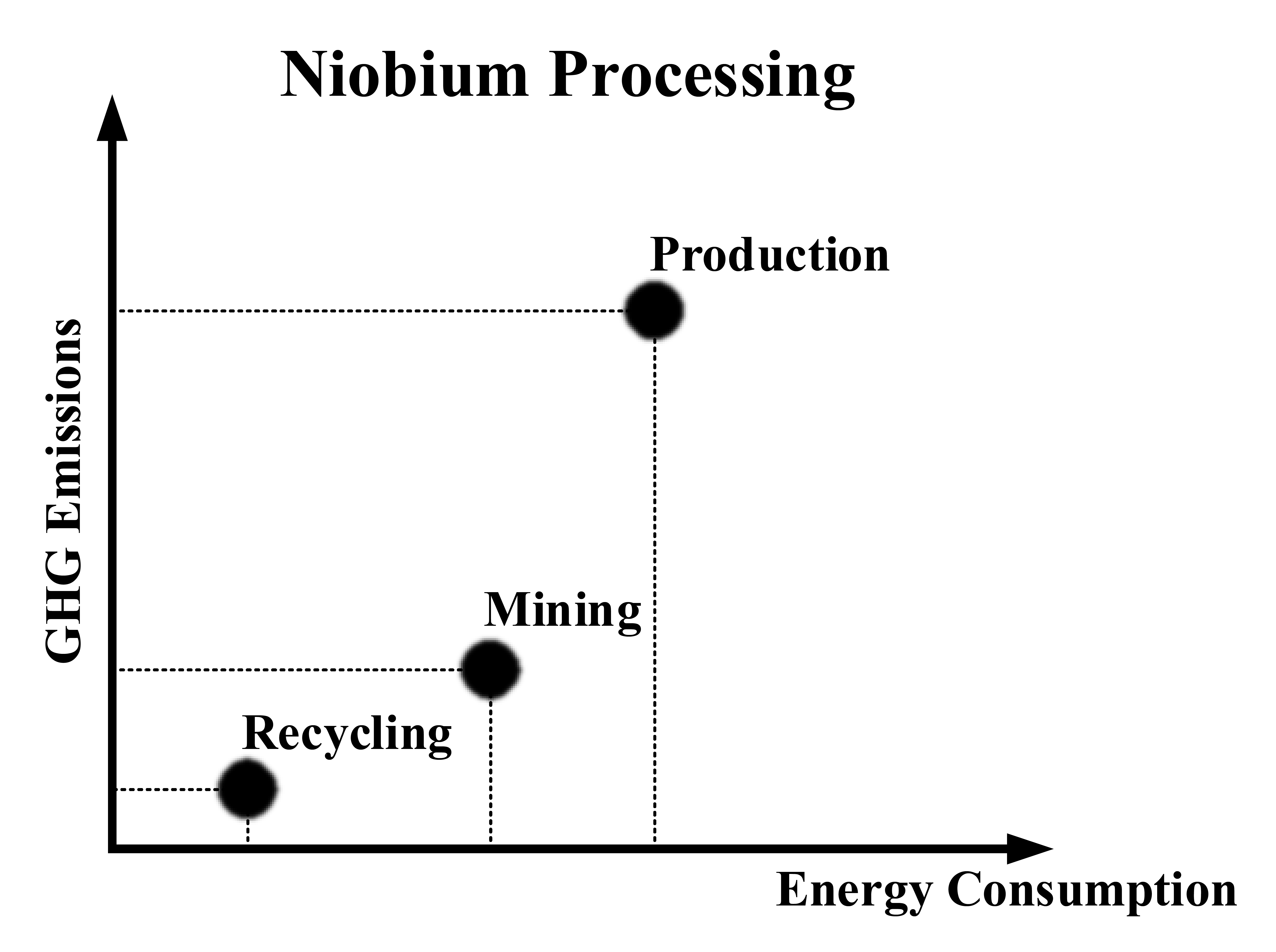
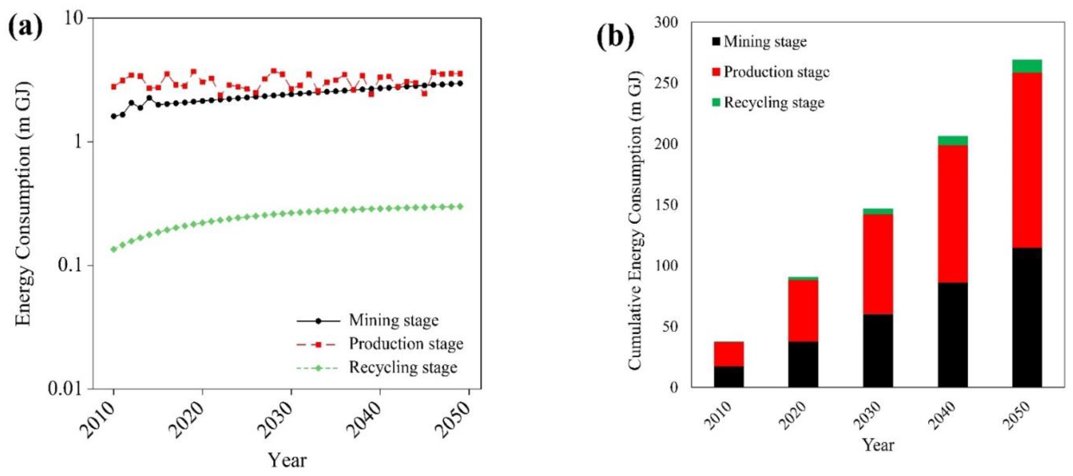
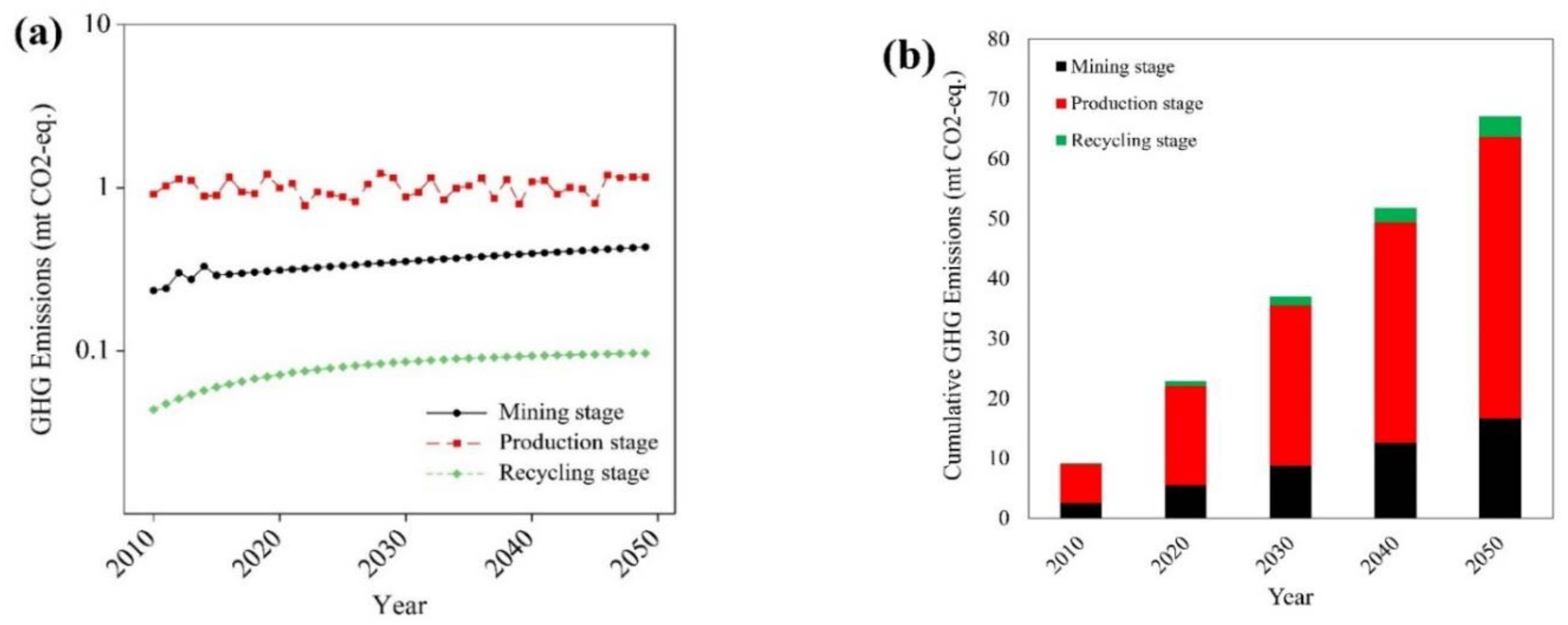
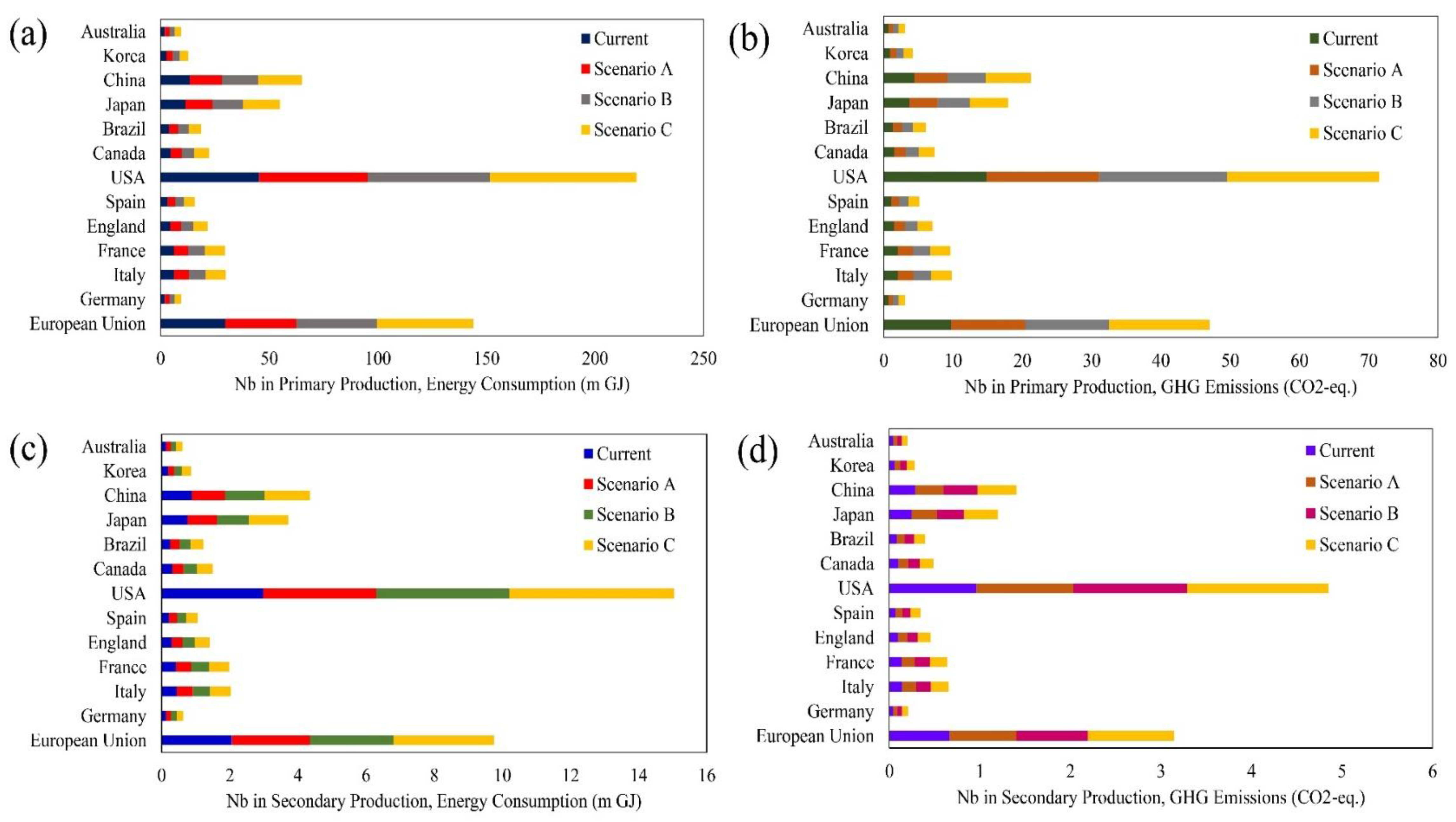
4. Results and Discussion

It is evident that environmental requirements may directly change recycling processes. The balance of energy consumption and GHG emissions from the supply chain helps to determine the environmental sustainability of recycling and the level of investment in recycling. To assess the environmental aspect of niobium recycling, the factors such as energy consumption, GHG emissions, and material flows were quantified and evaluated for all stages of the supply chain. Next, we present the simulation results along with a brief analysis of environmental assessment at different stages of niobium life cycle.

The correlation between energy consumption and GHG emissions is clearly visible in all stages of niobium supply chain. Figure 3a shows that in the mining stage, assuming energy used in hydrofluoric acid dissolution and solvent extraction, the annual mean of energy consumption from the extraction of niobium in years 2010–2050 is around 2.5 million gigajoules (m GJ). Considering six main processes (cold rolling, hot rolling, continuous casting, basic oxygen furnace, blast furnace, sintering/coking) the annual mean of energy used in years 2010–2050 in the production of HSS steels for the automotive industry is around 3 m GJ. In the production stage, energy consumption oscillates due to the dynamics of niobium flow caused by HSS steels demand. Considering energy required in cold rolling, hot rolling, continuous casting, and electric arc furnace processes, in the recycling stage of HSS steels from ELVs, the annual mean level decreases to around 0.3 m GJ of energy. Figure 3b shows that cumulative energy used in years 2010–2050 increases from 17 to 115 m GJ in mining, from 20 to 144 m GJ in production stage and from 0.7 to 11 m GJ, in recycling. It shows that the lowest average energy consumption takes place in recycling stage of niobium supply chain and both production and mining are the most energy consuming processes.

Figure 4 shows total GHG emissions from each stage of niobium lifecycle, focusing on Nb use in HSS steels for the automotive industry. Figure 4a shows that in the mining stage the annual mean of GHG emissions from the extraction of niobium in years 2010–2050 is more than 0.4 million tonnes (mt) CO₂-eq The annual mean of GHG emissions in the production stage of HSS steels for the automotive industry is around 1 mt CO₂-eq in the recycling stage of HSS steels containing niobium from ELVs, the annual mean level decreases to less than 0.08 mt CO₂-eq of emissions. It shows the lowest average GHG emissions for all stages of niobium supply chain. Figure 4b illustrates the increase in cumulative GHG emissions in years 2010–2050. The increase is from 3 to 17 mt CO₂-eq in mining, from 7 to 47 mt CO₂-eq in production stage and from 0.3 to 3 mt CO₂-eq in recycling. As shown in Figure 4a,b, the amount of GHG emitted in production stage is much higher than in the other ones.

In the production and recycling stages, the number of ELVs is a primary variable affecting the energy demand and GHG emissions. The details are shown in

Table 3. Contribution of each country to the increase of energy consumption and GHG emissions in the each stage of the niobium life cycle in the automotive industry (2010–2050).

Country	Production Stage		Recycling Stage
	Energy Consumption (m GJ)	GHG Emission (mt CO2-eq.)	Energy Consumption (m GJ)	GHG Emission (mt CO2-eq.)
European Union (EU-27)	24.2	7.9	1.9	0.6
Germany	1.5	0.5	0.1	0.0
Italy	5.0	1.6	0.4	0.1
France	4.9	1.6	0.4	0.1
England	3.6	1.2	0.3	0.1
Spain	2.6	0.8	0.2	0.1
USA	37.1	12.1	2.8	0.9
Canada	3.7	1.2	0.3	0.1
Brazil	3.1	1.0	0.2	0.1
Japan	9.2	3.0	0.7	0.2
China	10.8	3.5	0.8	0.3
Korea	2.1	0.7	0.2	0.1
Australia	1.5	0.5	0.1	0.0
Global	124.3	40.6	10.0	3.2

. The analysis is limited to the countries with more than 10 million units of automobiles and ELVs in 2010 [14]. The obtained results of simulation show that the highest energy consumption and GHG emissions are accounted for USA, followed by EU, China and Japan, Table 3.

As mentioned in the introduction, previous studies show the growing demand for niobium steel production in the automotive industry. The increase in the share of steel produced from scrap is estimated to be 50–80% until 2050 as shown in several studies [51,52]. In addition, some works also identified the global growth of ELVs numbers and its impact on GHG emissions [12,53]. Due to the previously mentioned significance of a lightweighting strategy by using HSS steel in the automotive industry [11], the likelihood of the growth of niobium demand is quite high [54]. To address this issue, we used a scenario-based approach to identify the impact of the increase of ELVs, and in consequence global demand for niobium, on GHG emissions.

The statistical analysis for predicting the possible growth of numbers of automobiles and ELVs has been presented in other studies [12,50]. They assessed the total car stock from 1950 to 2050 by considering two main variables: Population and car ownership. The results show a possible increase of the number of cars and ELVs by 50–60%. In our work, we assumed the highest value of ELVs growth rate to be 50%. Three scenarios were considered for the growth rate of ELVs to show the changes in cumulative energy consumption and GHG emissions from primary and secondary production of HSS containing niobium in the automotive industry; scenario A, 10%; scenario B, 25%; and scenario C, 50% compared to the baseline scenario (number of ELVs in 2010).

Based on the data available for the reference year (2010), we carried out the analysis assuming the main sources of ELVs are the following countries: Australia, Korea, China, Japan, Brazil, Canada, the USA, Spain, England, France, Italy, Germany and the European Union (EU-27). Figure 5 shows that for the case of 50% increase in the number of ELVs, the estimated GHG emissions from primary production of HSS steels containing niobium will increase by 20% in 2050. While this increase in secondary production would be between 16% and 24% in 2050.

Table 4. Reduction of energy consumption and greenhouse gas emissions, applying Nb in secondary production of HSS steel in the automotive industry (2010–2050).

	Scenario	European Union	Germany	Italy	France	England	Spain	USA	Canada	Brazil	Japan	China	Korea	Australia	Global
Energy Consumption (m GJ)	Current	27.7	1.8	5.8	5.7	4.2	3.0	42.4	4.3	3.6	10.6	12.5	2.5	1.8	133.3
	A	30.4	2.0	6.3	6.2	4.6	3.3	46.5	4.7	4.0	11.6	13.8	2.7	2.0	145.6
	B	34.7	2.2	7.2	7.1	5.2	3.8	52.6	5.4	4.5	13.2	15.6	3.1	2.3	155.6
	C	41.5	2.7	8.7	8.5	6.2	4.5	62.6	6.5	5.4	15.8	18.8	3.7	2.7	161.4
GHG Emissions (mt CO2-eq.)	Current	9.1	0.6	1.9	1.9	1.4	1.0	13.9	1.4	1.2	3.5	4.1	0.8	0.6	43.6
	A	9.9	0.6	2.1	2.0	1.5	1.1	15.2	1.6	1.3	3.8	4.5	0.9	0.6	47.6
	B	11.3	0.7	2.4	2.3	1.7	1.2	17.2	1.8	1.5	4.3	5.1	1.0	0.7	50.9
	C	13.6	0.9	2.8	2.8	2.0	1.5	20.5	2.1	1.8	5.2	6.1	1.2	0.9	52.7

provides the details of the reduction of energy consumption and GHG emissions for each country by using niobium in secondary production of HSS steel in the automotive industry from 2010 to 2050. Globally, around 133–161 m GJ energy could be saved by using Nb in secondary production of HSS steel in the automotive industry. It also contributes to 44–53 mt CO₂-eq, mainly in the USA, followed by the EU, China and Japan.

Figure 6a shows cumulative energy use in mining stage increases from 17 m GJ to 115 m GJ between 2010 and 2050. In production stage, it increases from 20 m GJ to 144 m GJ and in recycling stage, it increases from 0.6 m GJ to 11 m GJ in the same period. These results prove the importance of recycling for saving energy over a long-term period. On average, energy demand in recycling is around 19% of total energy consumption of niobium supply chain. While, production and mining stage requires about 45% and 36%, respectively. The results in Figure 6b show that cumulative global GHG emissions in the mining stage increase from 2.5 mt CO₂-eq in 2010 to 17 mt CO₂-eq in 2050. It is, on average, four times more than GHG emissions in recycling in any scenario. Globally, GHG emissions in the recycling of HSS steel containing niobium will increase from around 0.2–0.3 mt CO₂-eq in 2010 to around 3–5 mt CO₂-eq in 2050 corresponding to 10–50% increase in ELVs number. It shows around 18% reduction of annual emissions between 2010 and 2050 thanks to the reuse of niobium in secondary production rather than primary one. Considering 50% increase in demand, the estimated GHG emissions in the production stage will increase to the highest level of all stages. On average, the production stage accounts for 72% of total emissions followed by mining with 21% and recycling accounted for 7%.

This study presents a holistic view of the supply chain of niobium. The analysis carried out in previous publications had not offered insight into energy consumption and GHG emissions in the different stages of niobium supply chain. Moreover, the previous research has been focused on material flow in mining, production or recycling without showing the dynamics of their mutual relations. It means the previous research considered only one stage of supply chain focusing on supply and demand of material or assessment of various technologies.

The environmental requirements will force countries to introduce new laws and drive the automotive industry towards more sustainable use of resources. In this context, the presented study should be very useful in delivering long-term estimates of environmental performance of niobium supply chain. The results presented in this paper show how niobium recycling can lead to the reduction of annual and cumulative emissions and save energy consumption in a long-term perspective.

5. Limitations of the Study

One of the limitations of this study is a lack of tantalum analysis, which is an important by-product in the niobium value chain. This limitation results from restricting of the presented model to the use of niobium in HSS steel for the automotive industry. Another limitation of this study is the lack of the economic assessment of technologies for primary and secondary production of niobium.

6. Conclusions

This article presents an initial attempt to use dynamic simulation model of niobium supply chain. The dynamic model allows for comprehensive description and analysis of the niobium supply chain in a long-term perspective considering the environmental protection policies related to the reduction of energy consumption and mitigation of emissions. The results show energy demand and GHG emissions in different stages of niobium life cycle—mining, production and recycling.

The results indicate that mining requires 36% of total energy demand and is responsible for 21% of total emissions in niobium supply chain over the period 2010–2050. The production stage consumes around 45% of energy and contributes to 72% of total emissions. The energy used in the recycling constitutes about 19% of total energy demand and generates only 7% of total emission in niobium supply chain. This result highlights the potential benefit of recycling in saving energy and reducing emissions. Globally, the recycling of niobium could save around 133–161 m GJ energy between 2010 and 2050. It also could lead to the reduction of emissions by 44–53 mt CO₂-eq in the same period. The analysis of the results in different countries shows that the highest impact would be observed in the USA, EU, China and Japan. It shows a possibility to reduce annual emissions by 18% in years 2010–2050 thanks to the reuse of niobium in secondary production rather than primary one.

It should be noted that due to the ever-changing dynamics of material flows, further research should update the findings of this study in the near future by considering the newest technologies emerging in every stage of the supply chain.

References

1. Schulz, K.J.; Piatak, N.M.; Papp, J.F. Niobium and Tantalum; US Geological Survey: Reston, VA, USA, 2017.
2. EU Commission, E.-E. Critical Raw Materials for the EU: Report of the Ad-Hoc Working Group on Defining Critical Raw Materials; European Commission: Stadt Brüssel, Belgien, 2010; pp. 1–84. [Google Scholar]
3. Achzet, B.; Reller, A.; Zepf, V.; Rennie, C.; Ashfield, M.; Simmons, J. Materials Critical to the Energy Industry. An Introduction. Available online: https://www.bp.com/content/dam/bp/pdf/sustainability/group-reports/ESC_Materials_handbook_BP_Apr2014.pdf (accessed on 7 January 2019).
4. Nuss, P.; Harper, E.M.; Nassar, N.T.; Reck, B.K.; Graedel, T.E. Criticality of iron and its principal alloying elements. Environ. Sci. Technol. 2014, 48, 4171–4177. [Google Scholar] [CrossRef] [PubMed]
5. Ober, J.A. Mineral Commodity Summaries 2018; US Geological Survey: Reston, VA, USA, 2018.
6. Woydt, M.; Mohrbacher, H. The tribological and mechanical properties of niobium carbides (NbC) bonded with cobalt or Fe3Al. Wear 2014, 321, 1–7. [Google Scholar] [CrossRef] [Green Version]
7. Alves, A.R.; Coutinho, A.D.R. The Evolution of the Niobium Production in Brazil. Mater. Res. 2015, 18, 106–112. [Google Scholar] [CrossRef] [Green Version]
8. Mackay, D.A.R.; Simandl, G.J. Geology, market and supply chain of niobium and tantalum—A review. Miner. Depos. 2014, 49, 1025–1047. [Google Scholar] [CrossRef]
9. Sverdrup, H.U.; Ragnarsdottir, K.V.; Koca, D. An assessment of metal supply sustainability as an input to policy: Security of supply extraction rates, stocks-in-use, recycling, and risk of scarcity. J. Clean. Prod. 2017, 140, 359–372. [Google Scholar] [CrossRef]
10. Steel, S. At the core of the green economy. Future Case Study 2012, 2012, 31. [Google Scholar]
11. Das, S.; Graziano, D.; Upadhyayula, V.K.K.; Masanet, E.; Riddle, M.; Cresko, J. Vehicle lightweighting energy use impacts in US light-duty vehicle fleet. Sustain. Mater. Technol. 2016, 8, 5–13. [Google Scholar]
12. Modaresi, R.; Pauliuk, S.; Løvik, A.N.; Müller, D.B. Global carbon benefits of material substitution in passenger cars until 2050 and the impact on the steel and aluminum industries. Environ. Sci. Technol. 2014, 48, 10776–10784. [Google Scholar] [CrossRef] [PubMed]
13. Widmer, R.; Du, X.; Haag, O.; Restrepo, E.; Wäger, P.A. Scarce metals in conventional passenger vehicles and end-of-life vehicle shredder output. Environ. Sci. Technol. 2015, 49, 4591–4599. [Google Scholar] [CrossRef]
14. Sakai, S.; Yoshida, H.; Hiratsuka, J.; Vandecasteele, C.; Kohlmeyer, R.; Rotter, V.S.; Passarini, F.; Santini, A.; Peeler, M.; Li, J.; et al. An international comparative study of end-of-life vehicle (ELV) recycling systems. J. Mater. Cycles Waste Manag. 2014, 16, 1–20. [Google Scholar] [CrossRef]
15. Jaskula, B.W. Minerals Yearbook; US Geological Survey: Washington, DC, USA, 2013.
16. Patel, Z.; Khul’ka, K. Niobium for steelmaking. Metallurgist 2001, 45, 477–480. [Google Scholar] [CrossRef]
17. Sullivan, J.L.; Burnham, A.; Wang, M. Energy-Consumption and Carbon-Emission Analysis of Vehicle and Component Manufacturing; Argonne National Lab. (ANL): Argonne, IL, USA, 2010. [Google Scholar]
18. Ferreira, B.; Monedero, J.; Marti, J.L.; Aliaga, C.; Hortal, M.; López, A.D. The economic aspects of recycling. In Post-Consumer Waste Recycling and Optimal Production; InTech: London, UK, 2012. [Google Scholar]
19. Cabrera Serrenho, A.; Allwood, J.M. Material stock demographics: Cars in Great Britain. Environ. Sci. Technol. 2016, 50, 3002–3009. [Google Scholar] [CrossRef] [PubMed]
20. Restrepo, E.; Løvik, A.N.; Wäger, P.; Widmer, R.; Lonka, R.; Müller, D.B. Stocks, Flows, and Distribution of Critical Metals in Embedded Electronics in Passenger Vehicles. Environ. Sci. Technol. 2017, 51, 1129–1139. [Google Scholar] [CrossRef] [PubMed]
21. Hutchins, M.J.; Sutherland, J.W. An exploration of measures of social sustainability and their application to supply chain decisions. J. Clean. Prod. 2008, 16, 1688–1698. [Google Scholar] [CrossRef]
22. Brandenburg, M.; Govindan, K.; Sarkis, J.; Seuring, S. Quantitative models for sustainable supply chain management: Developments and directions. Eur. J. Oper. Res. 2014, 233, 299–312. [Google Scholar] [CrossRef]
23. Eskandarpour, M.; Dejax, P.; Miemczyk, J.; Péton, O. Sustainable supply chain network design: An optimization-oriented review. Omega 2015, 54, 11–32. [Google Scholar] [CrossRef] [Green Version]
24. Mirzaei, M.; Bekri, M. Energy consumption and CO2 emissions in Iran, 2025. Environ. Res. 2017, 154, 345–351. [Google Scholar] [CrossRef] [PubMed]
25. Mercure, J.-F.; Pollitt, H.; Bassi, A.M.; Viñuales, J.E.; Edwards, N.R. Modelling complex systems of heterogeneous agents to better design sustainability transitions policy. Glob. Environ. Chang. 2016, 37, 102–115. [Google Scholar] [CrossRef] [Green Version]
26. Azadeh, A.; Arani, H.V. Biodiesel supply chain optimization via a hybrid system dynamics-mathematical programming approach. Renew. Energy 2016, 93, 383–403. [Google Scholar] [CrossRef]
27. Kuipers, K.J.J.; van Oers, L.F.C.M.; Verboon, M.; van der Voet, E. Assessing environmental implications associated with global copper demand and supply scenarios from 2010 to 2050. Glob. Environ. Chang. 2018, 49, 106–115. [Google Scholar] [CrossRef]
28. Forrester, J.W. Industrial dynamics. J. Oper. Res. Soc. 1997, 48, 1037–1041. [Google Scholar] [CrossRef]
29. Choi, C.H.; Cao, J.; Zhao, F. System dynamics modeling of indium material flows under wide deployment of clean energy technologies. Resour. Conserv. Recycl. 2016, 114, 59–71. [Google Scholar] [CrossRef]
30. Sverdrup, H.U.; Ragnarsdottir, K.V. A system dynamics model for platinum group metal supply, market price, depletion of extractable amounts, ore grade, recycling and stocks-in-use. Resour. Conserv. Recycl. 2016, 114, 130–152. [Google Scholar] [CrossRef]
31. Keilhacker, M.L.; Minner, S. Supply chain risk management for critical commodities: A system dynamics model for the case of the rare earth elements. Resour. Conserv. Recycl. 2017, 125, 349–362. [Google Scholar] [CrossRef]
32. Rooney, M.; Nuttall, W.J.; Kazantzis, N. A System Dynamics Study of Uranium and the Nuclear Fuel Cycle. Available online: http://www.econ.cam.ac.uk/research-files/repec/cam/pdf/cwpe1319.pdf (accessed on 7 January 2019).
33. Sverdrup, H.U. Modelling global extraction, supply, price and depletion of the extractable geological resources with the LITHIUM model. Resour. Conserv. Recycl. 2016, 114, 112–129. [Google Scholar] [CrossRef]
34. El Wali, M.; Golruodbary, S.R.; Kraslawski, A. Impact of recycling improvement on the life cycle of phosphorus. Chin. J. Chem. Eng. 2018. [Google Scholar] [CrossRef]
35. Sverdrup, H.U.; Olafsdottir, A.H. A System Dynamics Model Assessment of the Supply of Niobium and Tantalum Using the WORLD6 Model. Biophys. Econ. Resour. Qual. 2018, 3, 5. [Google Scholar] [CrossRef]
36. Sterman, J.D. Business Dynamics: Systems Thinking and Modeling for a Complex World; McGraw-Hill: New York, NY, USA, 2000; Volume 28. [Google Scholar]
37. Schulz, K.; Papp, J. Niobium and Tantalum: Indispensable Twins; US Geological Survey: Reston, VA, USA, 2014.
38. Julião, L.M.Q.C.; Melo, D.R.; Sousa, W.O.; Santos, M.S.; Fernandes, P.C.; Godoy, M.L.D.P. Exposure of workers in a mineral processing industry in Brazil. Radiat. Prot. Dosimetry 2007, 125, 513–515. [Google Scholar] [CrossRef] [PubMed]
39. EU Commission Report on Critical Raw materials for the EU. Retrieved April 2014, 30, 2015.
40. Nikishina, E.E.; Drobot, D.V.; Lebedeva, E.N. Niobium and tantalum: State of the world market, fields of application, and raw sources. Part I. Russ. J. Non-Ferrous Met. 2013, 54, 446–452. [Google Scholar] [CrossRef]
41. Worldwide, D. American Iron and Steel Institute-SMDI Light Vehicle Steel Content. Available online: https://www.autosteel.org/~/media/Files/Autosteel/Research/AHSS/Ducker%20Survey%20Results%20-%20AHSS%20Growth.pdf (accessed on 7 January 2019).
42. Chunbao Charles, X.U.; Cang, D. A brief overview of low CO2 emission technologies for iron and steel making. J. Iron Steel Res. Int. 2010, 17, 1–7. [Google Scholar]
43. Yellishetty, M.; Ranjith, P.G.; Tharumarajah, A. Iron ore and steel production trends and material flows in the world: Is this really sustainable? Resour. Conserv. Recycl. 2010, 54, 1084–1094. [Google Scholar] [CrossRef]
44. Worrell, E.; Reuter, M. Handbook of Recycling: State-Of-The-Art for Practitioners, Analysts, and Scientists; Newnes: Amsterdam, The Netherlands, 2014. [Google Scholar]
45. Ohno, H.; Matsubae, K.; Nakajima, K.; Nakamura, S.; Nagasaka, T. Unintentional Flow of Alloying Elements in Steel during Recycling of End-of-Life Vehicles. J. Ind. Ecol. 2014, 18, 242–253. [Google Scholar] [CrossRef]
46. Balci, O. Verification, validation, and testing. Handb. Simul. 1998, 10, 335–393. [Google Scholar]
47. Golroudbary, S.R.; Zahraee, S.M. System dynamics model for optimizing the recycling and collection of waste material in a closed-loop supply chain. Simul. Model. Pract. Theory 2015, 53, 88–102. [Google Scholar] [CrossRef]
48. Barlas, Y. Formal aspects of model validity and validation in system dynamics. Syst. Dyn. Rev. 1996, 12, 183–210. [Google Scholar] [CrossRef]
49. Kagawa, S.; Nansai, K.; Kondo, Y.; Hubacek, K.; Suh, S.; Minx, J.; Kudoh, Y.; Tasaki, T.; Nakamura, S. Role of motor vehicle lifetime extension in climate change policy. Environ. Sci. Technol. 2011, 45, 1184–1191. [Google Scholar] [CrossRef]
50. Modaresi, R.; Müller, D.B. The role of automobiles for the future of aluminum recycling. Environ. Sci. Technol. 2012, 46, 8587–8594. [Google Scholar] [CrossRef]
51. Pauliuk, S.; Wang, T.; Müller, D.B. Moving toward the circular economy: The role of stocks in the Chinese steel cycle. Environ. Sci. Technol. 2011, 46, 148–154. [Google Scholar] [CrossRef]
52. Björkman, B.; Samuelsson, C. Recycling of steel. In Handbook of Recycling: State-Of-The-Art for Practitioners, Analysts and Scientists; Elsevier: Boston, MA, USA, 2014; pp. 65–83. [Google Scholar]
53. Pauliuk, S.; Dhaniati, N.M.A.; Müller, D.B. Reconciling sectoral abatement strategies with global climate targets: The case of the Chinese passenger vehicle fleet. Environ. Sci. Technol. 2011, 46, 140–147. [Google Scholar] [CrossRef]
54. Moss, R.L.; Tzimas, E.; Kara, H.; Willis, P.; Kooroshy, J. Critical metals in strategic energy technologies. In JRC-Scientific and Strategic RepoStrategic Reports, European Commission Joint Research Centre Institute for Energy and Transport; European Commission: Stadt Brüssel, Belgien, 2011. [Google Scholar]
55. Cullbrand, K.; Magnusson, O. The Use of Potentially Critical Materials in Passenger Cars. Available online: http://publications.lib.chalmers.se/records/fulltext/162842.pdf (accessed on 7 January 2019).
56. Yue, K. Comparative analysis of scrap car recycling management policies. Procedia Environ. Sci. 2012, 16, 44–50. [Google Scholar] [CrossRef]
57. Mueller, D.B.; Cao, J.; Kongar, E.; Altonji, M.; Weiner, P.-H.; Graedel, T.E. Service Lifetimes of Mineral End Uses. Available online: https://minerals.usgs.gov/mrerp/reports/Mueller-06HQGR0174.pdf. (accessed on 7 January 2019).
58. Kim, Y.; Worrell, E. International comparison of CO2 emission trends in the iron and steel industry. Energy Policy 2002, 30, 827–838. [Google Scholar] [CrossRef]
59. Marklund, P.-O.; Nilsson, L.; Rahmn, S.; Jonsson, M.; Svantesson, T.; Hellgren, L.-O. Optimization of a Press Hardened B-pillar by Use of the Response Surface Method; (No. 1999-01-3236). SAE Tech. Paper 1999. [Google Scholar] [CrossRef]
60. Moya, J.A.; Pardo, N. The potential for improvements in energy efficiency and CO2 emissions in the EU27 iron and steel industry under different payback periods. J. Clean. Prod. 2013, 52, 71–83. [Google Scholar] [CrossRef]
61. Ruifrok, R.; Vloemans, R.; Prinsen, S.; Waaijer, A. Best of Both Metals in Body Parts Light Weight Concepts for a Hood; (No. 1999-01-3197). SAE Tech. Paper 1999. [Google Scholar] [CrossRef]
62. van Schaik, M. Advanced High-Strength Steels and Hydroforming Reduce Mass and Improve Dent Resistance of Light Weight Doors In UltraLight Steel Auto Closures Project; (No. 2001-01-3116). SAE Tech. Paper 2001. [Google Scholar] [CrossRef]
63. Yellishetty, M.; Mudd, G.M.; Ranjith, P.G.; Tharumarajah, A. Environmental life-cycle comparisons of steel production and recycling: Sustainability issues, problems and prospects. Environ. Sci. Policy 2011, 14, 650–663. [Google Scholar] [CrossRef]
Figure 1. Conceptual model of niobium global supply chain (application in automotive market).
Recycling 04 00005 g001
Figure 2. Simulation model of niobium global supply chain (application in automotive market).
Recycling 04 00005 g002
Figure 3. Energy consumption levels in different stages of niobium supply chain (2010–2050). (a) Annual energy consumption in different stages. (b) Cumulative energy consumption in different stages.
Recycling 04 00005 g003
Figure 4. Greenhouse gas (GHG) emissions in different stages of niobium supply chain (2010–2050). (a) Annual GHG emissions in different stages. (b) Cumulative GHG emissions in different stages.
Recycling 04 00005 g004
Figure 5. Cumulative energy consumption and greenhouse gas emissions from primary and secondary production of high-strength steel (HSS) containing niobium in automotive markets in the different countries (2010–2050). (a) Energy consumption in production stage. (b) GHG emissions in production stage. (c) Energy consumption in recycling stage. (d) GHG emissions in recycling stage.
Recycling 04 00005 g005
Figure 6. Global energy consumption and greenhouse gas (GHG) emissions in different stages of niobium supply chain (2010–2050). (a) Cumulative energy consumption in different scenarios. (b) Cumulative GHG emissions in different scenarios.
Recycling 04 00005 g006