Environmental Performance Assessment of a Decentralized Network of Recyclable Waste Sorting Facilities: Case Study in Montreal

Abstract

The generation of waste grows yearly. In a centralized approach, more trucks are dispatched to collect the growing demand, with a higher pressure on the road network and greenhouse gas emissions. In contrast, a decentralized approach creates a network of distributed facilities. This study analyzes the impact of a decentralized approach for recyclable waste sorting facilities. It models waste generation, collection, and location of recyclable waste sorting facilities. This approach is applied to a case study in Montreal for polyethylene terephthalate. The case study computes two performance indicators: costs and CO₂ emissions. Six scenarios were developed and compared to a baseline scenario. The results show that decentralization reduces greenhouse gas emissions by 20.3% and operation costs by 8.04%. However, investment costs for the new facilities remain an obstacle. These costs can represent up to 89.7% of the expenses in a decentralized context. Nonetheless, decentralization increases the flexibility of waste collection under growing demand, since the distance to collect one ton has reduced by 35.3% and the average truck load per trip has reduced by 12.8%. To apply the model to the real world, further improvements are required. They span technical, economic, and social acceptability constraints.

1. Introduction

Recycling of waste creates new resources and jobs and diverts waste from landfilling, which helps CO₂ emission reduction [1,2,3,4,5]. In the province of Quebec, the term matières résiduelles (literally translated to residual material), coined in 1997 [6], puts forward the economic potential of waste with recycling and allows us to see waste as a resource. Australia coined a similar term in a circular economy policy [7]. Furthermore, recycling strengthens the closing of material loops, one of the principal circular economy strategies [8], and is a means to attain Sustainable Development Goal 12—sustainable production and consumption [9].

The consideration of waste as a resource is needed, as the amount of waste generated tends to grow. Waste generated on a global scale increased by 54.6% between 2012 and 2016 [10,11] and is expected to double every ten years [12]. In particular, 2.13 Gt of municipal solid waste was generated in 2020, and this is projected to grow to 3.78 Gt by 2050 if no action is taken [13]. Furthermore, American countries tend to generate more waste than European countries. For instance, the average waste generation in the European Union was 534 kg/capita in 2021 [14], while the average landfilled waste in Quebec was 716 kg/capita in the same year [2]. Waste generation growth could, in turn, affect greenhouse gas emissions (GHG) [4,5,15,16,17,18], air quality [18,19,20], soil contamination by landfilling [16,19], and water pollution by leachate generation [16,19,20]. For instance, waste management represented 3.3% of Canada’s GHG emissions in 2022 [21] and 5.2% of the province of Quebec’s in 2021 [22]. For recyclable waste, waste collection has more environmental impacts than recycling, as reported by [18] based on data from the European Commission [23]. Furthermore, recyclable waste management costs varied between 30 USD/t and 80 USD/t in high-income countries, such as Canada in 2016 [11].

Municipalities in the province of Quebec are tasked with municipal waste management [24]. For instance, in Montreal, the city manages waste from residences and small industries, businesses, and institutions such as coffee shops, convenience stores, and small offices [25]. Large industries, businesses, and institutions, such as shopping centres or office towers, manage their own waste [25]. Moreover, three municipal waste streams are collected weekly, with a curbside collection: organic waste, recyclable waste, and household waste [1]. Specifically, recyclable waste is collected by trucks and then sent to a sorting facility. The facility separates the recyclable waste into one of the 42 considered materials, which are regrouped into papers, plastics and fibres, and metals [26]. Rejects are sent to landfills, and the recyclable materials are put into ballots [26]. These ballots are then sold to recycling facilities, which recycle the materials to create new products [2].

Montreal deployed one recyclable waste sorting facility for the city [27] and its population of 1.76 million inhabitants in 2021 [28], while Paris, for instance, had five waste sorting facilities [29] for its 2.13 million inhabitants in 2021 [30]. With the growing demand, this centralized infrastructure can only respond by dispatching more trucks, which increases the pressure on the road network and GHG emissions [4].

Considering the challenges of waste management, one solution is to reduce the distance needed to collect waste, which could reduce GHG. A decentralized approach can help since the recyclable waste sorting facility is nearer to the waste generation source and the population [4,7,31,32]. It could also help the environmental impacts of transportation after waste sorting, as seen in studies about waste transshipment [31,32]. However, decentralization and its potential for application to recycling streams is emergent [33]. To the authors’ knowledge, its impacts in an urban context for municipal recyclable waste remain little studied. In recyclable waste, studies analyze decentralization for electronic waste [33] and electronic vehicle battery dismantling [34]. Other studies focus on its potential for application in different waste streams [4,35,36].

This study aims to detail the performance and limitations of a decentralized recyclable waste sorting facility network in an urban context. From the primary objective, three objectives are derived: (1) elaborate the waste generation behaviour per road, (2) identify the environmental performance associated with the number of recyclable waste sorting facilities inside a municipality, and (3) characterize determining factors in the environmental and economic performance of a decentralized approach.

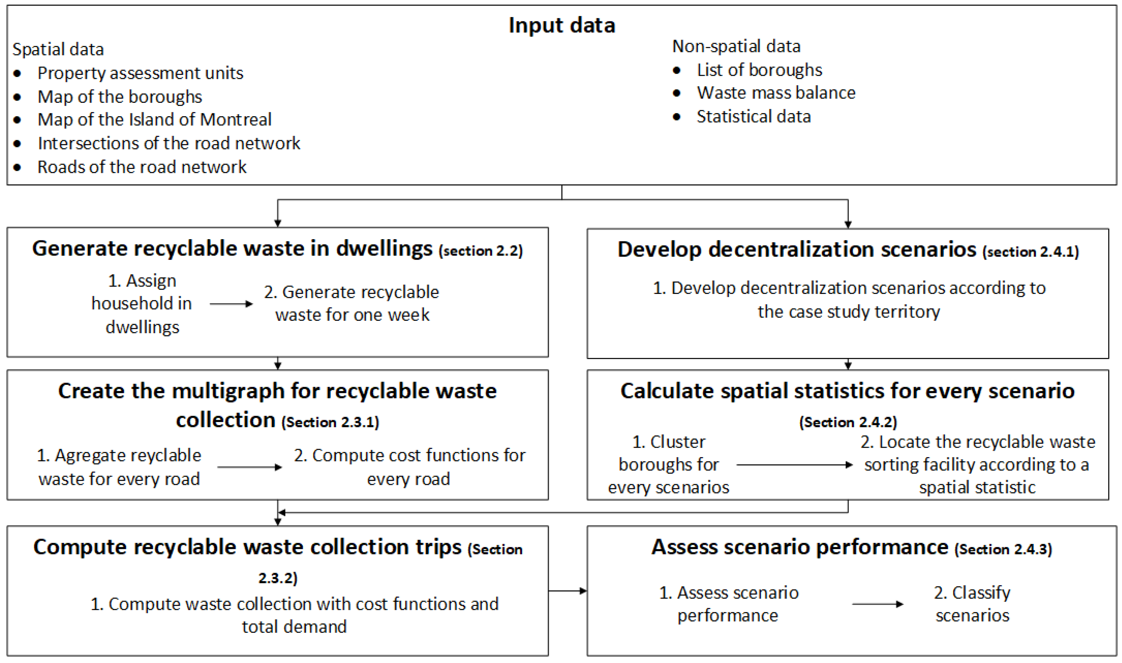
2. Materials and Methods

The methodology consists of a model for recyclable waste generation, recyclable waste collection, and recyclable waste sorting facility decentralization. Figure 1 summarizes the methods used.

Each element of Figure 1 is associated with a section of the current methodology. Scenarios can be constructed simultaneously with recyclable waste generation and the creation of the road network multigraph. However, both the multigraph and the location of recyclable waste sorting facilities are input for the recyclable waste collection trips.

The methodology is implemented in Python 3.8 [37]. NumPy 1.23.4 [38] is used in the recyclable waste generation and collection model. GeoPandas 0.11.1 [39] and SciPy 1.8.1 [40] are used to calculate spatial statistics. Furthermore, some calculations were run before the model in QGIS 3.20.1 [41], such as the map of Montreal boroughs and the conversion of shapefiles into a Geographic JavaScript Object Notation (GEOJSON) format.

2.1. Case Study

The study is applied to the city of Montreal, which comprises 19 boroughs and 15 linked cities [42] and is located on the Island of Montreal. The reference year of this study is 2021. The study considers all the boroughs when planning recyclable waste sorting facilities. However, waste collection is only modelled in seven central boroughs of Montreal. This study excludes linked cities. Figure 2 shows a map of the study area.

Further maps of Montreal will omit the excluded linked cities (in grey in Figure 2). The case study imitates municipal recyclable waste management in Montreal for one week, as described in the introduction. More precisely, it imitates waste collection and waste sorting. This study uses scenarios to assess decentralization. Each scenario’s starting and ending points remain the same for the assessment. The starting point is the generation of recyclable waste in all households. The ending point is the delivery of polyethylene terephthalate (PET). The model excludes shipping other materials since there is only one recycling facility in the territory of the case study, in ANJ [43,44]. PET is assumed to be 1.5% of the municipal recyclable waste generated [25].

Table 1. Initial datasets and input data for the case study.

Dataset	References	Initial Input Data
Boroughs with geographic boundaries	[42,45]	Seven boroughs
Property assessment units	[46]	79,500 property assessment units and 350,000 dwellings
Population statistical data	[28]	645,000 inhabitants and 320,000 households
Waste mass balance	[47]	83.6 kg/capita on average for the seven boroughs
Road network data	[48,49]	28,400 roads totaling 1300 km

shows the initial dataset required for the model and indicates the reference input data from the case study.

2.2. Waste Generation Model

The waste generation model estimates recyclable waste generation by downscaling the municipal recycling waste mass balance to an amount generated per residential building and per week. The municipal waste mass balance combines, in its total, data from residences and small industries, businesses and institutions without distinction [47]. Consequently, the waste generation model assigns all municipal waste to the residences. The property assessment units were filtered to include only residential buildings. The model then stochastically assigns a simulated population to those buildings, assuming that all dwellings are occupied. Algorithm 1 shows the assignation procedure.

Algorithm 1. Household assignment to buildings
Procedure PopulationAssignment ($\mathit{C},\mathit{B}$) For reach $b_i\in B$
	For $k\leftarrow 1 à n_l\left(b\right)$
		${\mathsf{\Sigma }}_l\leftarrow {\sum }_{i=1}^5{C}_{i }$
		$x\leftarrow {\mathcal{U}}_{\mathbb{N}}\{0,{\mathsf{\Sigma }}_i\}$
		$j\leftarrow 1$
		While $x>0$
			$x\leftarrow x-C_{i_r,j}$
			If $x\ge 0$
				$j\leftarrow j+1$
		$p\left(b_i\right)\leftarrow j$
		$C_i\leftarrow C_i-1$

Algorithm 1 relies on a distribution table $C$ computed for each borough with statistical data [28]. Each entry $C_i$ gives the number of households of size $i$ for the given borough. This table is updated during the execution of Algorithm 1 and influences further assignation probabilities of households in buildings. Algorithm 1 draws a random number for the assignment. This number follows the uniform distribution.

Equation (1) gives the generation rate for a building,

$$t_g\left(b\right)={\displaystyle \frac{t_{g_{mr}}\left(a\left(b\right)\right)}{52}}·p\left(b\right),$$

(1)

where:

• $t_g\left(b\right)$: recyclable waste generation rate of one building (kg/week);
• $t_{g_{\mathrm{mr}}}\left(a\left(b\right)\right)$: recyclable waste generation rate for one person in a given borough (kg/capita/year);
• $p\left(b\right)$: number of residents in a building.

The individual recycling waste generation for one person is given in the waste mass balance dataset and is the five-year average between 2014 and 2018 [47]. The generation rate is then used with variation factors, as shown in Equation (2),

$$m_r\left(b\right)=\left(t_g\left(b\right)·0.95+{\mathcal{U}}_{\mathbb{R}}\left[-0.05;0.05\right]·t_g\left(b\right)\right)·c_m,$$

(2)

where:

• $m_r\left(b\right)$: mass of recycling waste for a building for a given week (kg);
• $c_m$: monthly coefficient.

The monthly coefficient $c_m$ is set at 0.97. Its value is taken from a monthly variation in waste generation in which the waste generated in November is closest to the yearly average [50]. Furthermore, the model is validated by comparing the results to the average recycling waste mass balances between 2016 and 2021.

2.3. Waste Collection Model

The modelling of curbside waste collection is based on the capacitated arc routing problem (CARP), since it is best applied for waste collection [51] in high-density territories such as Montreal. The CARP aims to give collection trips that minimize the total time and respect a capacity constraint [15,51]. It requires a multigraph $\mathsf{\Gamma }=(V,E)$, a graph that allows multiple edges to connect the same pair of vertices [52].

The CARP is considered a non-deterministic polynomial-time hard (NP-hard) problem [15,51]. That is, no algorithmic solution can meet the following criteria: (1) the solution is in minimal total time, (2) the algorithm gives a solution in a reasonable time, and (3) the algorithm gives solutions for large amounts of data [53]. In the second criterion, reasonable time refers to a solution of polynomial complexity [53]. Hence, in practice, the first criterion is relaxed to give a satisfactory solution [53,54] given by heuristic solutions, among other approaches. A heuristic is a problem-dependent procedure that generates an acceptable, potentially optimal solution [54].

This section details the waste collection model. It addresses its construction and usage to compute the waste collection trips.

2.3.1. Construction of the Road Network Multigraph

The road network dataset is combined with the waste generation model (Section 2.2) to create a weighted directed multigraph $\mathsf{\Gamma }=(V,E)$. The vertices $V$ are the intersections where the roads meet. The edges $E$ represent the roads. One edge $e\in E$ is created for a unidirectional road. Two edges are created for a bidirectional road, one for each side. Following the multigraph structure of [51], each edge has a demand $w\left(e\right)$ in tons, a collection cost $c_c\left(e\right)$, and a deadheading cost $c_d\left(e\right)$, both in seconds. The demand denotes the waste to be collected at the edge. It aggregates the waste generated for each building on the edge. The collection cost represents the time to collect waste for an edge, while the deadheading cost represents the time to pass through the edge without collecting any waste.

The deadheading cost $c_d\left(e\right)$ is computed with the edge’s speed and the total distance. The speed depends on the type of road. It can be 60 km/h for a highway, 50 km/h for an avenue, and 30 km/h for a local street [17].

Equation (3) presents the collection cost adapted from [55],

$$c_c\left(e\right)=t_s\left(e\right)·n_s\left(e\right)+{\sum }_{b_i\in b\left(e\right)}{t}_w\left(b_i\right)+15,$$

(3)

where:

• $t_s\left(e\right)$: average time between two stops (s);
• $n_s\left(e\right)$: number of stops;
• $b\left(e\right)$: number of buildings on the edge (s);
• $t_w\left(b_i\right)$: walking time from the truck to the building (s).

Equation (3) considers that 15 s is the waiting time at intersections of edges [55]. The number of stops $n_s\left(e\right)$ is estimated by dividing the number of buildings inside the edge by the frequency of stops. A truck typically stops every three buildings on a bidirectional road, and six buildings, three for each side, on a unidirectional one [55]. Equation (4) models the average time between stops, adapted from [55],

$$t_s\left(e\right)={\displaystyle \frac{d_s\left(e\right)}{s_{\max }·\left(1-e^{-k·d_s\left(e\right)}\right)·c}},$$

(4)

where:

• $d_s\left(e\right)$: average distance between stops (m);
• $v_{\max }$: maximum achievable speed by a truck between two stops (km/h);
• $k$: speed coefficient;
• $c$: unit conversion coefficient from km/h to m/s.

The maximum achievable speed $v_{\max }$ is 24.3 km/h, the speed coefficient $k$ is 1.7 × 10⁻² m⁻¹, and the unit conversion $c$ is 0.278 [55]. In Equation (4), a higher value of $k$ suggests a faster acceleration to the maximum achievable speed $v_{\max }$ [55]. The distance between stops $d_s\left(e\right)$ is the average obtained by dividing the distance of the edge by the number of stops. Equation (5) models the walking time $t_w\left(b\right)$, adapted from [55],

$$t_w\left(b\right)=0.86·d_w·⌈{\displaystyle \frac{n_d\left(b\right)}{2}}⌉,$$

(5)

where:

• $d_w$: walking distance (m);
• $n_d\left(b\right)$: number of dwellings inside the building.

The walking distance is fixed at 1.7 m, representing the standard width of a sidewalk in Montreal [56]. Equation (5) assumes one round-trip between the building and the truck for each building. It also assumes that two people collect recyclable waste per truck. It adapts the equation in [55] for the context of an urban area.

The bordering boroughs are integrated into multigraph $\mathsf{\Gamma }=(V,E)$ to ensure graph connectivity and proper model execution. The edges in those surroundings boroughs have a null demand $w\left(e\right)$ and only a deadheading cost $c_d\left(e\right)$.

2.3.2. Algorithmic Application of Waste Collection

The heuristic algorithms described in [51] resolve the CARP with the multigraph modelled in Section 2.3.1. The model uses two heuristics, Extended Path-Scanning and Extended Ulusoy, and chooses the most optimal solution. These heuristics were chosen because they could be applied to a large multigraph without hitting computing limitations. The model also uses the split algorithm described in [51].

Appendix A details how the heuristics were adapted into the current model. More details are presented in [51]. Furthermore, the model integrates the capacity of a truck, established at 9 t. It also extends the heuristics by allowing one to choose the nearest sorting facility at the end of one collection trip.

The implementation is validated on a benchmark dataset given by [57] and compared to the implementation of [51]. The total cost is the only element compared.

2.4. Performance Assessment of Recyclable Waste Sorting Facility Decentralization Scenarios

This section covers the construction of scenarios. It also details the last element of the model, which locates the recyclable waste sorting facilities. Finally, it details the scenarios’ performance assessment.

2.4.1. Decentralization Scenarios

The decentralization scenarios are applied to the 19 boroughs of Montreal. A scenario depicts the number of recyclable waste sorting facilities deployed in Montreal.

Table 2. Division of the territory for each scenario.

Scenario Number	Number of Recyclable Waste Sorting Facilities	Representation of Territory Division
1	1	One recyclable waste sorting facility for Montreal (19 boroughs)
2	2	One recyclable waste sorting facility per ten boroughs
3	4	One recyclable waste sorting facility per five boroughs
4	7	One recyclable waste sorting facility per three boroughs
5	10	One recyclable waste sorting facility per two boroughs
6	19	One recyclable waste facility per borough

presents the scenarios.

The representation of territory division in Table 2 is indicative except for the first and sixth scenarios. A modelling approach (Section 2.4.2) will compute the location of scenarios 2 to 5. A baseline scenario is also considered. This scenario represents the current situation in Montreal, where all recyclable waste is sent to one sorting facility in the territory [27]. Hence, the difference between the first and the baseline is that the modelling approach will compute the first scenario.

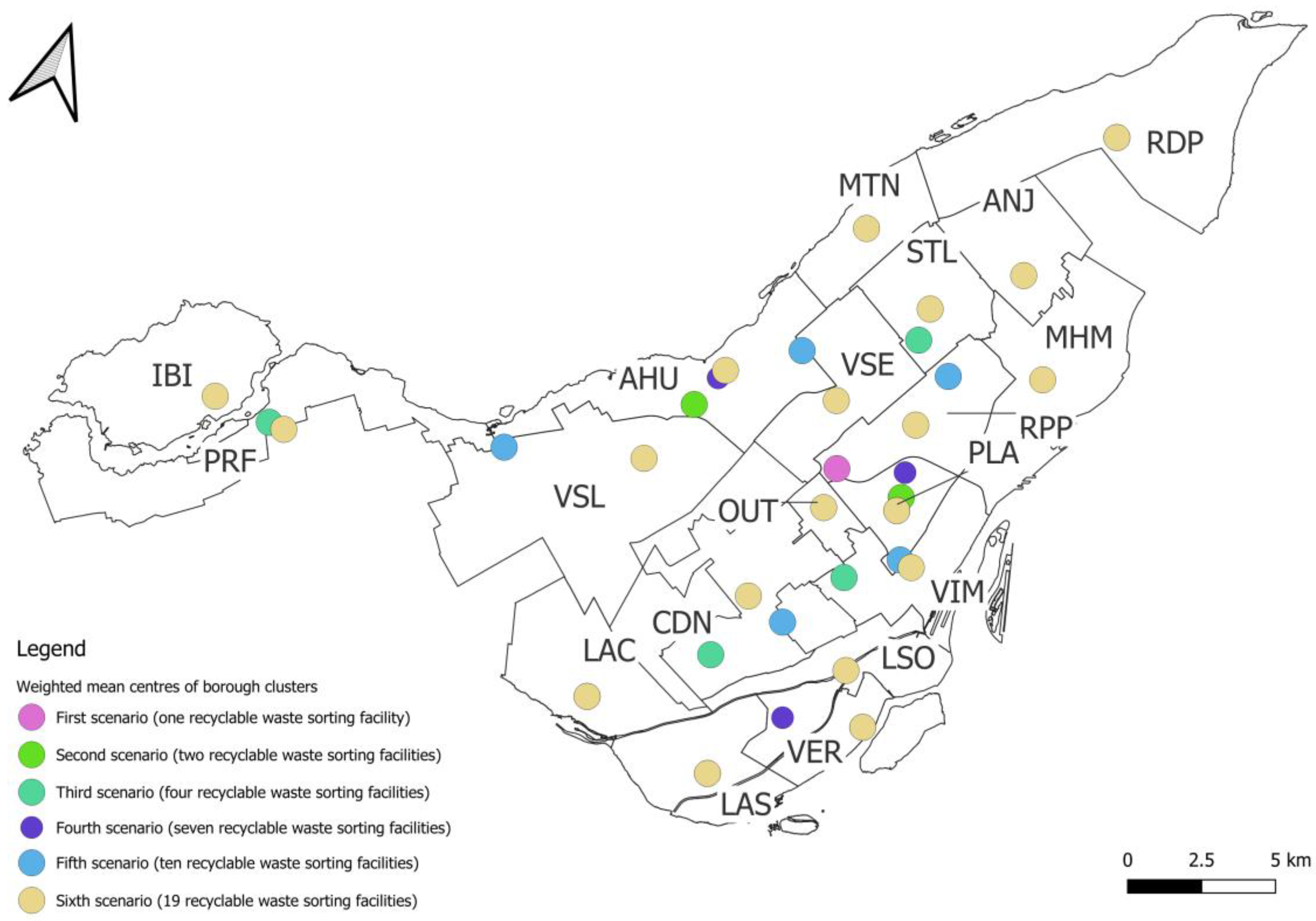
2.4.2. Location of Recyclable Waste Sorting Facilities

Spectral clustering [58,59] and k-means++ [60] cluster boroughs according to the scenario’s number of recyclable waste sorting facilities. This approach is applied from the second to the fifth scenario. For the first scenario, the cluster is the whole city. For the sixth scenario, the cluster is one borough. Like the CARP, optimal clustering is an NP-hard problem [61]. For this problem, the computing approach depends on the input dataset [62]. Hence, spectral clustering was chosen, since it allows a finer representation of the case study with borough and road network data. The k-means++ algorithm was chosen since it is a flexible method that considers the limitations of the k-means algorithm, such as the selection of initial points [60,62].

Spectral clustering is applied to a graph $G=(V,E)$ [58] built from the boroughs and the road network data. In this graph, a vertex is a borough. An edge connects two vertices if the road network can connect them. This rule considers that the road network cannot access certain bordering boroughs [45,49]. Equation (6) gives the Laplacian matrix $L$ of the graph,

$$L=\mathcal{D}-A,$$

(6)

where:

• $\mathcal{D}$: degree matrix of the graph;
• $A$: adjacency matrix of the graph.

The diagonal degree matrix shows the number of edges for a vertex, while the adjacency matrix notes the presence of edges between two vertices [58]. Spectral clustering can be used as a standalone algorithm for two clusters. In this case, the Fiedler eigenvector of the Laplacian matrix gives the clustering [58]. However, when there are more than two clusters, the algorithm must be used with another one. In this case, $k-1$ eigenvectors, associated with the positive and sorted eigenvalues, make the input for k-means++ [60], giving the cluster of boroughs [59]. The model uses the k-means++ implementation available in SciPy [40].

The property assessment unit closest to the weighted mean centre of the cluster becomes the recyclable waste sorting facility. The weighted mean centre is a spatial statistic in which the centre point for a set of points is weighted by a property available in the set of points [63]. It allows the placement of the recyclable waste sorting facility closer to the generation of recyclable waste even if the disaggregated data are unavailable, since waste follows population density [7,64]. For the case study, the centroids of buildings are used as the set of points, and the number of dwellings inside a building is used to weigh the average.

The recycling waste sorting facility has an annual capacity. A small-capacity facility can sort less than 20 kt per year, a medium-capacity facility can sort 20 to 40 kt per year, and a large-capacity facility can sort more than 40 kt per year [65]. The capacity and the corresponding size of the recyclable waste sorting facility are computed by aggregating the recyclable waste to be collected in a year for a cluster. Furthermore, the waste collection model includes the recyclable waste sorting facilities in the boroughs bordering the waste collection.

2.4.3. Scenario Assessment

Scenarios are assessed and compared through one week’s CO₂ emissions and total costs in Canadian dollars. A performance index then aggregates these two indicators.

The costs $c_k$ for a scenario are adapted from [17,66]. The total costs are derived from investment and operating costs [17]. These follow a standard approach observed in the literature [4,17,66,67].

Investment is based on the five-year investment projection of implemented recyclable waste sorting facilities in the province of Quebec, as detailed by [65]. This report constitutes the only investment data available. The annual investment costs depend on the capacity of the recyclable waste sorting facility. They are CAD 2230 K/year for a small-capacity facility, CAD 1930 K/year for a medium-capacity facility, and CAD 2650 K/year for a large-capacity facility [65]. The assessment converts these costs into weekly costs.

The operating costs are the sum of the recyclable waste collection costs and the recyclable waste sorting costs. The recycling waste sorting costs depend on the capacity of the recyclable waste sorting facility. They are CAD 37.55/t for a small-capacity facility, CAD 40.26/t for a medium-capacity, and CAD 40.65/t for a large-capacity [26,65,68]. These costs are modularized since the higher the capacity is, the more residual recyclable waste is rejected and sent to landfilling [65]. They are estimated using the average cost of sorting recyclable waste, which encompasses labour, vehicles, infrastructure, equipment, maintenance, and energy [68] and the average output of the recycling waste sorting facilities [26]. Equation (7) models the collection costs,

$$c_{o_c}={\sum }_{r\in R_c}\left(C_{h_t}·t\left(r\right)+f_d\left(r\right)·{\beta }_{\mathrm{fuel}}\right),$$

(7)

where:

• $C_{h_t}$: hourly cost of trucks (CAD/hour);
• $t\left(r\right)$: time the truck is on the road (h);
• $f_d\left(r\right)$: fuel consumed on the road (L);
• ${\beta }_{\mathrm{fuel}}$: fuel cost (CAD/L).

Diesel is the fuel used by trucks. The hourly rate of trucks is CAD 83/h, and the diesel price is CAD 1.17/L [17]. The hourly cost encompasses various costs in the waste collection process, from the salary of workers to the insurance of the truck [17]. Fuel consumption is based on the Methodology for Calculating Transport Emissions and Energy Consumption (MEET) [69] and reported by [66]. This method was selected since it is an exhaustive method that allows the computation of emissions for a waste collection process [69]. The vehicle category used is a 16–32-ton heavy goods vehicle, found in similar case studies with trucks of nine tons [17,66]. As shown in Equation (8), CO₂, CO, particulate matter (PM), and hydrocarbons (HC) are the pollutants considered. CO₂ is also used for the environmental performance assessment. Equation (8) models fuel consumption $f_d\left(r\right)$,

$$f_d\left(r\right)={\displaystyle \frac{M_{\mathrm{diesel}}·\left(\frac{e_{\mathrm{CO}}\left(r\right)}{M_{\mathrm{CO}}}+\frac{e_{{\mathrm{CO}}_2}\left(r\right)}{M_{{\mathrm{CO}}_2}}+\frac{e_{\mathrm{HC}}\left(r\right)}{M_{\mathrm{HC}}}+\frac{e_{\mathrm{PM}}\left(r\right)}{M_{\mathrm{PM}}}\right)}{{\rho }_{\mathrm{diesel}}}},$$

(8)

where:

• $M_k$: molar mass (g/mol);
• $e_k\left(r\right)$: emission for a road (g);
• ${\rho }_{\mathrm{diesel}}$: density of diesel (kg/L).

Diesel’s density is 0.85 kg/L [70].

Table 3. Molar mass by chemical component. From [69].

Chemical Component	Molar Mass
CO2	28
CO	44
PM	12
HC	14
Diesel	14

presents the molar mass used for fuel consumption.

Equation (9) models the emissions $e_{p_k}$ of a pollutant,

$$e_{p_k}={\sum }_{r\in R_c}\left(e_{p_{k,h}}\left(r\right)\right)+e_{p_{k.c}},$$

(9)

where:

• $R_c$: roads inside a trip (deadheading and collection);
• $e_{p_{k.h}}\left(r\right)$: hot emissions emitted during the trip (g);
• $e_{p_{k,c}}$: cold emissions emitted at the start of a trip (g).

The cold emissions are estimated by multiplying the number of trips and the emission factor for each trip.

Table 4. Cold emission factor by type of pollutant. From [66,69].

Pollutant	Cold Emission Factor
CO2	300
CO	6.00
PM	0.600
HC	2.00

gives the cold emission factor for each pollutant considered.

Hot emissions are computed for each road in the trip. Equation (10) details the hot emissions $e_{p_{k,h}}\left(r\right)$ for a pollutant and a road,

$$e_{p_{k,h}}\left(r\right)={ϵ}_{p,h}\left(r\right)·d\left(r\right),$$

(10)

where:

• ${ϵ}_{p,h}\left(r\right)$: hot emission factor for a pollutant (g/km);
• $d\left(r\right)$: length of the road (km).

Equation (11) models the hot emission factor for a pollutant and a road,

$${ϵ}_{p_{k,h}}\left(r\right)=\left(k_{1_p}+a_p·v\left(r\right)+b_p·{\left(v\left(r\right)\right)}^2+c_p·{\left(v\left(r\right)\right)}^3+{\displaystyle \frac{d_p}{v\left(r\right)}}+{\displaystyle \frac{e_p}{{\left(v\left(r\right)\right)}^2}}+{\displaystyle \frac{f_p}{{\left(v\left(r\right)\right)}^3}}\right)·\left(\left(k_{2_p}+r_p·v\left(r\right)+s_p·{\left(v\left(r\right)\right)}^2+t_p·{\left(v\left(r\right)\right)}^3+{\displaystyle \frac{u_p}{v\left(r\right)}}-1\right)·z\left(r\right)+1\right),$$

(11)

where:

• $k_{1_p}$, $a_p$, $b_p$, $c_p$, $d_p$, $e_p$, $f_p$, $k_{2_p}$, $r_p$, $s_p$, $t_p$, and $u_p$: constants for a pollutant;
• $v\left(r\right)$: speed of the truck on the road (km/h);
• $z\left(r\right)$: relative load of the truck on the road.

The relative load is the ratio of the recyclable waste in the truck divided by the maximum capacity. The MEET gives the constant for the pollutants considered.

Table 5. Constant values for the hot emission factor by type of pollutant. From [66,69].

Pollutant	${\mathit{k}}_1$	$\mathit{a}$	$\mathit{b}$	$\mathit{c}$	$\mathit{d}$	$\mathit{e}$	$\mathit{f}$	${\mathit{k}}_2$	$\mathit{r}$	$\mathit{s}$	$\mathit{t}$	$\mathit{u}$
CO2	765	−7.04	0	6.32 × 10−4	8.83 × 103	0	0	1.27	0	0	0	−0.483
CO	1.53	0	0	0	60.6	117	0	1.17	0	0	0	−0.755
PM	0.184	0	0	1.72 × 10−7	15.2	0	0	1.24	0	0	0	−1.06
HC	0.207	0	0	0	58.3	0	0	1.01	8.89 × 10−4	0	−2.54 × 10−7	0

details those constants.

The MEET was validated at speeds between 10 km/h and 90 km/h [69]. However, experimental data showed that trucks could drive below 10 km/h when collecting recyclable waste. Hence, on those roads, a logarithmic function was resolved on demand with a vertical asymptote when $x=0$ and two points that pass at the values of Equation (10) when the speed is 10 km/h and 90 km/h.

The MEET gives CO₂ emissions and CO₂ used for the environmental assessment through fuel consumption. A performance index $i_s$ compares a scenario to the baseline scenario and measures the costs of avoiding CO₂ emissions, as shown by Equation (12),

$$i_s={\displaystyle \frac{c_s-c_b}{e_b-e_s}},$$

(12)

where:

• $c_s$: costs for the scenario (CAD);
• $c_b$: the costs of the baseline scenario (CAD);
• $e_b$: CO₂ emissions for the baseline scenario (kg);
• $e_s$: CO₂ emissions for the scenario (kg).

The performance index can be interpreted as the costs necessary to avoid CO₂ emissions. It allows for the ranking of different scenarios by grouping the economic and environmental dimensions together. The best scenario is considered the one that has the lowest cost for avoiding CO₂ emissions.

3. Results

This section presents the model’s and the case study’s results. It first details the waste generation and waste collection models.

3.1. Spatialized Recyclable Waste Generation

The assumption that all dwellings are occupied overestimates the population.

Table 6. Dwelling vacancy rate estimates by boroughs.

Boroughs	Vacancy Rate (%)
ANJ	6.84
PLA	11.9
OUT	10.9
RPP	6.16
STL	7.22
VIM	13.6
VSE	6.52
Average for the seven boroughs	9.10

shows an estimated vacancy rate for the boroughs included in the waste collection model. This estimation is based on the number of dwellings available in the property assessment units and the number of households in the statistical dataset.

The overestimation makes comparing the modelled recyclable waste to the mass balances difficult. Hence, the reference datasets are adjusted to follow the same assumptions.

Table 7. Simulated population results per borough.

Boroughs	Reference Population 1	Adjusted Reference Population 2	Simulated Population 3	Error 4 (%)
ANJ	43,200	46,000	46,400	−0.0840
PLA	106,000	120,000	120,000	−0.200
OUT	24,600	27,600	27,500	−0.492
RPP	142,000	151,000	151,000	0.177
STL	79,500	85,700	85,300	−0.501
VIM	105,000	122,000	122,000	0.0908
VSE	145,000	155,000	156,000	0.510
Average for the seven boroughs	645,000	701,000	708,000	0.0461

¹ Value based on [28]; ² value based on a population if all dwellings were occupied; ³ value generated by Algorithm 1; ⁴ error between the adjusted reference population and the simulated population.

presents the reference population, the adjusted reference, and the simulated population.

The error is between −0.501% and 0.510% for each borough. This error is due to the statistical dataset that presents a category of five or more people inside the household [28]. An average household size was estimated for this category, which can cause precision errors. Nonetheless, the error rate remains low even with an over-representation of the population.

Table 8. Simulated recyclable waste generation per borough.

Boroughs	Adjusted Reference of Generated Recyclable Waste (kt/year)	Simulated Generated Recyclable Waste (kt/year)	Error (%)
ANJ	3.11	3.11	0.00343
PLA	11.3	11.3	−0.0750
OUT	2.63	2.62	−0.383
RPP	14.3	14.3	0.284
STL	5.89	5.87	−0.396
VIM	12.7	12.7	0.176
VSE	9.45	9.51	0.612
Average for the seven boroughs	59.4	59.5	0.133

compares the simulation values to an adjusted reference for the recyclable waste generated in one year. The adjusted reference value is obtained using Montreal’s average individual rate between 2014 and 2018 from the waste mass balance [47] and the adjusted population.

The error is between −0.396% and 0.612% for each borough. This error is due to the random factor of 5%, which causes minor disturbances. These disturbances cause the range of errors to be lower than the population. However, the total error rate remains higher than that of the population. Nonetheless, these errors remain low.

3.2. Recyclable Waste Collection Simulation

This section presents modelling results for waste collection based on road network data and road collection trips. Trips are presented for the baseline scenario. The Supplementary Material (Tables S1–S12) presents the trip data for the decentralization scenarios.

3.2.1. Road Network Multigraph

The model generated 16,800 edges for the boroughs included in the waste collection model.

Table 9. Statistics regarding the deadheading cost, collecting cost, and demand for the multigraph.

Statistic	Deadheading Cost (s)	Collection Cost (s)	Demand (kg)
Mean	11.9	84.2	129
Median	8.74	57.9	55.1
Standard deviation	10.7	73.9	228
Minimum	0.440	25.9	0.940
Maximum	209	2010	7680

shows some statistics regarding the properties of the multigraph.

The statistics for the collection costs exclude 7810 edges with a null demand. The sum of collectible recyclable waste in the multigraph is 1.15 kt. The highest collection cost is estimated at 2006 s. The corresponding road has a length of 82 m. This high time is due to there being several residential towers on this street. According to the property assessment dataset, one of these towers is 33 floors tall with 1351 dwellings [46]. This road, among others, is an aberrant value that tends to disperse data. This dispersion can be seen with the mean being higher than the median for all properties. Moreover, the standard deviation for the demand is 1.77 times higher than the mean.

3.2.2. Waste Collection Trips

The baseline scenario computed 137 waste collection trips with a total time of 255 h. This total omits working conditions such as staff and working days.

Table 10. Statistics of the waste collection trips in the baseline scenario.

Statistic	Time (h)	Waste Collected (t)
Mean	1.86	8.42
Median	1.74	8.77
Standard deviation	0.574	0.862
Minimum	0.795	3.64
Maximum	4.10	8.99

presents statistics on the waste collection trips for the baseline scenario. Supplementary Materials present the statistics for each decentralization scenario (Tables S1–S6).

At least half of the trip takes more than 1.74 h, which is higher than the reference method’s one hour [55]. However, the reference method’s suburban context, which is less densely populated, explains this inadequacy. Moreover, each scenario systematically reproduces this inadequacy. Since the performance assessment is based on the difference from the baseline scenario, it remains acceptable for this study.

Trucks tend to be filled, with the median showing that half of the trips collect at least 97.4% of their capacity. The heuristic can explain the minimum of 3.64 t. The last trip built by the heuristic will collect the streets left out during the heuristic’s execution [51], making it harder to reach the maximal capacity.

Table 11. Distance statistics of the waste collection trips in the baseline scenario.

	Absolute Distances (km)			Relative Distances (%)
Statistic	Total	Waste Collection	Deadheading	Waste Collection	Deadheading
Mean	23.1	8.21	14.9	37.0	63.0
Median	21.5	7.05	14.0	37.5	62.5
Standard deviation	9.08	4.91	8.03	17.7	17.7
Minimum	8.59	0.327	3.34	1.91	23.4
Maximum	70.4	25.9	65.8	76.6	98.1

details distances travelled per trip for the baseline scenario. Supplementary Materials present the statistics for each decentralization scenario (Tables S7–S12).

Table 11 shows that most of the trips are deadheading, with 63.0% on average. However, this remains a particular aspect of centralized scenarios. Adding more sorting facilities reduces deadheading, with 45.1% at the highest decentralization level studied (Table S12). This observation confirms that most of the distance is to and from the recyclable waste facilities. Moreover, the minimal collection distance for a trip is about 0.327 km, while the minimal number of roads is 68. Residential towers explain this difference. They have a high quantity of recyclable waste to be collected. In their relative values, the last trip has the maximal deadheading distance and the minimal waste collection distance. It further confirms the behaviour of the heuristics [51]. As the last trip’s goal is to collect all remaining roads, it will mostly carry out deadheading, while the first roads will do the opposite.

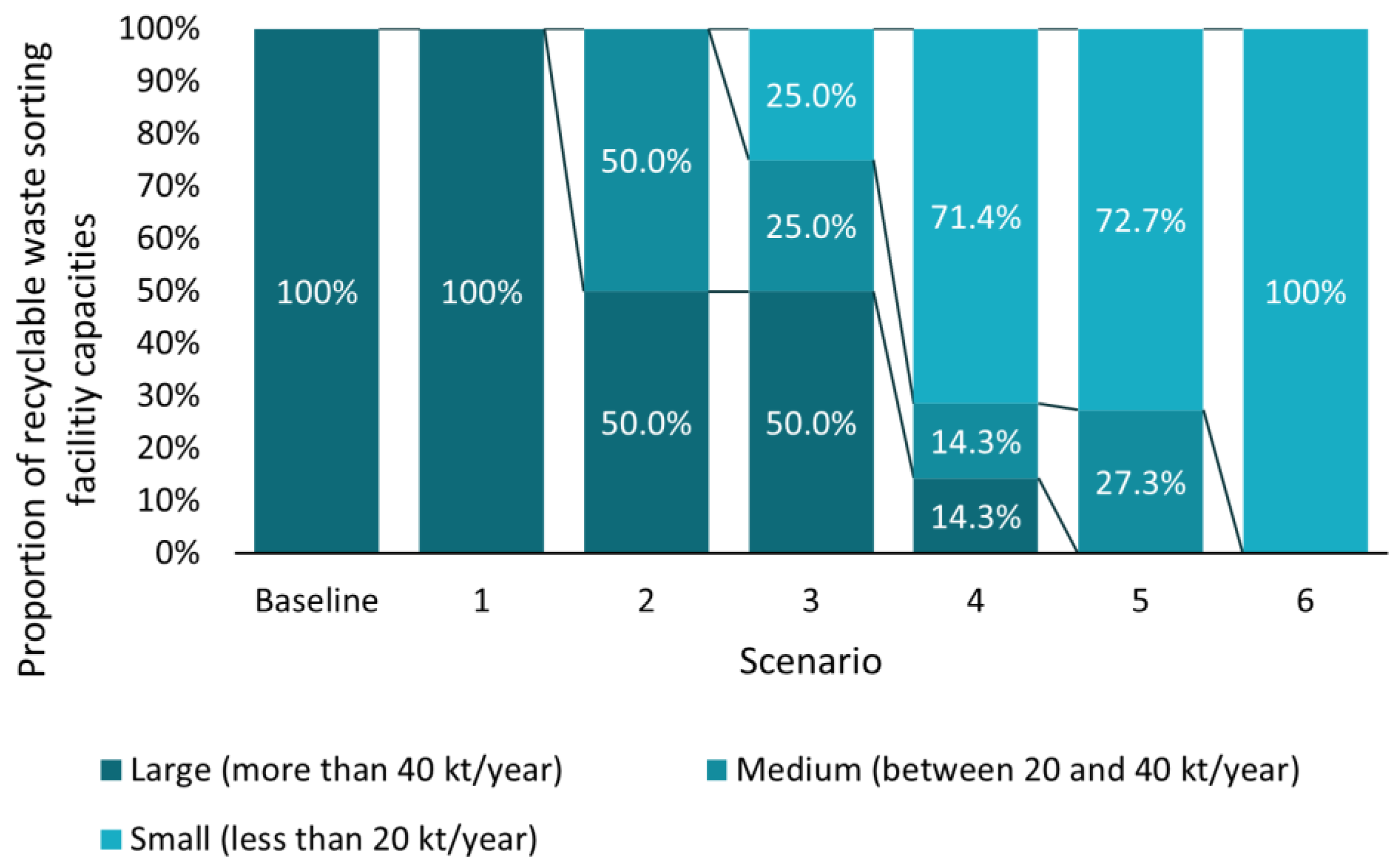
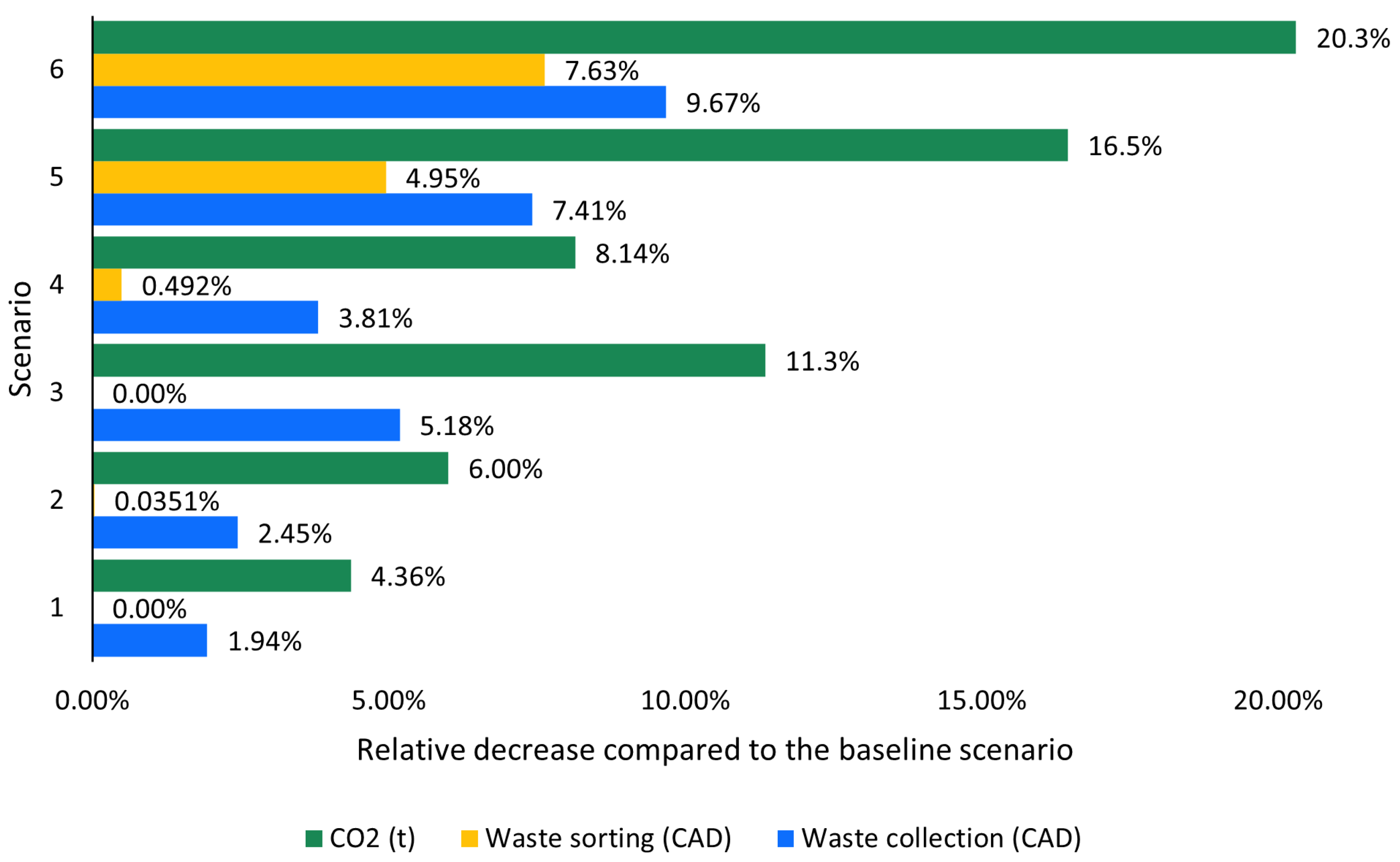
3.3. Decentralization Performance Assessment

This section analyzes the case study’s results. It first details the location of recyclable waste sorting facilities before analyzing the performance of the decentralization scenarios.

3.3.1. Location of Recyclable Waste Sorting Facilities

Spectral clustering and k-means++ were applied to a graph representing Montreal for scenarios 2–5. For scenarios 1 and 6, clusters were manually defined. This graph connects two boroughs if a road network connects them. Figure 3 presents the graph constructed from the methodology. The acronyms are based on the official acronyms [42].

STL, RPP, and VIM are the most connected boroughs (degree five), while IBI is the least connected borough (degree one), followed by RDP, VER, and LAC (degree two). The graph excludes two pairs of bordering boroughs (MTN-ANJ, VSE-OUT) since the road network does not connect them.

Table 12. Borough clusters for recyclable waste sorting facility decentralization.

		Cluster
	Scenario Number	2	3	4	5
	Number of Recyclable Waste Sorting Facilities	2	4	7	10 1
	Cluster Range	A–B	A–D	A–G	A–J
Boroughs	AHU	B	A	A	A
	ANJ	A	A	F	F
	CDN	A	C	F	J
	IBI	B	D	D	F
	LAC	B	B	B	B
	LAS	A	B	E	E
	LSO	A	C	E	J
	MHM	A	A	F	F
	MTN	B	A	A	A
	OUT	A	C	F	H
	PLA	A	C	F	I
	PRF	B	D	A	D
	RDP	A	A	G	G
	RPP	A	A	F	F
	STL	A	A	F	F
	VER	A	B	C	G
	VIM	A	C	F	H
	VSE	B	A	A	A
	VSL	B	B	A	D

¹ Anomalies in clustering results. IBI was clustered in cluster F although it is disconnected from other boroughs.

presents the clusters from the graph. The Supplementary Material presents maps of the clusters (Figures S1–S4).

The clusters in Table 12 should be interpreted per scenario (per column). The anomalies detected in the fifth scenario (ten recyclable waste sorting facilities) were expected since the number of clusters is high. This error constitutes a limitation of the method [58]. Since the location of the waste sorting facility is determined manually, the anomaly is corrected with the assignment of cluster K to IBI in the fifth scenario. Moreover, the number of boroughs within the same cluster varies between each scenario. The most substantial variation is seen in the fourth scenario (seven recyclable waste sorting facilities). In this scenario, the minimum of boroughs per cluster is one, and the maximum is eight.

Both the fourth and fifth scenarios have four single-borough clusters. For the fifth scenario, however, this considers the anomaly in the clustering results. This observation illustrates that spectral clustering, combined with k-means++, favours the isolation of loosely connected boroughs. In the fourth scenario, IBI (degree one), RDP (degree two), VER (degree two), and LAC (degree two) are all in single-borough clusters. Figure 4 shows the weighted mean centre for each cluster and each scenario.

The anomaly in the fifth scenario does not displace the weighted mean centre of its cluster. The recyclable waste sorting facility is in RPP for this scenario and this cluster. The weighted mean centres are gathered in certain boroughs, such as AHU and PLA, which have four distinct weighted mean centres. PLA has five weighted mean centres, one of which is the same for two scenarios (fifth and sixth). In the fifth scenario, VIM’s weighted mean centre is in PLA. The geometry of the borough and the weighted mean centre, which does not forbid the point to go outside its geometry, explains this observation. Another weighted mean centre outside the geometry of the cluster is seen in the B cluster in the third scenario. The recyclable waste sorting facility will still be on a non-residential property nearest the mean centre for those two cases. In the sixth scenario, the residential buildings in PRF and VSL move the weighted mean centre compared to its centroid. A higher population density in one subarea inside the borough explains this movement. In PRF, the polygon is roughly a crescent. Its centroid would be outside the polygon, but the weighted mean centre is inside, at the southern end of the borough. In VSL, the weighted mean centre is more on the eastern side of the borough, in contrast to the centroid. The western side of this borough has mostly industrial buildings [46].

With the weighted mean centre, 33 distinct recyclable waste sorting facilities are deployed in all scenarios. Six of them are deployed in two or three scenarios. The capacity of those facilities varies according to the scenarios, as shown in Figure 5.

Decentralization allows for the progressive reduction of large-capacity recyclable waste sorting facilities and switching towards smaller capacities. Furthermore, like the baseline scenario, the first will deploy a large-capacity recyclable waste sorting facility. Indeed, if only one facility is to be deployed, it must be of a large capacity [4]. Hence, the medium-capacity recyclable waste sorting facilities are deployed in scenarios 2–5, while the small-capacity facilities are deployed in scenarios 3–6.

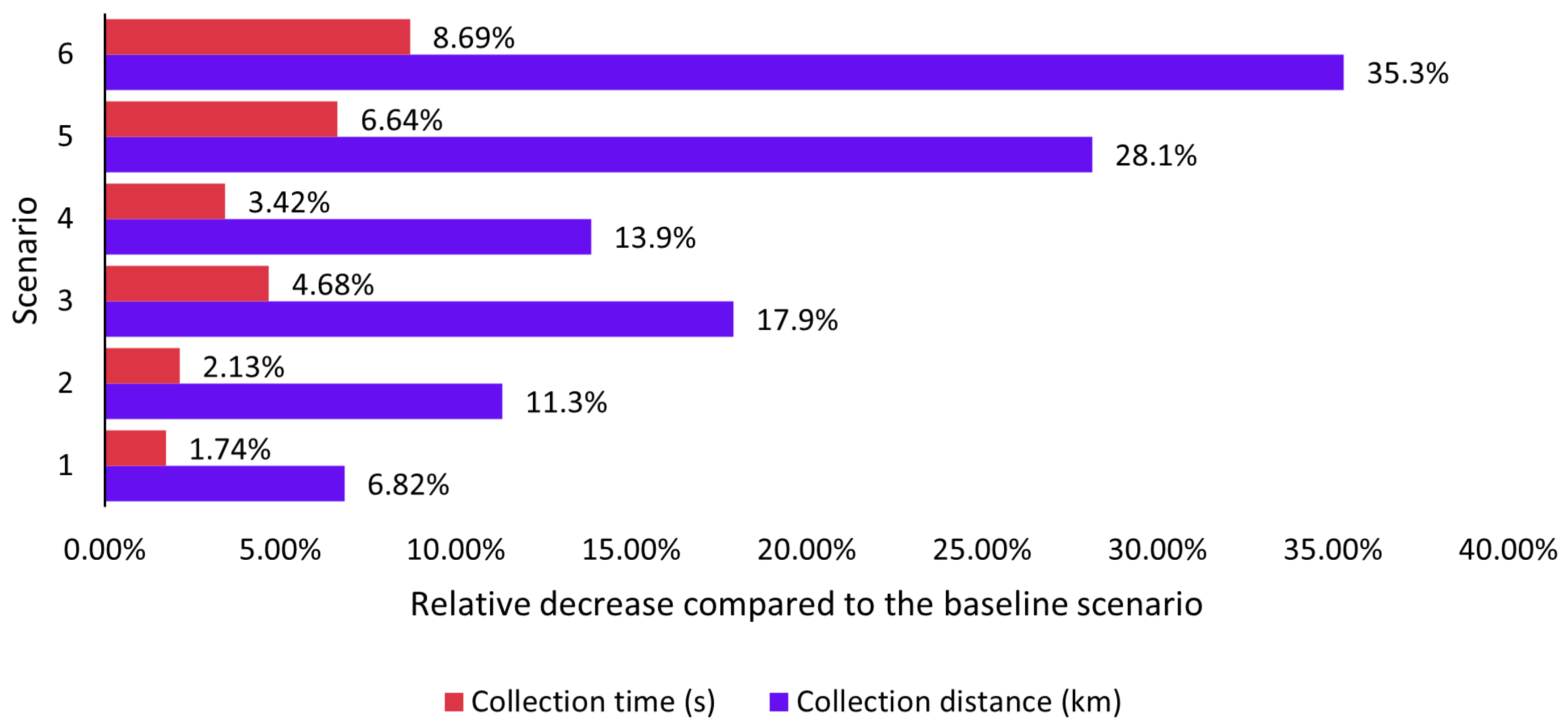
3.3.2. Decentralization Scenario Performance

The performance assessment of scenarios relies on CO₂ emissions and costs. A performance index aggregates these indicators. The decentralization scenarios are compared to the baseline scenarios.

The baseline scenario emits 3.82 t of CO₂ for a week of recyclable waste collection.

Table 13. Emissions of CO₂ and fuel consumption for the baseline scenario.

	Waste Collection		Deadheading		Delivery
Category	Abs.	%	Abs.	%	Abs.	%
CO2 emissions (kg)	2200	57.7	1600	41.9	16.1	0.422
Fuel consumption (L)	845	58.0	607	41.6	6.13	0.420

presents a breakdown of CO₂ emissions and diesel consumption for waste collection, deadheading, and delivery of sorted recyclable waste to a recycling facility. Table S13 in the Supplementary Material presents the emissions data for all the pollutants considered. The Supplementary Material presents the data for each decentralization scenario with all the pollutants considered (Tables S14–S19).

Most of the emissions stem from recyclable waste collection. This observation is explained by a higher fuel consumption when the truck drives slower. For waste collection, a truck drives at an average of 4.96 km/h. In an actual situation, the truck would perform intermittent stops. Delivery has low emissions since there is a small total distance between the recyclable waste sorting facility and the recycling facility, which is 18.5 km in the baseline scenario. In the baseline scenario, the quantity delivered is 17.3 t of PET. Hence, two trucks are sent.

Waste collection has a total distance of 3170 km. The fuel consumption of the baseline scenario is 0.458 L/km, which is in line with other studies [71,72,73]. Furthermore, waste collection emissions remain similar in each decentralization scenario. This similarity is expected since each scenario’s total waste to be collected remains the same. The only possible variation would be in the relative loads of the trucks, which could influence the total emissions. However, these trip changes remain insignificant in the total waste collection emissions. The shorter deadheading introduced by the multiple recyclable waste sorting facilities remains the main driver for reducing emissions in the decentralization scenarios. The delivery of PET, however, is increased with multiple recycling waste sorting facilities, but it has low significance in terms of total emissions.

Four cost categories were studied: recyclable waste collection, recyclable waste sorting, PET delivery, and investment costs. For the baseline scenario, the operating costs are CAD 64.2 K, and the weekly adjusted investment cost is CAD 50.9 K.

Table 14. Baseline scenario costs.

Cost Category	Weekly Cost (K CAD)	Percentage
Investment	50.9	42.2
Waste collection	22.9	19.0
Waste sorting	46.9	38.8
Delivery	0.0363	0.0301
Total	121	100

presents these costs for the studied week and reports an annual cost (weekly cost times 52 weeks). The Supplementary Material presents these costs for each decentralization scenario (Tables S20–S25).

As with pollutants, shorter trips with shorter durations tend to reduce costs. This observation can be seen with delivery costs, representing only 0.0301% of the total cost. It can also be seen in decentralization scenarios, where operating costs are reduced.

In the decentralization scenarios, the performance indicator is the cost of avoiding CO₂ emissions.

Table 15. Performance indexes of each scenario.

Scenario	Emitted CO2 (t)	Total Costs (K CAD)	$\mathbf{Performance} \mathbf{Index} {\mathit{i}}_{\mathit{s}}$ (CAD/kg of Avoided CO2)
Baseline	3.82	120.7	N/A
1	3.82	120.3	−2.59
2	3.65	157.3	160
3	3.59	207.6	201
4	3.51	242.5	392
5	3.19	306.1	295
6	3.04	621.2	646

presents each scenario’s index, CO₂ emissions, and total costs.

The first scenario presents a negative value. This means that costs and emissions are reduced. The scenario configuration explains this result. Since only one recyclable waste sorting facility is deployed in the territory, the investment and recyclable waste sorting costs are the same as the baseline scenario. The recyclable waste sorting facility of the first scenario is nearer to the population and further from the recycling facility. This configuration reduces the waste collection cost by CAD 444 and increases the PET delivery costs by only CAD 12.7, as Table 13 and Table S14 show. It also decreases CO₂ emissions by 166 kg, as Table 14 and Table S20 show. Hence, should the recycling waste sorting facility be replaced, a facility nearer to the population would lower CO₂ emissions and operating costs.

The main driver of total costs is investment costs. These account for most of the costs from the second (56.0%) to the sixth (89.7%) scenarios. They remain the only costs that increase with a higher decentralization of recyclable waste sorting facilities. Without investments, operating costs and CO₂ emissions tend to decrease.

Table 16. Performance indexes of each scenario without investment costs.

Scenario	Operating Costs (K CAD)	$\mathbf{Operating} \mathbf{Performance} \mathbf{Index} {\mathit{i}}_{\mathit{s}}$ (CAD/kg of Avoided CO2)
Baseline	69.79	N/A
1	69.36	−2.59
2	69.26	−2.31
3	68.62	−2.71
4	68.74	−3.38
5	66.26	−5.64
6	64.18	−7.24

presents the performance index without investment costs and operating costs. CO₂ emissions are all emitted from operation activities.

Without investment costs, the performance index is negative for all decentralization scenarios, indicating decreasing costs and emissions. This decrease is higher in the sixth scenario, suggesting the most operational gain with decentralization. These results show that decentralization remains an operational gain. Figure 6 breaks down operating costs and emissions, except for PET delivery as it is negligible.

Waste sorting savings remain on the rise. The fact that smaller-capacity recyclable waste sorting facilities tend to produce less rejected waste [65] explains this observation. The model applies this fact by reducing the costs of sorting recyclable waste. This cost decrease is more accentuated in the fourth scenario, as the smaller-capacity recyclable waste sorting facilities are deployed more frequently in the territory. Waste collection costs and CO₂ emissions rely on distance and time in the waste collection process. Figure 7 shows the relative decrease of those variables.

Deadheading remains the principal driver of changes in collection distance and time, which explains the higher decrease in distances. Time decreases by a lower amount since most of the time is spent on waste collection and not deadheading. However, these reductions are not constant. The fourth scenario does not decrease CO₂ emissions and costs compared to the third scenario. The configuration of the territory explains the result of this scenario. Only one recyclable waste sorting facility is inside the recyclable waste collection territory. The others are in bordering boroughs. As shown in Figure 8, most trips converge on one recyclable waste sorting facility.

In the fourth scenario, 88.6% of the trips end up in the recyclable waste sorting facility in the waste collection territory. With this configuration, the behaviour is closer to a centralized approach. This tendency would be reversed if the study was applied to the city.

4. Discussion

This section interprets the results as a whole. It also reconsiders the scope of the model and its associated limitations, with future research directions to improve it.

4.1. Overview of the Decentralization Approach

The results conclude that a single recyclable waste sorting facility near residential buildings remains a favourable choice due to high investment costs not offset by savings in operation costs. However, certain limits could favour a decentralization approach. Investment, for instance, has a fixed duration. Once the investment is over, all scenarios would see reduced costs and CO₂ emissions.

While results show that investment remains a barrier, infrastructure mutualization can lift it. This approach reduces resource consumption and infrastructure needs [74,75] and involves equipment and space sharing [76]. Waste from another stream (i.e., organic waste) could be included. Including multiple waste streams in decentralization could decrease the total number of facilities to deploy in a territory, but it might increase the capacity of those facilities. The model supports multiple waste streams since the waste generated is an input parameter.

Decentralization changes the configuration of recyclable waste collection trips. A total of 137 trips were necessary in the baseline scenario, while the decentralization scenarios needed between 139 and 157. With more trips, the average time for a trip is between 1.48 h and 1.79 h, compared to 1.86 h in the baseline scenario. The heuristics construct shorter trips, which, in operation, could require more trucks depending on the organization of trips in a working day. The trucks are also, in a decentralized approach, less loaded. On average, the sixth decentralization scenario loads the truck with 7.34 t of recyclable waste compared to 8.42 t in the baseline scenario. Shorter time and distances also reduce the necessary distance to collect one ton of waste. The decentralized scenario has the highest decrease of 35.3%. These results align with the differences in reductions in time and distance. They also align with the literature [4]. Furthermore, a decrease in such distances suggests the higher flexibility of the decentralized approach to changes in recyclable waste generation over time. More waste would need to be generated before the trips are reconfigured. It also suggests reduced pressure on the road network, since fewer heavy trucks are in this network less often, which could help reduce maintenance costs in the infrastructure.

Decentralization sends 1.15 kt of recyclable waste into different facilities, which makes a network configuration of the infrastructure. This configuration allows for redundancy. Should one recycling facility require maintenance, it can stop its operations and send recyclable waste to other facilities. The impact of said maintenance will remain low, since the overall service remains available through other facilities. In a centralized context, the only facility must be kept operational at any moment. Otherwise, waste would have to be sent to another city. However, the distribution of waste remains non-uniform. PET is also distributed, which increases the delivery distances. For instance, in the fourth scenario, one facility sorts 15.7 t of recyclable waste, and two trips are needed between this recyclable waste sorting facility and the recycling facility. Spatial disposition can be a potential barrier to the network configuration. In contrast, facilities can store or dispatch smaller trucks for delivery.

Flexibility to adapt to changes is needed since waste has increased over the years [11,13,25,47]. Implementing a new recyclable waste sorting facility in a decentralized context could also be delayed until needed [4].

Future research could further test these conclusions by changing the population generation rate and examining the results. This generation rate could be changed to examine the impact of waste generation tendencies throughout time and could go further than the year set in the case study. It could also further investigate the impacts on the road network and service disruption. For instance, the impacts of closing one recycling facility in a centralized and decentralized context could be quantified. These investigations would give a more systemic comprehension of decentralization in the urban environment.

4.2. Operationalization of Decentralization Approach

While the study gives insight into the potential of decentralization, further consideration is needed to apply it to a real-world case. In the model, recyclable waste sorting facilities replace non-residential buildings. This approach omits real-world elements, such as the available area for the waste sorting facility and legal or territorial restrictions. These constraints are varied but should be considered [4,67], and could pose an obstacle to implementing the approach [77]. Montreal can leverage waste collection sectors, but will also face challenges regarding lot occupation and social acceptability

On a technical aspect, in Montreal, waste collection sectors denote the day and time when recyclable waste is collected [78]. For instance, some sectors in RPP collect recyclable waste on Tuesday mornings, while other sectors in the same borough are on Monday mornings. The model simplified this reality with a working assumption that waste collection happens on the same day for the city. However, the model must be adjusted to encompass waste collection sectors in this real-world example. The model would require the heuristics to be run multiple times, according to the collection days. Integrating waste collection sectors would primarily impact waste collection trips, since most roads would not have collectible waste for a given day. It could also influence the results of the decentralization approach. Nonetheless, the integration of waste collection sectors could then be used to identify optimal sectors and frequency.

Simulated recyclable waste sorting facilities replace parking lots, schools, industrial buildings, transportation infrastructure buildings, commercial buildings, hospitals, cultural institutions, and places of worship. Only five simulated recyclable waste sorting facilities are implemented on vacant lots. This observation states the importance of considering the actual buildings inside the territory. This consideration, however, can be challenging. Only 10.1% of Montreal’s industrial lots are vacant [79], and this constraint can further limit economic and environmental performance. Hence, as an incremental improvement of the model, it could have a denylist of different building categories and locate recyclable waste sorting facilities in buildings that are not on this list.

The location of recyclable waste sorting facilities can also be a social acceptability challenge. Montreal has faced challenges regarding the social acceptability of implementing an aerobic digester. Public opinion refused the city’s initial propositions in the public consultation stages of the projects via a not-in-my-backyard effect. Indeed, the public opinion stated that the selected boroughs contributed more than their fair share to waste management infrastructure. This forced the city to reconsider the locations [77,80]. Social acceptability indicators, such as population exposure to nuisance [12,81], should therefore be integrated into the model to favour social acceptability.

4.3. Modelling Perspectives

The nature of the study, specifically the comparison of decentralization scenarios to a baseline, allowed working hypotheses to construct the model. One limitation of the model is that some working hypotheses create inaccuracies that hinder analysis of the absolute results of one scenario or application of it to a real-world context. To further gain precision on the model, the methodology of [55] should be applied to a densely populated urban area. The monthly variations should also be applied to the case study territory. The vacancy rate of buildings should be further modelled to pinpoint where they could be. This dataset should be spatialized. The household data should also be reported for the dwelling. For instance, a dataset could report the number of households of a specific size that occupy a particular range of surface area for a dwelling. Moreover, these datasets could distinguish between houses and apartments since houses host larger households that tend to generate more waste [7,82]. The model should consider integrating small industries, businesses, and institutions to achieve a finer interpretation of the results. This change can be made by integrating appropriate property assessment units with an area that is smaller than the living area of the largest residential property assessment unit. It also needs a waste generation model that works for industries, businesses, and institutions. Finally, sensitivities in various input parameters should be considered to gain confidence in an absolute analysis, such as waste generated, waste collection costs and emissions, and recyclable waste sorting costs.

Some system boundaries should also be revisited for modelling improvements. This reconsideration would allow for a more comprehensive analysis when comparing scenarios or analyzing the absolute results of one scenario. Since PET constitutes only 1.5% of municipal recyclable waste, other balloted materials should be considered. This extension would make delivery a more significant contribution to the scenarios’ economic and environmental performance. This extension would require identifying 42 recycling facilities, one for each material, which could be outside of the city studied. The case study’s scope should also be expanded. First, the boundaries could be all the boroughs of Montreal. A second extension could then include all linked cities. These improvements would considerably increase the computations’ size and duration, as doubling the road network’s initial dataset would require eight times more computations [51,53,83]. Hence, the model’s implementation needs an approach that can tackle this increase.

The building and operation of recyclable waste sorting facilities need to be further modelled to strengthen CO₂ emissions and investment costs. For CO₂ emissions, a proper model of the emissions should include the construction of the sorting facility and the necessary investment during the lifetime of the recycling facility. Emissions from the operation of the facility should also be measured. This approach can be based on life cycle analysis as it fits the modelling requirements adequately [84]. If this methodology is selected for CO₂ emissions of the recycling facility, the environmental assessment should consider all GHG emissions, which would be reported as CO₂ equivalents. This model could then give a comprehensive environmental assessment, which could become more significant by deploying more sorting facilities. The model from this study could then study whether the recycling facilities offset the savings made by recyclable waste collection. The model should consider life cycle costs for the investment costs, including the initial construction and the investment during operation. Data can be found for the investment during its operation [65], but the model would have to complete missing data on construction. Having a more comprehensive cost model for recyclable waste would emphasize the offset of high investment costs, which this study has already proved. However, improving the investment costs would allow for the consideration of a break-even analysis and further investigation of the long-term financial sustainability of the decentralization approach.

An extension of the model could implement working conditions. The organization of trips is outside the model’s scope and thus it reports only the total number of trips and the total collection time. However, these trips can be organized on working days to determine the minimum fleet. This extension is possible with a property of NP-Hard problems: switching from one problem to a similar one can be achieved in feasible computing time [53]. Here, heuristics resolve the collection trips. A second algorithm can organize those trips to respect working day lengths.

This study was based on open data from Montreal. However, in its design, the model remains generic, requiring the following spatial datasets, at a minimum: buildings, roads, waste data, and boroughs. Buildings should include the number of dwellings in residential buildings and specify whether a building is residential. Roads should indicate whether the road is a one-way road. Household data allow for a finer waste generation model, but working hypotheses could allow for the omission of this dataset. The minimal datasets require computation and working hypotheses, which the model excluded due to data availability. The road network dataset included the civic numbers on a road, the borough in which the road lies, and a road classification [49]. These properties allowed, respectively, a junction of buildings with civic numbers and road names inside their datasets [46], a filter operation on the borough to reduce computing in the heuristics, and the allocation of different deadheading speeds. If these properties were absent, further computations would have to be made to associate a building with a road and a road with a borough, and a working hypothesis would have to be given for the speed. The hypothesis would be that the speed is constant in the municipality.

5. Conclusions

Waste generation tends to grow over the years [2,10,11,47]. The centralized infrastructure of recyclable waste sorting must respond to the growing demand by dispatching more trucks, leading to an economy of scale, higher pressure on the road network, and GHG emissions [4]. Decentralization is a network approach that could be resilient to failures and reduce operation costs and GHG [4] at the expense of the economy of scale.

This study analyzed the consequences of a decentralization approach to waste collection through a modelling method. The model was applied to a case study in the city of Montreal. In the studied territory, 1.15 kt of recyclable waste was collected on 22,326 roads. Six decentralization scenarios were studied.

Results show that decentralization is primarily an operational advantage. In all scenarios, costs and CO₂ emissions were reduced on an operational basis. The scenario with the most recyclable waste sorting facilities presented a 20.3% decrease in CO₂ emissions and an 8.04% decrease in operation costs. These savings, however, are counteracted by a high investment cost. In the scenario with the highest operation savings, the investment represents 89.7% of the costs. Infrastructure mutualization of multiple waste streams could lift this barrier.

Decentralization allows flexibility in waste collection and recyclable waste sorting. Less recyclable waste is inside the trucks, and less distance is needed to collect one ton of recyclable waste. It could be more resilient to changes or disruptions in recyclable waste generation, which opens the door to different vehicle sizes for waste collection and delivery of sorted recyclable waste. Future research should investigate the integration of multiple waste streams for infrastructure mutualization, the temporal evolution of recyclable waste, and its impacts on a centralized or decentralized approach to further assess the flexibility of decentralization, the integration of facilities in a study territory to lift implementation barriers, and the integration of social acceptability indicators. Finally, the model can be improved by including more modelling for sorting facilities.

References

1. RECYC-QUÉBEC Lexique. Available online: https://www.recyc-quebec.gouv.qc.ca/haut-de-page/lexique (accessed on 28 October 2020).
2. RECYC-QUÉBEC Bilan 2021 de la Gestion des Matières Résiduelles au Québec. 2023. Available online: https://www.recyc-quebec.gouv.qc.ca/actualite/recyc-quebec-diffuse-les-resultats-du-bilan-2021-de-la-gestion-des-matieres-residuelles-au-quebec-bilan-gmr/ (accessed on 27 November 2023).
3. ADEME; Devauze, C.; Koite, A.; Chretien, A.; Monier, V. Bilan National du Recyclage 2010–2019—Évolutions du Recyclage en France de Différents Matériaux: Métaux Ferreux et non Ferreux, Papiers-Cartons, Verre, Plastiques, Inertes du BTP et Bois. 2022. Available online: https://librairie.ademe.fr/dechets-economie-circulaire/5233-bilan-national-du-recyclage-bnr-2010-2019.html#/44-type_de_produit-format_electronique (accessed on 11 March 2022).
4. Kuznetsova, E.; Cardin, M.-A.; Diao, M.; Zhang, S. Integrated Decision-Support Methodology for Combined Centralized-Decentralized Waste-to-Energy Management Systems Design. Renew. Sustain. Energy Rev. 2019, 103, 477–500. [Google Scholar] [CrossRef]
5. Weitz, K.A.; Thorneloe, S.A.; Nishtala, S.R.; Yarkosky, S.; Zannes, M. The Impact of Municipal Solid Waste Management on Greenhouse Gas Emissions in the United States. J. Air Waste Manag. Assoc. 2002, 52, 1000–1011. [Google Scholar] [CrossRef] [PubMed]
6. Bureau D’audiences Publiques sur L’environnement Déchets D’hier, Ressources de Demain; Québec, 1997. Available online: https://www.bape.gouv.qc.ca/fr/dossiers/dechets-hier-ressources-demain/ (accessed on 9 September 2021).
7. Madden, B.; Florin, N.; Mohr, S.; Giurco, D. Spatial Modelling of Municipal Waste Generation: Deriving Property Lot Estimates with Limited Data. Resour. Conserv. Recycl. 2021, 168, 105442. [Google Scholar] [CrossRef]
8. Bocken, N.M.P.; de Pauw, I.; Bakker, C.; van der Grinten, B. Product Design and Business Model Strategies for a Circular Economy. J. Ind. Prod. Eng. 2016, 33, 308–320. [Google Scholar] [CrossRef]
9. United Nations Sustainable Development Sustainable Consumption and Production. Available online: https://www.un.org/sustainabledevelopment/sustainable-consumption-production/ (accessed on 13 March 2025).
10. Hoornweg, D.; Bhada-Tata, P. What a Waste: A Global Review of Solid Waste Management; World Bank: Washington, DC, USA, 2012. [Google Scholar]
11. Kaza, S.; Yao, L.C.; Bhada-Tata, P.; Van Woerden, F. What a Waste 2.0: A Global Snapshot of Solid Waste Management to 2050; World Bank: Washington, DC, USA, 2018; ISBN 978-1-4648-1329-0. [Google Scholar]
12. Ma, Y.; Zhang, W.; Feng, C.; Lev, B.; Li, Z. A Bi-Level Multi-Objective Location-Routing Model for Municipal Waste Management with Obnoxious Effects. Waste Manag. 2021, 135, 109–121. [Google Scholar] [CrossRef]
13. United Nations Environment Programme. Global Waste Management Outlook 2024: Beyond an Age of Waste—Turning Rubbish into a Resource; United Nations Environment Programme: Nairobi, Kenya, 2024. [Google Scholar]
14. Eurostat Municipal Waste Statistics. Available online: https://ec.europa.eu/eurostat/statistics-explained/index.php?title=Municipal_waste_statistics (accessed on 11 March 2025).
15. Duzgun, H.S.; Uskay, S.O.; Aksoy, A. Parallel Hybrid Genetic Algorithm and GIS-Based Optimization for Municipal Solid Waste Collection Routing. J. Comput. Civ. Eng. 2016, 30, 04015037. [Google Scholar] [CrossRef]
16. Lou, X.F.; Nair, J. The Impact of Landfilling and Composting on Greenhouse Gas Emissions—A Review. Bioresour. Technol. 2009, 100, 3792–3798. [Google Scholar] [CrossRef]
17. Tanguy, A.; Villot, J.; Glaus, M.; Laforest, V.; Hausler, R. Service Area Size Assessment for Evaluating the Spatial Scale of Solid Waste Recovery Chains: A Territorial Perspective. Waste Manag. 2017, 64, 386–396. [Google Scholar] [CrossRef]
18. Strange, K. Overview of Waste Management Options: Their Efficacy and Acceptability Page. In Environmental and Health Impact of Solid Waste Management Activities; Royal Society of Chemistry (RSC): London, UK, 2002; pp. 1–51. ISBN 978-0-85404-285-2. [Google Scholar]
19. Ministère des Affaires Municipales et de l’Habitation Rapport Du Ministère Des Affaires Municipales et de L’habitation Présenté à La Commission d’enquête Sur l’état Des Lieux et La Gestion Des Résidus Ultimes. 2021. Available online: https://voute.bape.gouv.qc.ca/dl/?id=00000235537 (accessed on 5 October 2021).
20. Aziz, H.A.; Abu Amr, S.S. Introduction to Solid Waste and Its Management. In Waste Management—Concepts, Methodologies, Tools, and Applications; Information Resources Management Association, Ed.; IGI Global: Hershey, PA, USA, 2020; pp. 1–24. ISBN 978-1-79981-210-4. [Google Scholar]
21. Environment and Climate Change Canada National Inventory Report 1990–2022: Greenhouse Gas Sources and Sinks in Canada. 2024. Available online: https://www.canada.ca/en/environment-climate-change/services/climate-change/greenhouse-gas-emissions/inventory.html (accessed on 12 March 2025).
22. Ministère de l’Environnement, de la Lutte Contre les Changements Climatiques, de la Faune et des Parcs Inventaire Québécois des Émissions de Gaz à Effet de Serre en 2021 et Leur Évolution Depuis 1990. 2023. Available online: https://www.environnement.gouv.qc.ca/changements/ges/2021/inventaire-ges-1990-2021.pdf (accessed on 12 March 2025).
23. Smith, A.; Brown, K.; Ogilvie, S.; Rushton, K.; Bates, J. Waste Management Options and Climate Change. 2011. Available online: https://ec.europa.eu/environment/pdf/waste/studies/climate_change.pdf (accessed on 17 January 2025).
24. Gouvernement du Québec Loi sur la Qualité de L’environnement. 2021. Available online: http://legisquebec.gouv.qc.ca/fr/ShowDoc/cs/Q-2 (accessed on 11 August 2021).
25. RECYC-QUÉBEC Bilan 2018 de la Gestion des Matières Résiduelles au Québec. 2020. Available online: https://www.recyc-quebec.gouv.qc.ca/sites/default/files/documents/bilan-gmr-2018-complet.pdf (accessed on 11 March 2022).
26. Éco Entreprises Québec; RECYC-QUÉBEC Caractérisation des Matières Sortantes des Centres de Tri. 2020. Available online: https://www.recyc-quebec.gouv.qc.ca/sites/default/files/documents/caracterisation-matieres-sortantes-centres-de-tri-2018-2020.pdf (accessed on 28 March 2025).
27. Ville de Montréal Complexe Environnemental de Saint-Michel. Available online: https://montreal.ca/lieux/complexe-environnemental-de-saint-michel (accessed on 21 March 2022).
28. Montréal en Statistiques Annuaire Statistique de l’Agglomération de Montréal—2021. Available online: https://ville.montreal.qc.ca/portal/page?_pageid=6897,68149701&_dad=portal&_schema=PORTAL (accessed on 11 January 2023).
29. Sytcom Centres de Tri. Available online: https://www.syctom-paris.fr/les-installations/centres-de-tri.html (accessed on 11 March 2025).
30. Institut National de la Statistique et des Études Économiques Population Estimates—All—Ville de Paris 2024. Available online: https://www.insee.fr/en/statistiques/serie/001760155 (accessed on 11 March 2025).
31. Höke, M.C.; Yalcinkaya, S. Municipal Solid Waste Transfer Station Planning through Vehicle Routing Problem-Based Scenario Analysis. Waste Manag. Res. 2021, 39, 185–196. [Google Scholar] [CrossRef]
32. Tanguy, A.; Glaus, M.; Laforest, V.; Villot, J.; Hausler, R. A Spatial Analysis of Hierarchical Waste Transport Structures under Growing Demand. Waste Manag. Res. 2016, 34, 1064–1073. [Google Scholar] [CrossRef]
33. Kosai, S.; Kurogi, D.; Kozaki, K.; Yamasue, E. Distributed Recycling System with Microwave-Based Heating for Obsolete Alkaline Batteries. Resour. Environ. Sustain. 2022, 9, 100071. [Google Scholar] [CrossRef]
34. Rallo, H.; Sánchez, A.; Canals, L.; Amante, B. Battery Dismantling Centre in Europe: A Centralized vs Decentralized Analysis. Resour. Conserv. Recycl. Adv. 2022, 15, 200087. [Google Scholar] [CrossRef]
35. Abed Al Ahad, M.; Chalak, A.; Fares, S.; Mardigian, P.; Habib, R.R. Decentralization of Solid Waste Management Services in Rural Lebanon: Barriers and Opportunities. Waste Manag. Res. 2020, 38, 639–648. [Google Scholar] [CrossRef] [PubMed]
36. de Souza, L.C.G.; Drumond, M.A. Decentralized Composting as a Waste Management Tool Connect with the New Global Trends: A Systematic Review. Int. J. Environ. Sci. Technol. 2022, 19, 12679–12700. [Google Scholar] [CrossRef]
37. Python 3.9; Python Software Foundation: Wilmington, DE, USA, 2019; Available online: https://www.python.org/ (accessed on 15 August 2022).
38. Harris, C.R.; Millman, K.J.; van der Walt, S.J.; Gommers, R.; Virtanen, P.; Cournapeau, D.; Wieser, E.; Taylor, J.; Berg, S.; Smith, N.J.; et al. Array Programming with NumPy. Nature 2020, 585, 357–362. [Google Scholar] [CrossRef]
39. Jordahl, K.; den Bossche, J.V.; Fleischmann, M.; McBride, J.; Wasserman, J.; Richards, M.; Badaracco, A.G.; Gerard, J.; Snow, A.D.; Tratner, J.; et al. Geopandas v0.11.1. 2022. Available online: https://zenodo.org/record/6894736 (accessed on 9 September 2022).
40. Virtanen, P.; Gommers, R.; Oliphant, T.E.; Haberland, M.; Reddy, T.; Cournapeau, D.; Burovski, E.; Peterson, P.; Weckesser, W.; Bright, J.; et al. SciPy 1.0: Fundamental Algorithms for Scientific Computing in Python. Nat. Methods 2020, 17, 261–272. [Google Scholar] [CrossRef]
41. QGIS 3.20.1; QGIS Development Team: Laax, Switzerland, 2021; Available online: https://qgis.org (accessed on 16 April 2021).
42. Arrondissement de la Ville de Montréal—Liste. Ville de Montréalé. 2013. Available online: https://donnees.montreal.ca/ville-de-montreal/arros-liste (accessed on 19 February 2021).
43. Lavergne, Inc. Contactez-Nous. Available online: https://lavergne.ca/fr/ (accessed on 20 June 2022).
44. Loubert, A. Évaluation de l’Effet de la Spatialité sur la Performance Environnementale du Recyclage des Bouteilles de PET. Master’s Thesis, École de Technologie Supérieure, Montreal, QC, Canada, 2022. [Google Scholar]
45. Limites Administratives de l’Agglomération de Montréal (Arrondissements et Villes Liées). Ville de Montréal. 2022. Available online: https://donnees.montreal.ca/dataset/limites-administratives-agglomeration (accessed on 21 May 2023).
46. Unités d’Évaluation Foncière. Ville de Montréal. 2017. Available online: https://donnees.montreal.ca/ville-de-montreal/unites-evaluation-fonciere (accessed on 28 October 2020).
47. Matières Résiduelles—Bilan Massique. Ville de Montréal. 2013. Available online: https://donnees.montreal.ca/ville-de-montreal/matieres-residuelles-bilan-massique (accessed on 28 October 2020).
48. Géobase—Nœuds. Ville de Montréal. 2019. Available online: https://donnees.montreal.ca/ville-de-montreal/geobase-noeud (accessed on 12 August 2021).
49. Géobase—Réseau Routier. Ville de Montréal. 2013. Available online: https://donnees.montreal.ca/ville-de-montreal/geobase (accessed on 31 March 2021).
50. Rhyner, C.R. Monthly Variations in Solid Generation. Waste Manag. Res. 1992, 10, 67–71. [Google Scholar] [CrossRef]
51. Lacomme, P.; Prins, C.; Ramdane-Cherif, W. Competitive Memetic Algorithms for Arc Routing Problems. Ann. Oper. Res. 2004, 131, 159–185. [Google Scholar] [CrossRef]
52. Rahman, M.S. (Ed.) Basic Graph Terminologies. In Basic Graph Theory; Undergraduate Topics in Computer Science; Springer International Publishing: Cham, Switzerland, 2017; pp. 11–29. ISBN 978-3-319-49475-3. [Google Scholar]
53. Cormen, T.H. Introduction to Algorithms, 3rd ed.; MIT Press: Cambridge, MA, USA, 2009; ISBN 978-0-262-27083-0. [Google Scholar]
54. Laguna, M.; Martí, R. Heuristics. In Encyclopedia of Operations Research and Management Science; Gass, S.I., Fu, M.C., Eds.; Springer: Boston, MA, USA, 2013; pp. 695–703. ISBN 978-1-4419-1153-7. [Google Scholar]
55. Everett, J.W.; Maratha, S.; Dorairaj, R.; Riley, P. Curbside Collection of Recyclables I: Route Time Estimation Model. Resour. Conserv. Recycl. 1998, 22, 177–192. [Google Scholar] [CrossRef]
56. Ville de Montréal Chartre du Piéton—Document de Consultation; Ville de Montréal, 2006. Available online: https://ville.montreal.qc.ca/portal/page?_pageid=6877,63217598&_dad=portal&_schema=PORTAL (accessed on 26 March 2025).
57. Belenguer, J.M.; Benavent, E. The Capacitated Arc Routing Problem 2003. Available online: https://www.uv.es/belengue/carp.html (accessed on 16 February 2022).
58. Strang, G. 35. Finding Clusters in Graphs. Available online: https://www.youtube.com/watch?v=cxTmmasBiC8 (accessed on 20 July 2022).
59. Liu, J.; Han, J. Spectral Clustering. In Data Clustering; Chapman and Hall/CRC: Boca Raton, FL, USA, 2014; ISBN 978-1-315-37351-5. [Google Scholar]
60. Arthur, D.; Vassilvitskii, S. K-Means++: The Advantages of Careful Seeding. In Proceedings of the Eighteenth Annual ACM-SIAM Symposium on Discrete Algorithms, New Orleans, LA, USA, 7–9 January 2007; Society for Industrial and Applied Mathematics: Philadelphia, PA, USA, 2007; pp. 1027–1035. [Google Scholar]
61. Aloise, D.; Deshpande, A.; Hansen, P.; Popat, P. NP-Hardness of Euclidean Sum-of-Squares Clustering. Mach. Learn. 2009, 75, 245–248. [Google Scholar] [CrossRef]
62. Aggarwal, C.C. An Introduction to Cluster Analysis. In Data Clustering; Chapman and Hall/CRC: Boca Raton, FL, USA, 2014; ISBN 978-1-315-37351-5. [Google Scholar]
63. ESRI Esri Support GIS Dictionary. Available online: https://support.esri.com/en/other-resources/gis-dictionary/term/5d54a903-1839-4687-bb77-92441e72a209 (accessed on 12 August 2022).
64. Cheniti, H.; Cheniti, M.; Brahamia, K. Use of GIS and Moran’s I to Support Residential Solid Waste Recycling in the City of Annaba, Algeria. Environ. Sci. Pollut. Res. 2021, 28, 34027–34041. [Google Scholar] [CrossRef]
65. Langlois-Blouin, S.; Fontaine, C.I.; Boies, M.; Turgeon, N. Diagnostic des Centres de tri du Québec. 2021. Available online: https://www.recyc-quebec.gouv.qc.ca/sites/default/files/documents/rapport-cric-diagnostic-centres-de-tri.pdf (accessed on 11 August 2022).
66. Zsigraiova, Z.; Semiao, V.; Beijoco, F. Operation Costs and Pollutant Emissions Reduction by Definition of New Collection Scheduling and Optimization of MSW Collection Routes Using GIS. The Case Study of Barreiro, Portugal. Waste Manag. 2013, 33, 793–806. [Google Scholar] [CrossRef]
67. Yalcinkaya, S. A Spatial Modeling Approach for Siting, Sizing and Economic Assessment of Centralized Biogas Plants in Organic Waste Management. J. Clean. Prod. 2020, 255, 120040. [Google Scholar] [CrossRef]
68. Éco Entreprises Québec. RECYC-QUÉBEC Allocation des coûts par Activité—Résultats 2016. 2016. Available online: https://www.recyc-quebec.gouv.qc.ca/sites/default/files/documents/allocation-couts-activite-2016.pdf (accessed on 11 August 2022).
69. Transport Research Laboratory; Hickman, J.; Hassel, D.; Joumard, R.; Samaras, Z.; Sorenson, S. Methodology for Calculating Transport Emissions and Energy Consumption. 1999. Available online: https://trimis.ec.europa.eu/sites/default/files/project/documents/meet.pdf (accessed on 4 March 2022).
70. Speight, J.G. 2—Production, Properties and Environmental Impact of Hydrocarbon Fuel Conversion. In Advances in Clean Hydrocarbon Fuel Processing; Khan, M.R., Ed.; Woodhead Publishing Series in Energy; Woodhead Publishing: Sawston, UK, 2011; pp. 54–82. ISBN 978-1-84569-727-3. [Google Scholar]
71. Jaunich, M.K.; Levis, J.W.; DeCarolis, J.F.; Gaston, E.V.; Barlaz, M.A.; Bartelt-Hunt, S.L.; Jones, E.G.; Hauser, L.; Jaikumar, R. Characterization of Municipal Solid Waste Collection Operations. Resour. Conserv. Recycl. 2016, 114, 92–102. [Google Scholar] [CrossRef]
72. Nguyen, T.T.T.; Wilson, B.G. Fuel Consumption Estimation for Kerbside Municipal Solid Waste (MSW) Collection Activities. Waste Manag. Res. 2010, 28, 289–297. [Google Scholar] [CrossRef]
73. Franco González, J.; Gallardo Izquierdo, A.; Commans, F.; Carlos, M. Fuel-Efficient Driving in the Context of Urban Waste-Collection: A Spanish Case Study. J. Clean. Prod. 2021, 289, 125831. [Google Scholar] [CrossRef]
74. Morency, C.; Verreault, H.; Demers, M. Identification of the Minimum Size of the Shared-Car Fleet Required to Satisfy Car-Driving Trips in Montreal. Transportation 2015, 42, 435–447. [Google Scholar] [CrossRef]
75. Sun, S.; Ertz, M. Contribution of Bike-Sharing to Urban Resource Conservation: The Case of Free-Floating Bike-Sharing. J. Clean. Prod. 2021, 280, 124416. [Google Scholar] [CrossRef]
76. Doré, G. De nouveaux lieux d’innovation en France à travers la mutualisation de services. Rev. Organ. Territ. 2021, 30, 141–157. [Google Scholar] [CrossRef]
77. Office de la Consultation Publique de Montréal Centres de Traitement des Matières Organiques. Montréal, 2012. Available online: https://ocpm.qc.ca/fr/consultation-publique/traitement-matieres-organiques (accessed on 27 January 2023).
78. Ville de Montréal Secteurs Info-Collectes 2013. Available online: https://donnees.montreal.ca/ville-de-montreal/info-collectes (accessed on 8 May 2021).
79. Communauté Métropolitaine de Montréal Plan Métropolitain D’aménagement et de Développement. 2012. Available online: https://cmm.qc.ca/planification/plan-metropolitain-damenagement-et-de-developpement-pmad/ (accessed on 8 November 2022).
80. Office de la Consultation Publique de Montréal Centre de Traitement des Matières Organiques—Secteur EST—RDP-PAT. Montréal, 2015. Available online: https://ocpm.qc.ca/fr/consultation-publique/implantation-dun-centre-compostage-dans-secteur-est (accessed on 27 January 2023).
81. Xue, W.; Cao, K. Optimal Routing for Waste Collection: A Case Study in Singapore. Int. J. Geogr. Inf. Sci. 2016, 30, 554–572. [Google Scholar] [CrossRef]
82. Éco Entreprises Québec; RECYC-QUÉBEC Caractérisation des Matières Résiduelles du Secteur Municipal 2015–2018. 2021. Available online: https://www.recyc-quebec.gouv.qc.ca/sites/default/files/documents/caracterisation-secteur-municipal-2015-2018.pdf (accessed on 6 July 2022).
83. Dijkstra, E.W. A Note on Two Problems in Connexion with Graphs. Numer. Math. 1959, 1, 269–271. [Google Scholar] [CrossRef]
84. Jolliet, O.; Saadé, M.; Crettaz, P. Analyse du Cycle de Vie: Comprendre et Réaliser un Écobilan; EPFL Press: Lausanne, Switzerland, 2010; ISBN 978-2-88074-886-9. [Google Scholar]
Figure 1. Overview of the research methodology.
Recycling 10 00058 g001
Figure 2. Case study area. Boroughs’ acronyms are, from left to right, IBI: L’Île-Bizard–Sainte-Geneviève, PRF: Pierrefonds-Roxboro, VSL: Saint-Laurent, LAC: Lachine, AHU: Ahuntsic-Cartierville, LAS: LaSalle, CDN: Côte-des-Neiges–Notre-Dame-de-Grâce, OUT: Outremont, MTN: Montréal-Nord, VSE: Villeray–Saint-Michel–Parc-Extension, VER: Verdun, STL: Saint-Léonard, PLA: Le Plateau-Mont-Royal, LSO: Le Sud-Ouest, RPP: Rosemont–La Petite-Patrie, VIM: Ville-Marie, ANJ: Anjou, MHM: Mercier–Hochelaga-Maisonneuve, and RDP: Rivière-des-Prairies–Pointe-aux-Trembles.
Recycling 10 00058 g002
Figure 3. Graph of connection of Montreal’s boroughs by the road network.
Recycling 10 00058 g003
Figure 4. Weighted mean centres of borough clusters for each scenario. In the fifth scenario, the manual insertion of a waste sorting facility is excluded.
Recycling 10 00058 g004
Figure 5. Proportion of recyclable waste sorting facility capacities by studied scenario.
Recycling 10 00058 g005
Figure 6. Relative decrease in operating costs and CO2 emissions per scenario compared to the baseline scenario.
Recycling 10 00058 g006
Figure 7. Relative decrease in waste collection distance and time per scenario compared to the baseline scenario.
Recycling 10 00058 g007
Figure 8. Truck destination after the last collected road for the fourth scenario.
Recycling 10 00058 g008