Abstract
Capacity decline is the focus of traditional battery health estimation as it is a significant external manifestation of battery aging. However, it is difficult to depict the internal aging information in depth. To achieve the goal of deeper online diagnosis and accurate prediction of battery aging, this paper proposes a data-driven battery aging mechanism analysis and degradation pathway prediction approach. Firstly, a non-destructive aging mechanism analysis method based on the open-circuit voltage model is proposed, where the internal aging modes are quantified through the marine predator algorithm. Secondly, through the design of multi-factor and multi-level orthogonal aging experiments, the dominant aging modes and critical aging factors affecting the battery capacity decay at different life phases are determined using statistical analysis methods. Thirdly, a data-driven multi-factor coupled battery aging mechanism prediction model is developed. Specifically, the Transformer network is designed to establish nonlinear relationships between factors and aging modes, and the regression-based data enhancement is performed to enhance the model generalization capability. To enhance the adaptability to variations in aging conditions, the model outputs are set to the increments of the aging modes. Finally, the experimental results verify that the proposed approach can achieve satisfactory performances under different aging conditions.
1. Introduction
Nowadays, the world is facing increasing fossil energy shortage and environmental pollution problems. New energy electric vehicles and smart grid technologies are gaining more and more attention [1]. Advanced energy storage technology provides a strong impetus for their development. Compared with other energy storage methods, lithium-ion batteries show strong advantages in high energy density, low self-discharge rate, long cycle life, and mobility [2]. However, lithium-ion batteries inevitably suffer performance degradation during use, which in turn affects the safety and reliability of energy storage systems [3]. Therefore, it is essential to monitor the state of health (SOH) of lithium-ion batteries and to predict their future aging pathway [4].
However because the lithium-ion battery is a complex electrochemical system, accurate health prediction is not an easy task [5]. Currently, there are many scholars who have conducted a lot of research in this area. Health prediction methods can be divided into two main categories: model-based methods and data-driven methods. The model-based methods rely on a mathematical model to portray the aging behavior of the battery. A common method is to build a high-precision battery model and then use adaptive algorithms, such as Kalman filters (KFs) [6] and particle filters (PFs) [7], to update the model parameters associated with aging. Equivalent circuit models (ECMs) are widely used due to their simple structure and low computational complexity. In Ref. [8], a particle swarm optimization (PSO) algorithm was developed to estimate both capacity and power fade in a cloud-based battery management system (BMS), where capacity and ohmic resistance in the ECM are used as health indices. In Ref. [9], a health diagnosis method for the battery pack based on an empirical model improved ECM was proposed. A parameter lookup table is established, and virtual measurement of the capacity of the cells and battery pack can be achieved based on partial discharge curves. The ECM-based methods essentially consider the battery model parameters as the SOH. However, the clear physical meaning of these parameters still needs to be discussed [10]. In contrast to the ECMs, the physical meaning of the parameters of the electrochemical model (EM) is well defined. However, the structure of EMs is complex, and the number of model parameters is large, some of which are coupled with each other. The accurate acquisition of parameters remains challenging. In Ref. [11], critical mechanism parameters that dominate electrical performance and capture aging modes were determined through correlation and sensitivity analysis. Then, a non-invasive quantification and health prediction method for aging mechanisms was proposed by combining an EM with the model migration approach. In Ref. [12], an open circuit voltage (OCV) matching model was developed based on a single particle model (SPM) to quantify the aging modes. In addition, the prediction of health and remaining useful life (RUL) was achieved by building semi-empirical models of three aging modes using the PF. There are also some studies that predict aging trajectories by directly building empirical aging models [13]. In Ref. [14], a semi-empirical model based on Coulomb efficiency was developed to capture the battery capacity degradation. In addition, a PF was designed to achieve online updating of model parameters and online health prediction. In Ref. [15], a multi-factor coupled capacity decay model at a low temperature was developed by considering the charging rate, charging temperature, and charging cutoff voltage factors based on the results of orthogonal experiments. This empirical model was successfully applied to the low temperature charging strategy.
With the development of artificial intelligence technology, data-driven methods are becoming increasingly popular [16]. These methods directly predict degradation trends from historical monitoring voltage, current, and temperature data [17]. In Ref. [18], a PSO-nonlinear autoregressive with exogenous input neural network (PSO-NARXNN) approach for health prediction was proposed. Eight features are extracted from partial voltage, capacity, and temperature profiles as network inputs. In Ref. [19], cyclic aging and calendar aging were analyzed under a variety of aging factors. Incremental capacity analysis (ICA) was used to reveal the multi-stage aging mechanism of the battery. Using the incremental capacity data as input, an long short-term memory (LSTM) recurrent neural network (RNN) model was then developed to achieve accurate prediction of capacity decay. This study focused on the effect of multiple external factors on the capacity degradation of lithium-ion batteries. However, the analysis of the essence of capacity decay, the battery aging mechanism, has been neglected. The external manifestations of battery aging are capacity and power degradation. However, the deeper cause is the presence of three aging modes associated with the positive and negative electrodes, namely loss of positive active materials (LAMp), loss of negative active materials (LAMn), and loss of lithium inventory (LLI) [12]. The LAMp and LAMn aging modes are mainly caused by electrode particle cracking, binder decomposition, and loss of electrical contact, etc. These aging modes produce dead lithium at the positive and negative electrodes of the cell that cannot be embedded and disengaged, and increase the cell impedance [20]. The LLI aging mode is mainly due to the growth of SEI film, lithium precipitation, electrolyte decomposition, etc. This aging mode depletes the amount of lithium ions that can migrate during battery charging and discharging, resulting in a decrease in available battery capacity [21]. These three degradation modes provide more in-depth information about the battery health and reveal the mechanism of battery aging. In Ref. [22], a lithium-ion battery degradation diagnosis framework was proposed based on digital twin technology, which allows online monitoring of battery degradation at the electrode level. A multi-step cuckoo search algorithm considering parameter sensitivity differences was developed for aging parameter estimation and aging modes identification. The proposed method could obtain great precision in the presence of sensor noise. In Ref. [23], an offline OCV-based battery aging diagnosis method was proposed. This method fed partial charging curve data directly to a convolutional neural network (CNN), which allowed a fast aging diagnosis at the electrode level.
In summary, there are three possible issues that need to be addressed to achieve the quantification of the aging trajectory of lithium-ion batteries under complex operating conditions. (1) How to achieve a fast and in-depth diagnosis of aging mechanisms based on available measurement signals in the context of big data? (2) What are the dominant aging modes and critical aging factors for battery capacity decay during the whole life cycle? (3) How to achieve online diagnosis and prediction of internal aging mechanisms under complex aging conditions? In order to solve the above problems, a data-driven aging mechanism analysis and degradation pathway prediction method is proposed in this paper. The major contributions are as follows:
- The internal aging mechanism under the external behavior of lithium battery capacity decay is quantified by establishing an OCV reconstruction model. The marine predators algorithm (MPA) is proposed for the identification of the aging mode related parameters;
- The effects of external factors on the internal and external aging behavior of the battery are examined based on orthogonal experiments. The effects of different external factors on capacity decay and internal aging modes at different aging phases throughout the life cycle are quantified by means of the analysis of range (ANOR) and analysis of variance (ANOVA). The dominance of internal aging modes under different operating conditions is investigated using correlation analysis methods;
- A Transformer-based prediction approach is proposed to model the pathway of battery capacity decay and aging modes change under multiple factors. A data enhancement technique based on a multiple regressor integration approach is proposed to empower the model.
The remainder of this paper is outlined as follows: The experimental setup and battery data acquisition are given in Section 2. The battery aging mechanism analysis method is described in Section 3. Section 4 gives the aging factor analysis method. The degradation pathway prediction model is developed in Section 5. Experimental results and evaluation are reported in Section 6. Finally, conclusions are summarized in Section 7.
2. Experiment
In this work, the analysis of the battery aging mechanism and the prediction of the aging path are investigated by taking LiFePO/Graphite batteries as an example. The detailed specifications are listed in Table 1. In order to obtain sufficient supporting data for analysis, it is necessary to conduct a large number of battery experiments. These experiments include: (1) reference performance tests, (2) half battery tests, and (3) multi-factor aging experiments. The reference performance tests are used to obtain the maximum discharge capacity and OCV characteristics of the full cell at the current aging stage. The half battery tests are designed to investigate the open circuit potential (OCP) characteristics of the positive and negative electrodes, and thus the aging mechanism of the cell. The multi-factor aging experiments are dedicated to exploring the effects of different external factors on the aging rate of batteries. For each cell, reference performance tests are performed after hundreds of aging cycles. The half battery tests require destructive disassembly of the battery. After disassembly, the battery cannot be reassembled for the full cell experiments.

Table 1.
Specifications of the batteries.
As the battery ages, the electrode active materials remain stable and the OCP characteristics of the battery electrodes remain almost unchanged [22,24]. However, their quantity and the amount of reacting lithium will change, which has a significant effect on their matching (scaling and translation) [12]. These matching changes lead to variations in the full battery OCV curves and reflect the aging mechanism [11]. In this paper, only a brand new battery is needed for the half battery tests.
2.1. Test Bench
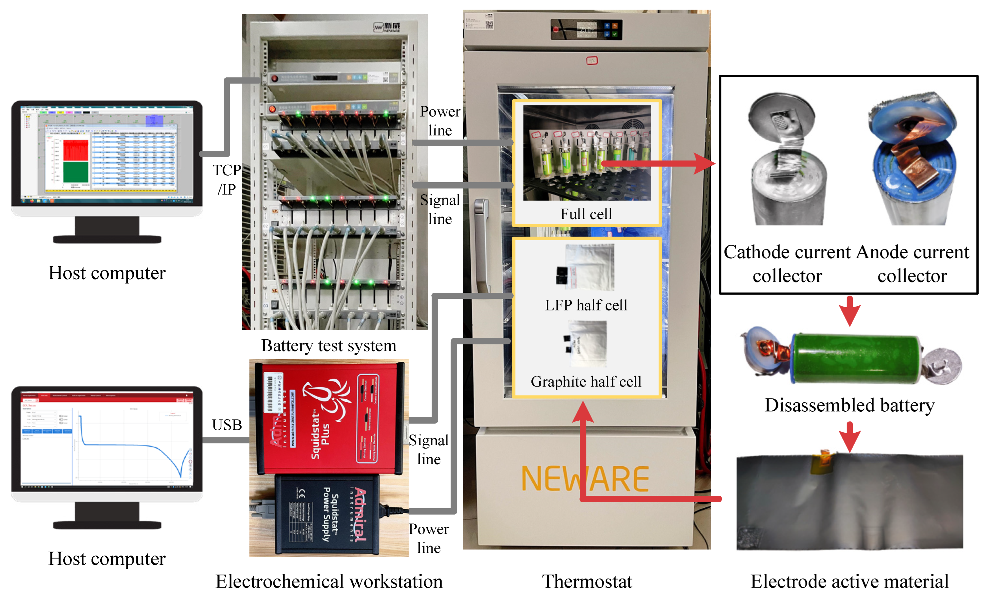
To perform the above experiments, the experimental test bench has been established, as shown in Figure 1, which consists of a battery test system (NEWARE CT-4008T-5V12A), a programmable thermostat (NEWARE MHWX-200), an electrochemical workstation (Admiral Squidstat Plus), test batteries (A123 ANR26650M1B), and host computers. The battery test system is used to program current or power profiles that are loaded onto the test cells to simulate real-world operating conditions with the voltage limit of 0–5 V and a current limit of ±12 A. The thermostat is used to simulate the battery temperature management system and maintain the ambient temperature of the battery. The battery test system uploads the measured experimental data, including current, voltage, power, etc., to the host computer via TCP/IP communication. In addition, in order to investigate the electrode characteristics, the cells were disassembled and made into positive (LFP) and negative (graphite) half cells, respectively. The OCP curves of their positive and negative electrodes are measured using an electrochemical workstation.
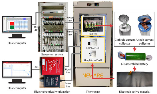
Figure 1.
Experimental setup.
2.2. Reference Performance Tests
The reference performance tests include the capacity test and the OCV test, both of which are conducted at an ambient temperature of 25 °C. The capacity test is performed using constant current and constant voltage (CCCV, 2.5 A/3.6 V/0.125 A) charging and constant current discharging (2.5 A/2.0 V) modes. Repeat charging and discharging at least 3 times until the variation of discharging capacity is less than 3%. The OCV is defined as the terminal voltage of the battery when there is no load, and the battery is in complete equilibrium. The OCV test is to obtain the relationship between OCV and SOC, and to build an OCV-SOC lookup table. Considering the rapid change of OCV at low and high SOC, 13 SOC points are selected: 0, 0.05, 0.1, 0.2, 0.3, 0.4, 0.5, 0.6, 0.7, 0.8, 0.9, 0.98, 1. First, fully charge the battery according to the standard charging mode (CCCV, 2.5 A/3.6 V/0.125 A). The voltage after 2 h of resting is the OCV when the battery SOC is 1. Then, the battery is discharged to the specified SOC point with constant current (2.5 A) and left for 2 h. The voltage at this time is the OCV at the current SOC. Finally, the OCV-SOC curve can be obtained by interpolation. It should be noted that the battery needs to be placed in a 25 °C thermostat for at least 2 h to ensure that the battery temperature is the same as the ambient temperature before conducting the reference performance tests.
2.3. Half Battery Tests
In order to perform half battery tests, it is necessary to make half batteries of the target battery. The preparation process is shown in Figure 1. Drain a brand new battery and disassemble it. Then, use the disassembled positive and negative materials to make half batteries. The reference electrode of the half battery is the lithium electrode. After the half batteries are fabricated, they are placed in a 25 °C thermostat, and OCP tests are performed with an electrochemical workstation. The OCP is defined as the terminal voltage of the half battery when there is no load and the half battery is in complete equilibrium. Before OCP tests, the half batteries are activated through three constant current charge/discharge (10 mA) cycles. The charge and discharge cutoff voltages of the LiFePO half battery are 4.2 V and 2.5 V, respectively. The charge and discharge cutoff voltages of the graphite half battery are 1.2 V and 0.005 V, respectively. Eventually, the approximate OCP curves for the positive and negative electrodes can be obtained by discharging fully charged half batteries with a small current. Some studies have set the discharge current to extremely low rates such as 1/50 C [25] or 1/100 C [26,27]. The extremely small discharge current can greatly reduce the voltage drop across the half-cell impedance, so that the measurement curves can approximate the OCP curves of the electrodes. Further considering the hysteresis effect of LiFePO and the time cost of the experiment, the following OCP test procedures are set up. The LiFePO half battery is discharged at a constant current of 0.5 mA (about 1/120 C rate), and the graphite half battery is discharged at a constant current of 6.7 mA (about 1/60 C rate). It is assumed that, for a particular electrode material, the OCP at a given temperature depends only on the electrode SOC. The results of OCP tests with LiFePO and graphite half-cells are shown in Figure 2. The relationships between OCP and SOC of positive electrode (PE) and negative electrode (NE) are fitted using empirical equations such as Equation (1) [28] and Equation (2) [29]. The parameters are identified through the nonlinear least squares method, as listed in Table 2. The fitting errors of PE OCP are 0.003 V (root mean square error, RMSE) and 1.988% (mean absolute percentage error, MAPE), respectively. The fitting errors of NE OCP are 0.010 V (RMSE) and 0.205% (MAPE), respectively. It can be seen that the fitting results highly overlap with the measured values, indicating that the above empirical equations are reliable and credible:
where and are the OCPs of positive and negative electrodes, respectively. and denote the degrees of lithiation of the positive and negative electrodes (SOC of electrodes), respectively. p, a, b, and are the parameters of the empirical equations.

Figure 2.
The results of OCP tests with LiFePO and graphite half-cells: (a) LiFePO half-cell; (b) graphite half-cell.

Table 2.
The parameters of PE and NE OCP functions.
2.4. Design of Aging Experiments
The aging of batteries is influenced by a variety of external factors. There is a very complex relationship between these external factors and the aging mechanism of the battery. The question is which factors are more important and whether the degree of impact changes as the battery ages. However, it is very costly to perform all possible combinations of experiments in order to understand these relationships and then establish the aging path of the battery under complex stresses. The design of experiments is a technique or procedure that allows the statistical analysis of the obtained experimental results through planned experiments. This technique works by designing a small number of experiments in which several experimental conditions are systematically and systematically changed to obtain sufficient experimental data. Based on these data, mathematical models can be developed to understand the effect of the experimental conditions on the results. Two battery aging experiments are designed in this paper, including: the multi-factor multi-level orthogonal experiments and the one-factor-at-a-time (OFAT) experiments. The orthogonal experiments are used to explore the degree of influence of multiple factors on battery aging and the dominant aging modes during the aging process. The OFAT experiments are used to analyze the effect of each factor on battery aging individually.
2.4.1. Orthogonal Experiments
Orthogonal experiments are based on orthogonal analysis to select a very small but representative set of experiments to study the effects of multiple factors on experimental results simultaneously with much less time and experimental cost. Here, the aging factors considered include: ambient temperature, charge cutoff voltage, charge current, discharge current, and discharge cutoff voltage. It is essential to design reasonable stress levels for all factors. To ensure the safety of the aging test, the stress levels should be within the safe operating range specified in the battery data sheet, as shown in Table 1. In addition, the stress levels should be designed to cover most of the actual battery operating conditions and be as uniformly distributed as possible. Then, three uniform stress levels are designed for each factor, as shown in Table 3. It is assumed that the battery has a good temperature management system and will not be at extremely harsh temperatures, so three temperature levels are set: 25 °C, 45 °C, and 5 °C. The charging current uses the standard and fast charging currents recommended in the datasheet as the upper and lower limits, and then three stress levels were set uniformly: 10 A, 6.25 A, and 2.5 A. The battery can be continuously discharged up to 50 A. However, if discharged continuously with 50 A current, the battery will be empty in 3 min, which is not quite in line with the actual use. Here, the stress level of the discharge current is set to the same as the charge current. In addition, to investigate the effect of different voltage operation intervals on battery aging, three different levels of charge cutoff voltage (3.6 V, 3.5 V and 3.4 V) and discharge cutoff voltage (2 V, 2.5 V and 3 V) are set respectively. Therefore, a five-factor three-level orthogonal experiment is designed. However, there is no standard orthogonal table with exact correspondence. Then, the alternative nearly orthogonal design [30] is constructed using the public allpairs tool. The orthogonal experimental scheme is formulated as shown in Table 4.

Table 3.
Aging factors and levels.

Table 4.
Orthogonal experimental scheme.
2.4.2. OFAT Experiments
The OFAT experimental scheme is formulated as shown in Table 5. Cell 1 is considered the reference cell. The effects of changes in each factor on battery aging are then analyzed separately by varying the level of just one of the five influencing factors. The battery current is usually dynamic during the actual use. Here, the discharge current profile of cell 19 is set to the Highway Fuel Economy Test (HWFET) operating condition. For comparison, the average current of HWFET operation is set to 2.5 A. In addition, cell 18, which varies the level of two factors ( and ) in the cell aging condition, is added for subsequent validation of the generalizability of the aging model.

Table 5.
OFAT experimental scheme.
3. Battery Aging Mechanism Analysis
The external manifestations of battery aging are capacity and power degradation. However, the deeper reason lies in the existence of three aging modes associated with the positive and negative electrodes of the battery, namely LAMp, LAMn, and LLI. A nondestructive aging mode analysis method is proposed, and the full life-cycle aging mode is quantified using a global optimization method.
3.1. Aging Mode Analysis
The OCV of the full cell () is defined as the difference between the OCP of the positive and negative electrodes, which can be calculated as follows:
where the electrodes SOC () can be calculated as follows:
where I denotes the load current, which is positive when the cell discharges. and are the maximum capacities of the positive and negative electrode active materials, respectively.
The above calculation method is very similar to the definition of SOC for a full cell as shown below:
where s and Q are the SOC and maximum available capacity of the full cell. Hence, and can also be considered as the PE SOC and NE SOC. Then, the relationship between electrode SOC and full cell SOC can be established as follows:
where denotes the electrode SOC when the cell SOC is zero.
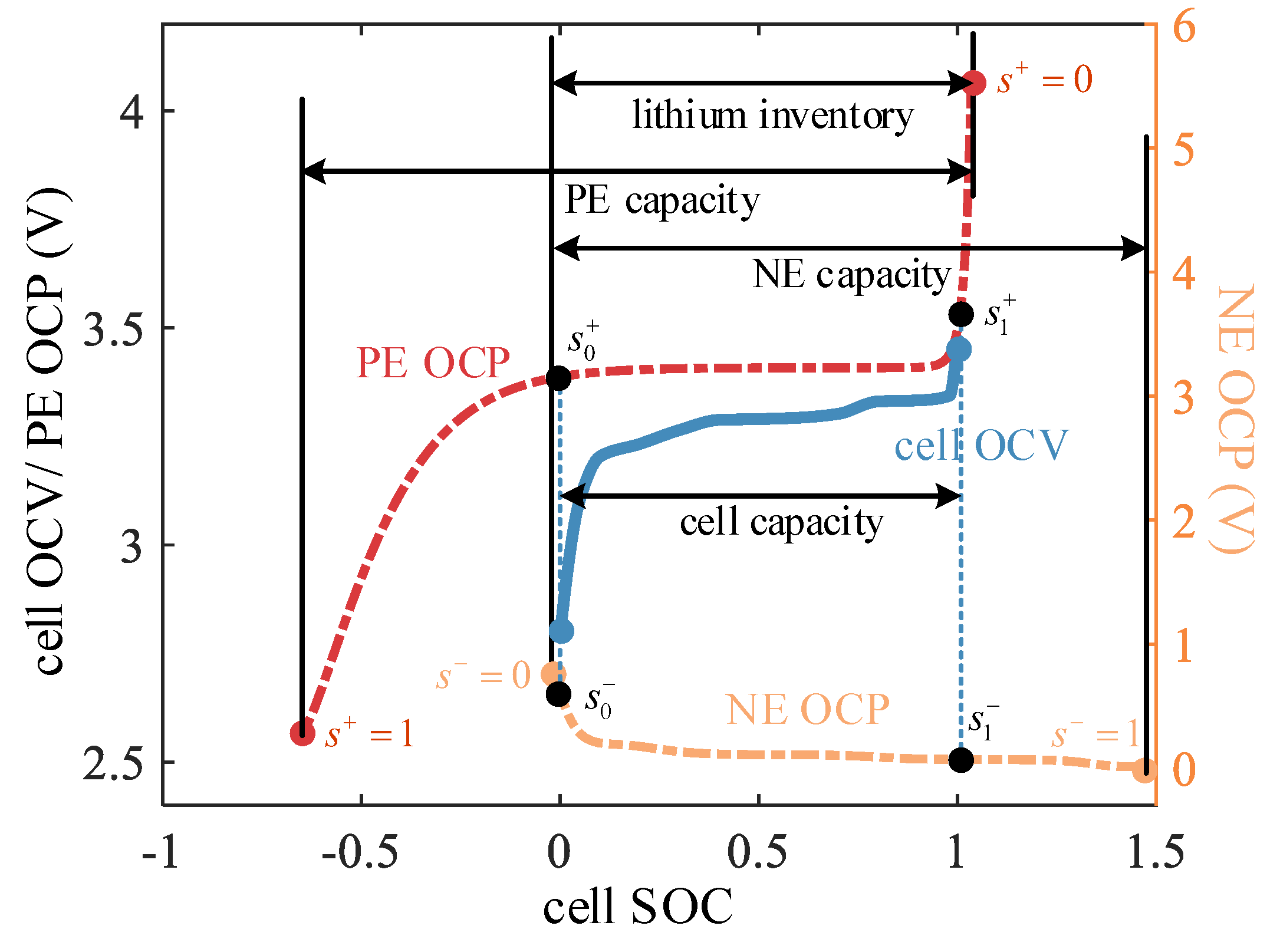
Through the above analysis, the principle of cell OCV reconstruction is shown in Figure 3. denotes the electrode SOC when the cell SOC is equal to 1. Unlike the SOC of the full cell, the electrode SOC () does not vary strictly within 0 to 1, during the full charge and discharge of the cell. The positive and negative electrodes have different electrode SOC ranges, both of which vary as the cell ages and reflect the electrode aging modes. The PE capacity, NE capacity, and lithium inventory are illustrated in Figure 3.

Figure 3.
The principle of cell OCV reconstruction.
Then, the above aging modes can be quantified as follows [22]:
where , , and are corresponding to the three aging modes, respectively. The subscript ’init’ denotes the corresponding value of parameters when the battery is fresh.
3.2. Quantification of Electrode Aging Modes
We expect to quantify battery electrode aging patterns through routine non-invasive characterization tests, including capacity and OCV tests. The key lies in the identification of these electrode aging mechanism parameters, including , , , and . To achieve this, bring Equation (6) into Equation (3), and the following model can be derived:
where Q can be obtained during the cell capacity test. and can be acquired through half-cell OCP tests. During the battery OCV test, can be recorded directly from the sensor, and s can be calculated through capacity test results and working current measurement values.
The parameter identification can be described as the following optimization problem:
where is the measured cell OCV. is the set of parameters to be identified.
Then, based on the OCV test data of the battery, the MPA [31] is used for the identification of the electrode aging mechanism parameters. Considering exploration and exploitation capabilities, MPA mimics the hunting behavior of marine predators with three optimization phases. The phases are equally divided according to the total number of iterations, representing the transition from development to exploration. The main process is as follows: (1) Update the best loss and Elite matrix, and record the Prey matrix. (2) Perform three phases of optimization. (3) Update the best loss and Elite matrix, and record the Prey matrix. (4) Apply the FAD effect and update the Prey matrix. The pseudocode of MPA for parameter identification is shown in Algorithm 1. and are lower and upper bounds of the parameters, respectively. i and n are the index and number of search agents, respectively. records the optimal loss value. and are the current and the latest loss values, respectively. denotes the Prey matrix. is the Elite matrix, which is constructed by the optimal search agent in . k and are the current and maximum iteration, respectively. is the loss function. is a random vector uniformly distributed in the interval . and are random vectors that obey the standard normal distribution and the Lévy distribution, respectively. The notation ⊗ indicates the entry-wise multiplication. denotes the step size adjustment parameter. follows a 0–1 distribution with probability (1-FADS). r is a random vector uniformly distributed in the interval . and are random integers in the range 1 to n.
| Algorithm 1 The pseudocode of MPA for parameter identification. |
Initialization: , , , , , ,
|
Taking fresh cell 1 as an example. The OCV-SOC lookup table is listed in Table 6. Figure 4 shows the results of the reconfiguration of the cell OCV. For better presentation, the measured discrete OCV points (Measured OCV) are interpolated into curves (Inter OCV) with the piecewise cubic hermite interpolating polynomial (PCHIP) method. The fitted OCV curve is the result of the reconstruction based on the identified parameters. The RMSE and MAPE of the fitted OCV and measured OCV are 0.016 V and 0.374%, respectively.

Table 6.
The OCV-SOC lookup table (fresh cell 1).

Figure 4.
Theresult of cell OCV reconstruction (fresh cell 1): (a) OCV curves; (b) OCV error curve.
4. Aging Factor Analysis
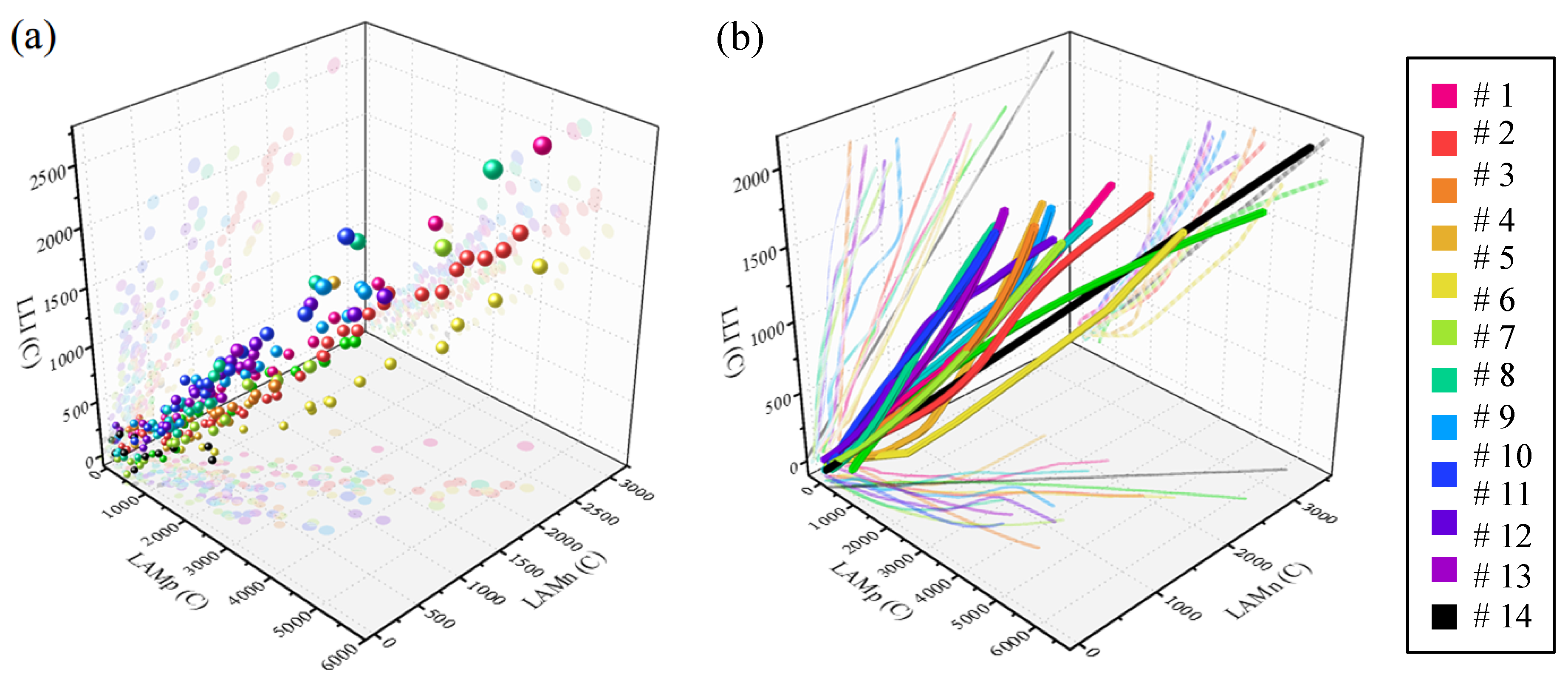
After the above analysis, the capacity decay and aging pattern change law of the battery in the whole life cycle can be obtained. The battery aging paths under different aging conditions can be obtained based on orthogonal experiments, as shown in Figure 5. The size of the sphere indicates the degree of capacity loss. The larger the sphere, the greater the capacity loss. The aging path of all cells under different aging conditions starts close to the origin and ends far from the origin. However, the aging modes have different paths and different path endpoints (end of life) where the capacity decays by 20%. The aging modes of the battery collectively determine capacity decay. The dominance of aging modes affecting battery capacity decay differs under various aging conditions during the whole life cycle. Exploring the effects of aging factors on battery modes can provide more insight into the influence mechanism of aging factors on battery capacity degradation. Therefore, in addition to analyzing the influence of aging factors on battery capacity decay, the effects of each factor on battery aging patterns are further analyzed in this paper.
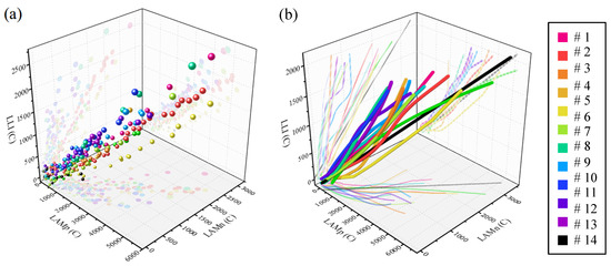
Figure 5.
Battery aging pathways under different aging conditions: (a) scatter plots of measured values under different aging cycles; (b) three-dimensional fitting plots of aging paths.
4.1. Aging Assessment Metrics
First, the indicators to assess battery aging need to be clearly defined. Based on the discussion above, the evaluation indicators (EIs) include capacity degradation (Qloss), LAMp, LAMn, and LLI. Generally, the Ah throughput (equivalent cycles) of a battery over its full life cycle is of great concern. To further analyze the variation of the factors influence degree on battery aging in different aging stages, the life span is divided into pre, mid, and post phases. Then, the ratio of equivalent cycle numbers and the change of EI until a certain phase is considered as the average metric to capture the overall battery aging rate. In addition, the ratio of equivalent cycle numbers and the change of EI within each phase is used as the phase metric to indicate the battery aging rate during different life phases. The specific assessment metrics are defined as follows:
where , , and are the average metrics in pre, mid, and post phases, respectively. , , and are the phase metrics in pre, mid, and post phases, respectively. d denotes the index of EI. , , are the EI values until pre, mid, and post phases, respectively. , , are the changes of EIs within pre, mid, and post phases, respectively. , , and are the cumulative number of equivalent cycles until pre, mid, and post phases, respectively. , , and are the number of equivalent cycles within pre, mid, and post phases, respectively. Generally, the larger these metrics are, the slower the battery ages.
4.2. Analysis of Range
The ANOR method [32] is taken to determine the importance of factors by the range of influence of each factor on the battery aging rate. If j and i denote the indices of factors and levels, respectively, the effect of factor j with level i on the battery aging rate can be calculated as follows:
where is the sum of the experimental responses when factor j is at level i. denotes the times of experiments when factor j is at level i. Then, the influence degree of a factor j on battery aging rate can be expressed as the effect range of factor j at different levels, that is:
A larger indicates a greater influence of factor j on battery aging rate.
4.3. Analysis of Variance
Although ANOR can compare the magnitude of the effect of each factor on the battery aging rate, it cannot indicate which factors are critical or determine whether the effect is significant. In addition, the influence of experimental error is ignored in ANOR. To compensate for these deficiencies, the ANOVA method [33] is used. This method decomposes the fluctuations in the experimental responses into those caused by changes in factor levels and those caused by experimental error. Since there are several stress factors affecting battery aging, the multi-way ANOVA is performed here.
The sum of the squares of deviations of the total responses and factors are defined as follows:
where is the total number of experiments. denotes the experimental response. is the sum of responses. J and I are the number of factors and levels, respectively. According to the design of experiments, C, J, and I are 14, 5, and 3, respectively. Then, the sum of squared deviations of the experimental error can be calculated as follows:
The degree of freedom (DOF) for each factor and error is calculated as follows:
where is the DOF for the total experiment. Then, the mean squares of the deviations of factors and experimental error are defined as follows:
The F value of the Fisher test for each factor can be obtained through . Then, the P-value () can be derived through the calculation of the upper tail of the F cumulative distribution function, which implies that there is a probability of that the change in the experimental responses at different levels of factor j is due to experimental error. In other words, there is a probability that factor j can be considered to have a significant effect on the experimental response (aging rate).
5. Degradation Pathway Prediction Model
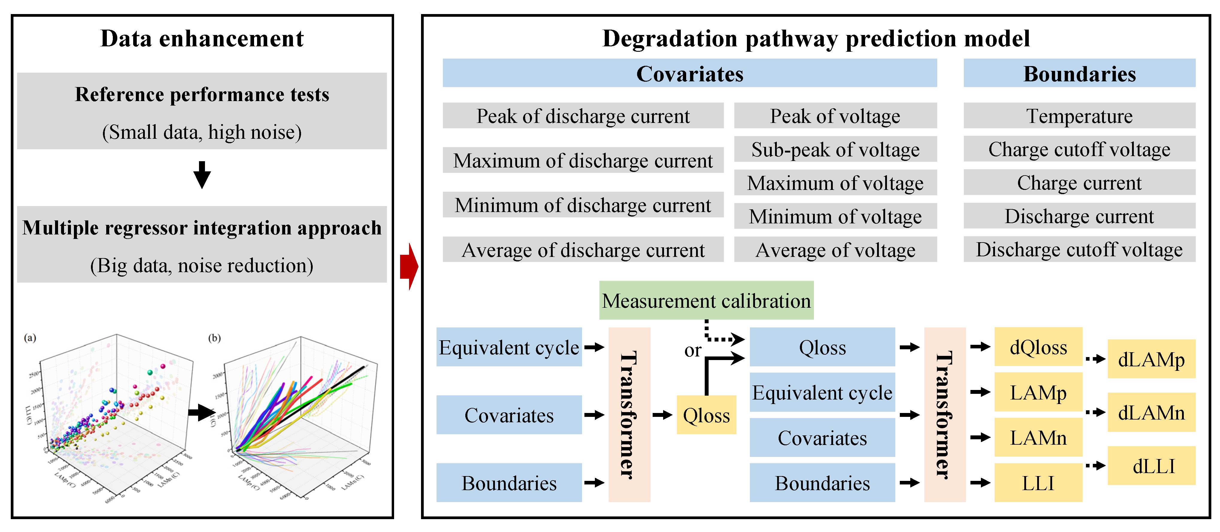
The above analysis is based on the available experimental results. The critical external factors affecting the battery capacity decay, and internal aging modes can be obtained, which can guide battery health management. However, it is not yet possible to achieve fine-grained battery control because the battery degradation pathway under unknown operating conditions is not available. To solve this problem, it is necessary to develop degradation path prediction models. The structure of the degradation pathway prediction model is shown in Figure 6.
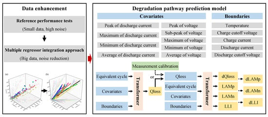
Figure 6.
Structureof the degradation pathway prediction model.
5.1. Regression-Based Data Enhancement
A large amount of effective battery aging data helps in the development of the model. The data needed to quantify the aging pattern comes from reference performance tests. However, the reference performance test is conducted every few hundred charge/discharge cycles, and the amount of data are not sufficient for model training. In addition, these data often contain large amounts of noise, which is not conducive to model development. Therefore, a regression-based data enhancement method is proposed here. The degradation patterns of batteries under different aging conditions are diverse, so it is not appropriate to use a single regression method for data enhancement for different aging condition data. With the idea of ensemble learning, a multiple regressor integration approach is employed. This approach integrates three methods: support vector regression (SVR), neural network (NN), and Gaussian process regression (GPR), and then takes a weighted average of each regression result as the final data augmentation result. In addition, the parameters of the individual regressor are optimized in order to further optimize its performance. The parameters and methods of optimization are shown in Table 7. The optimizer for hyperparameters uses Bayesian optimization and random research. The number of iterations is set to 30. Commonly used hyperparameter tuning methods include grid search, random search, and Bayesian optimization, etc. Grid search is simple but consumes a large amount of computational resources when there are many hyperparameters. Random search, which samples randomly over a range of parameters, is generally more efficient than grid search, but also tends to miss the global optimum. Bayesian optimization is based on Gaussian process and Bayesian theory, and is more efficient and robust than grid search and random search. In this study, Bayesian optimization is mainly used, while random search is used as an auxiliary tool in case the Bayesian optimization results are unsatisfactory. In practice, Bayesian optimization usually gives better results than random search. The kernel function of Bayesian optimization is the automatic relevance determination (ARD) Matern 5/2 kernel [34]:
where and are D-by-1 vectors. and are dth elements of and , respectively. is the signal standard deviation. is the separate length scale for each predictor d. The acquisition function of Bayesian optimization is the expected improvement per second considering overexploiting:
where x denotes the hyperparameter location, and f is the objective function. is the location of the lowest posterior mean of the objective function . is the posterior mean of the evaluation time. If the standard deviation of the posterior objective function is less than 0.5, it is considered to be trapped in a local optimum. In this case, the kernel of the acquisition function is modified to improve the variance of the observations [35]. In order to reduce overfitting and obtain reliable and stable regression results, five-fold cross validation is used.

Table 7.
Theparameters of the multiple regressor integration approach.
Take the relationship between SOH and equivalent cycle of cell 1 as an example. The hyperparameters and results for multiple regression integration are listed in Table 8. The RMSE is used as the regressor performance evaluation metric. Three weight strategies are compared, including 0-1, average and inverse strategies. The 0-1 strategy is to set the weight of the regressor with the lowest RMSE to 1 and the weights of the other regressors to 0. The average strategy is to set all regressor weights to be the same. The inverse strategy assigns weights in proportion to the inverse of the RMSE of individual regressors. The comparative results of multiple regression methods are shown in Figure 7. We can find that the simple 0-1 strategy gives the most desirable performance. Therefore, the 0-1 strategy is adopted in this study.

Table 8.
Hyperparametersand results for multiple regression integration (take the relationship between SOH and equivalent cycle of cell 1 as an example).

Figure 7.
Comparativeresults of multiple regression methods (take the relationship between SOH and equivalent cycle of cell 1 as an example): (a) SOH curves; (b) SOH error curves.
5.2. Transformer-Based Prediction Model
5.2.1. Model Inputs and Outputs
For the model to have excellent performance under different aging conditions, it is necessary to extract enough information from the aging conditions as input to the model. The inputs to the model include three types of data: boundaries, covariates, and independent variables. The constraints consist of five aging factors that limit the operating conditions of the battery. The covariates reflect the statistical characteristics of the voltage and current during the operation of the battery, which can be obtained from historical operating data. The detailed covariates are shown in Figure 6. The independent variables are time-series data, including the number of equivalent cycles and capacity decay.
The battery aging pathway is the curve of the aging modes as the capacity decays under a certain aging condition. Therefore, the outputs of the battery aging pathway prediction model includes the EIs of battery aging (Qloss, LAMp, LAMn, LLI). In addition, to further investigate the effect of different aging factors on the rate of change of EIs, the change of Qloss of two adjacent cycles (dQloss) was also taken as an output. The LAMp, LAMn, and LLI of the next cycle can be predicted by taking dQloss+Qloss as input. These values are then subtracted from the values of the aging modes of the current cycle, and the change in the aging modes (dLAMp, dLAMn, dLLI) of the two adjacent cycles can be obtained. The prediction of the trend of EIs under different aging conditions is significant for future real-time health management. In the process of prediction using the model, if the real capacity decay value is not obtained, the predicted value of capacity decay is generated by the capacity decay prediction model, and then it is used as input for the prediction of aging modes and capacity decay changes. If the current capacity decay value is obtained by measurement, it is used as a measurement calibration to replace the value predicted by the model.
5.2.2. Model Structure
The proposed Transformer model incorporates LSTM, attention mechanism, and gating mechanism. The structure of the hidden layers of the Transformer model is described in detail here. The hidden layers contain three layers: filter layer, encoder–decoder layer, and attention layer.
As can be seen from the previous analysis, there are many inputs to the model. However, since the relationship between the inputs and outputs is unknown in advance, the validity of the inputs cannot be guaranteed and some of them may be harmful to model development. Here, a filtering layer is designed based on the gating mechanism to filter the valid inputs. The gated residual network (GRN) [36] is used to perform the gating mechanism. The filtered constraints and covariates are further used as aging information to generate optional inputs for GRNs:
where is the filtered constraints and covariates. is the optional input. is the optional input when filtering the independent variables. and are initial cell and hidden states for LSTM units in the encoder–decoder layer. is the optional input of the attention layer. Then, the filter layer output is calculated as follows:
where is the independent variable input. is the filtering weight that is calculated through the softmax operation:
In the temporal prediction task, an encoder–decoder layer is designed in order to establish the relationship between historical information and future trends. This layer is based on LSTM units [37]. For the sake of simplicity, the numbers of both encoders and decoders are set to 1. and are input to this layer as the initial cell and hidden states of the LSTM unit.
After the filtering and encoder–decoder layers comes the attention layer. Long-term and short-term dependencies are learned using a multi-headed attention mechanism. The attention is defined as follows [38]:
where , , and are value, query, and key, respectively. d is the dimension. is the mask matrix. Through sharing values in each head, multi-head attention is designed as follows [36]:
where i and h are the index and number of heads. , , and are weights of value, query, and key for head i. is the linear mapping matrix.
6. Results and Analysis
6.1. Ofat Experimental Analysis
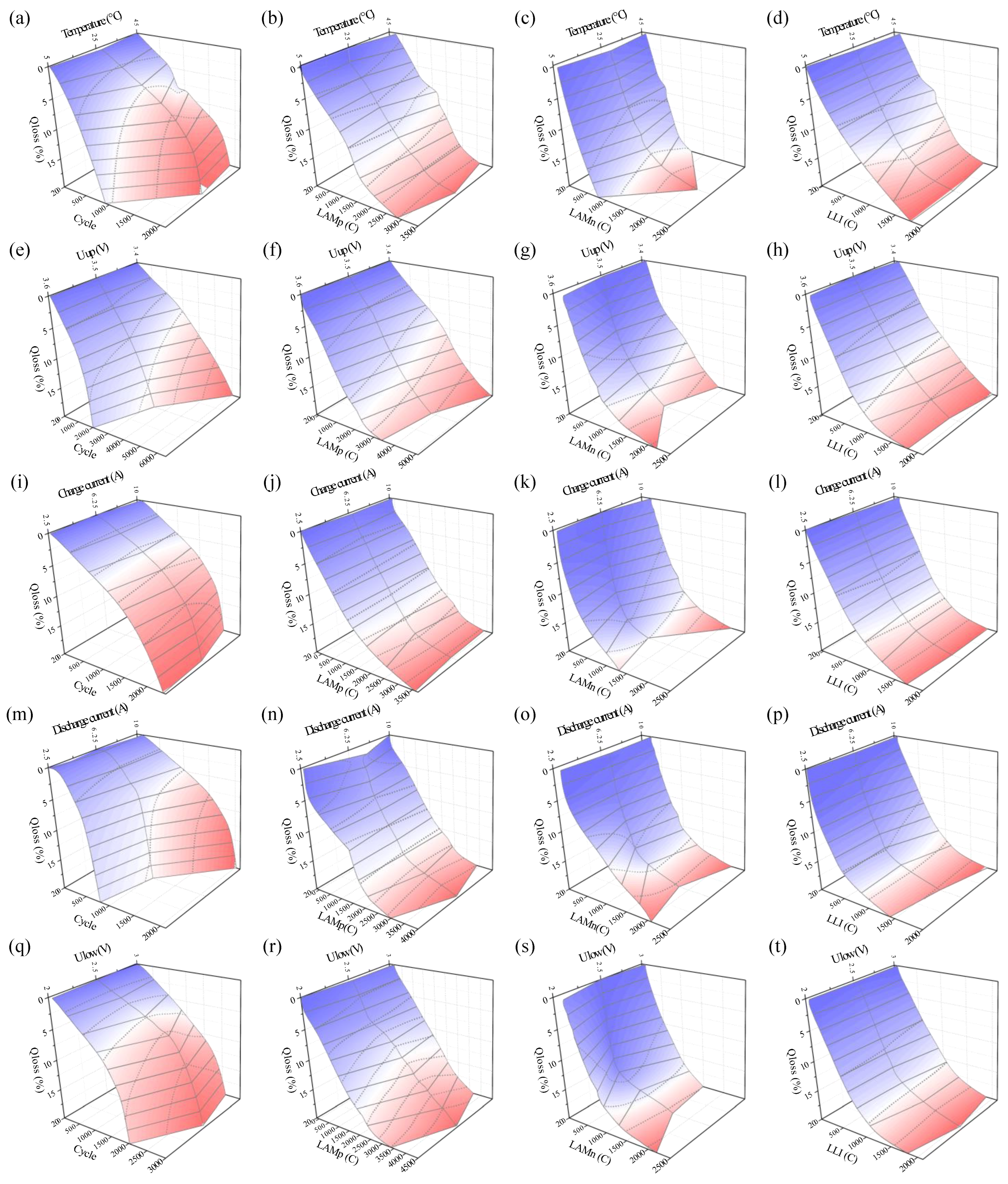
Based on the OFAT experimental results, the effects of the variation of each factor on battery aging are analyzed, as shown in Figure 8. Variations of the profile of capacity decay with the equivalent cycle at different levels of a particular factor are presented in Figure 8a,e,i,m,q. Variations of the profile of aging modes (LAMp, LAMn, LLI) with capacity decay at different levels of a particular factor are presented in Figure 8b,f,j,n,r, Figure 8c,g,k,o,s, and Figure 8d,h,l,p,t, respectively. Taking the aging conditions of cell 1 as a reference, we can see the optimal and worst aging factor levels for capacity decay or for the three aging modes. For example, temperature conditions set to 25 °C will make the battery capacity decay more slowly than 5 °C or 45 °C. At 25 °C, LAMp and LAMn are greater at the battery end of life (capacity loss is equal to 20%) compared to those at 5 °C and 45 °C. This is because the cell has a higher number of equivalent cycles at 25 °C. This means that, under this condition, the positive and negative electrodes are used more efficiently. The variation of LLI at the end of life is not significant at different temperatures. The effects of other factors can be analyzed similarly. It is a guideline for how to change the aging factor level to obtain the battery life extension.
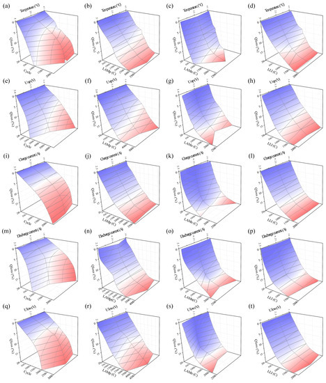
Figure 8.
The effects of the variation of each factor on battery aging: (a–d) Temperature (), (e–h) Charge cutoff voltage (), (i–l) Charge current (), (m–p) Discharge current (), (q–t) Discharge cutoff voltage (); (a,e,i,m,q) Impact on Qloss, (b,f,j,n,r) Impact on LAMp, (c,g,k,o,s) Impact on LAMn, (d,h,l,p,t) Impact on LLI.
6.2. Results of the Analysis of Range
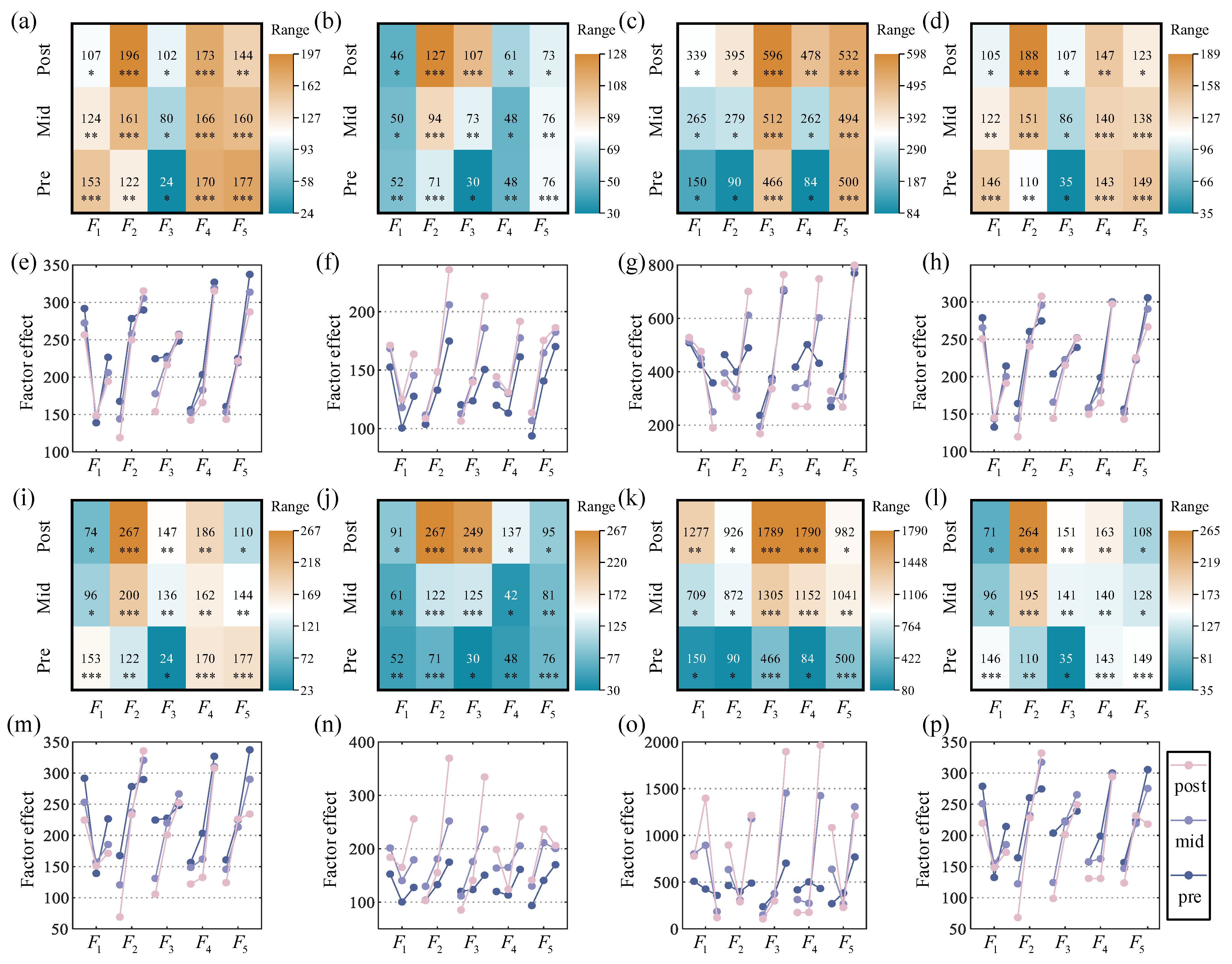
The ANOR results of battery degradation can be obtained as shown in Figure 9. Each heat map represents the degree of influence of five factors (–) on a particular EI at three aging phases (pre, mid, and post phases), where EI includes Qloss, LAMp, LAMn, and LLI, and the metric of influence includes average metrics and phase metrics. For the convenience of the analysis, the results of ANOR values for the same aging metrics at the same phase for the five factors (each row) are divided equally into three levels and indicated by stars (large: , medium: , and small: ). Overall, the degree of influence of the factors on the capacity decay and aging modes of the battery varies in different aging phases. The effects of factors on Qloss and LLI are strongly consistent across different phases of the full life cycle. This may be due to the apparent linear relationship between Qloss and LLI. During the full life cycle, Temperature () has little effect on LAMp and LAMn, and the effects on Qloss and LLI are greater in the pre phase of aging and smaller in the post phase of aging. Charge cutoff voltage () has a large effect on Qloss, LAMp, and LLI, but a small effect on LAMn. The effect of charge current () on Qloss and LLI is small, but the effect on LAMn is relatively large, and the effect on LAMp is larger in the mid and post aging phases. The impact of discharge current () on Qloss and LLI is large over the full life cycle, but the impact on LAMp is not significant. The effect on LAMn is small in the pre phase and larger in the post stage. The effect of discharge cutoff voltage () on LAMn is always significant, and the effect on LLI and capacity decay is also great, but decreases with life, as is the effect on LAMp. Throughout the life cycle, the factors that have a large impact on Qloss are , , and . The LAMp is strongly influenced by the factors and . The LAMn is greatly affected by the factors , , and . The LLI is mainly influenced by factors and .
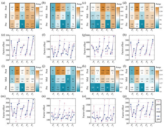
Figure 9.
The ANOR results of battery degradation: (a–h) average metrics, (i–p) phase metrics; (a,e,i,m) EI is Qloss, (b,f,j,n) EI is LAMp, (c,g,k,o) EI is LAMn, (d,h,l,p) EI is LAMp; (a–d,i–l) the influence degree of the factor j on battery aging rate (), (e–h,m–p) the effect of factor j with level i on battery aging rate (). The ANOR values are divided equally into three levels and indicated by stars (large: , medium: , and small: ).
In addition, the factor effects at different levels on the battery aging rate () are also presented in Figure 9. The lighter the color of the curve, the more posterior the aging. The larger the value of the curve, the slower the battery aging rate at that level of the factor. We can find that there is a certain rule for the effect of different levels of factors on capacity decay and aging modes in different aging phases. Then, we can derive the best and worst combinations of factor levels that affect the battery aging rate (EIs), as shown in Table 9. In general, the milder the aging conditions, the slower the rate of battery aging. The harsher the aging conditions, the faster the rate of battery aging. However, there is a slight discrepancy in the ANOR results of the orthogonal experiments. The exceptions are bolded in the table. The accelerating effect of low temperature (5 °C) on LAMn aging is more obvious than that of high temperature (45 °C). However, low temperature (5 °C) has a greater accelerating effect on Qloss, LAMp, and LLI than high temperature (45 °C). For the worst combination of factor levels of LAMp and LAMn, the discharge current is 6.25 A, not 10 A. In addition, the worst voltage operating interval for LAMn is 2.5–3.5 V, not 2.0–3.6 V. The reason for this is that the voltage operating range and current magnitude will determine the Ah throughput and operating time of a charge/discharge cycle. The narrower the voltage range and the lower the current, the lower the Ah throughput per unit time and the longer the operation time will be. This will exacerbate the effects of calendar aging on accelerated cycle aging.

Table 9.
The best and worst combinations of factor levels that affect the battery aging rate.
6.3. Results of the Analysis of Variance
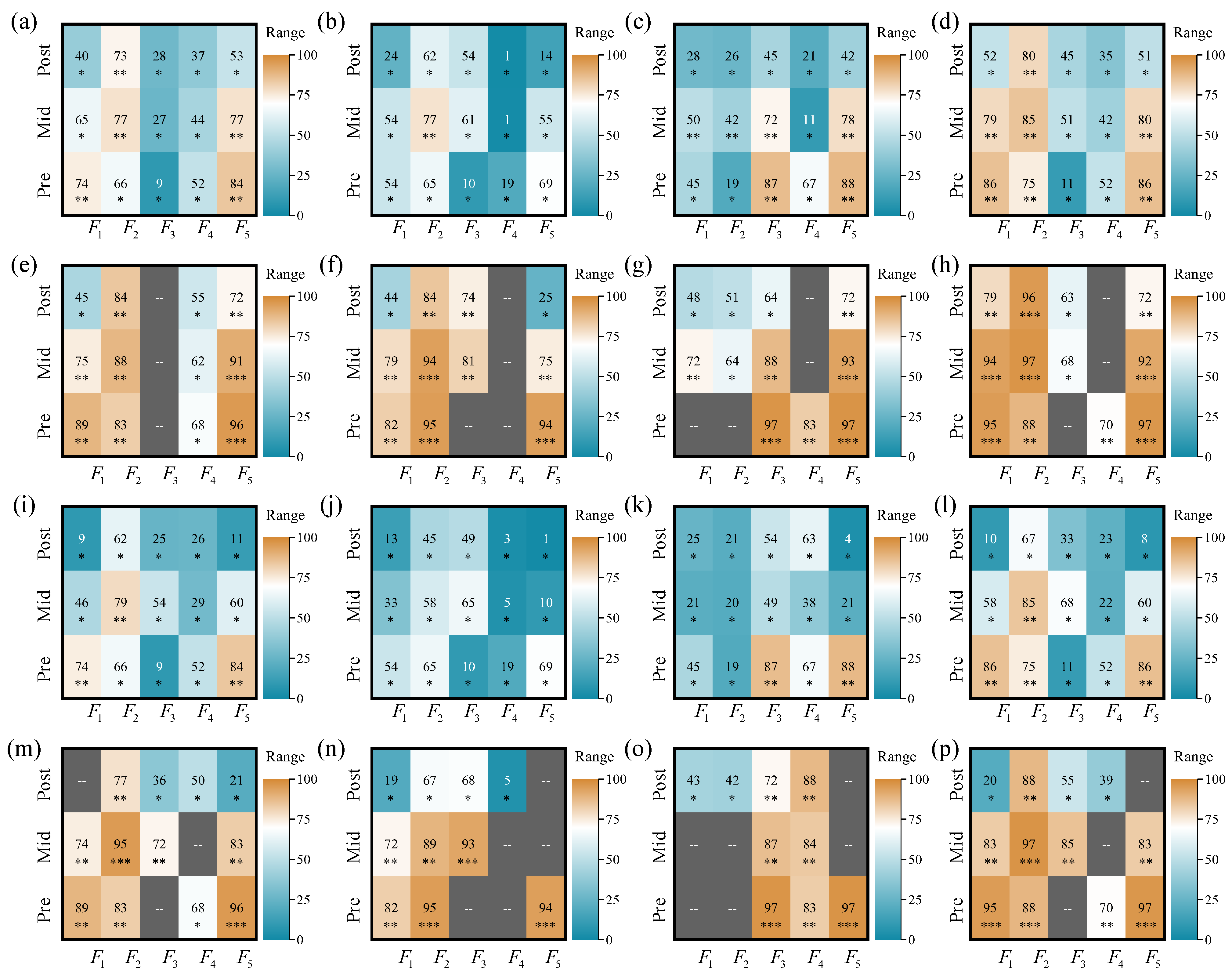
The ANOVA results of battery degradation are shown in Figure 10. Each heat map represents the values of five factors (–) on a particular EI at three aging phases. The metric of influence includes average metrics and phase metrics. To improve the reliability of the ANOVA results, if the of the factor j is less than the , this factor j is considered negligible and incorporated into the experimental error. Then, the ANOVA is performed again. The corresponding heat map is filled with gray. For analysis convenience, the results of ANOVA significance analysis are divided into different levels (negligible: , insignificant (<70): ∗, relatively significant (70–90): , significant (>90): ). In general, the significance of each factor on the battery capacity decay and aging modes varies at different aging phases. Temperature () has the most significant effect on LLI, followed by Qloss and LAMp, and the least significant effect on LAMn. Charge cutoff voltage () has a significant effect on Qloss, LAMp, and LLI, but an insignificant or negligible effect on LAMn. Charge current () has a certain degree of effect on LAMp and LAMn, but the effect on Qloss and LLI is insignificant or negligible. The effects of discharge current () on Qloss, LAMp, LAMn, and LLI are not very significant. Different from , the effects of discharge cutoff voltage () on both capacity decay and aging modes are quite significant, but the significance decreases as the battery ages. During the whole life cycle, the factors that have a large impact on Qloss are and . The LAMp is greatly influenced by the factors and . The LAMn is strongly affected by the factor . The LLI is mainly impacted by factors , , and . We can find that the results of ANOR and ANOVA are generally consistent, except for a slight difference. The reason is that the former is analyzed from the perspective of range, and the latter is analyzed from the point of view of variance.
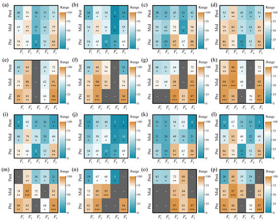
Figure 10.
The ANOVA results of battery degradation: (a–h) average metrics, (i–p) phase metrics; (a,e,i,m) EI is Qloss, (b,f,j,n) EI is LAMp, (c,g,k,o) EI is LAMn, (d,h,l,p) EI is LAMp; (a–d,i–l) results of full factors analysis, (e–h,m–p) Results of refined factors analysis. The results of ANOVA are divided into different levels (negligible: , insignificant (<70): ∗, relatively significant (70–90): , significant (>90): ).
6.4. Analysis of Dominant Aging Modes
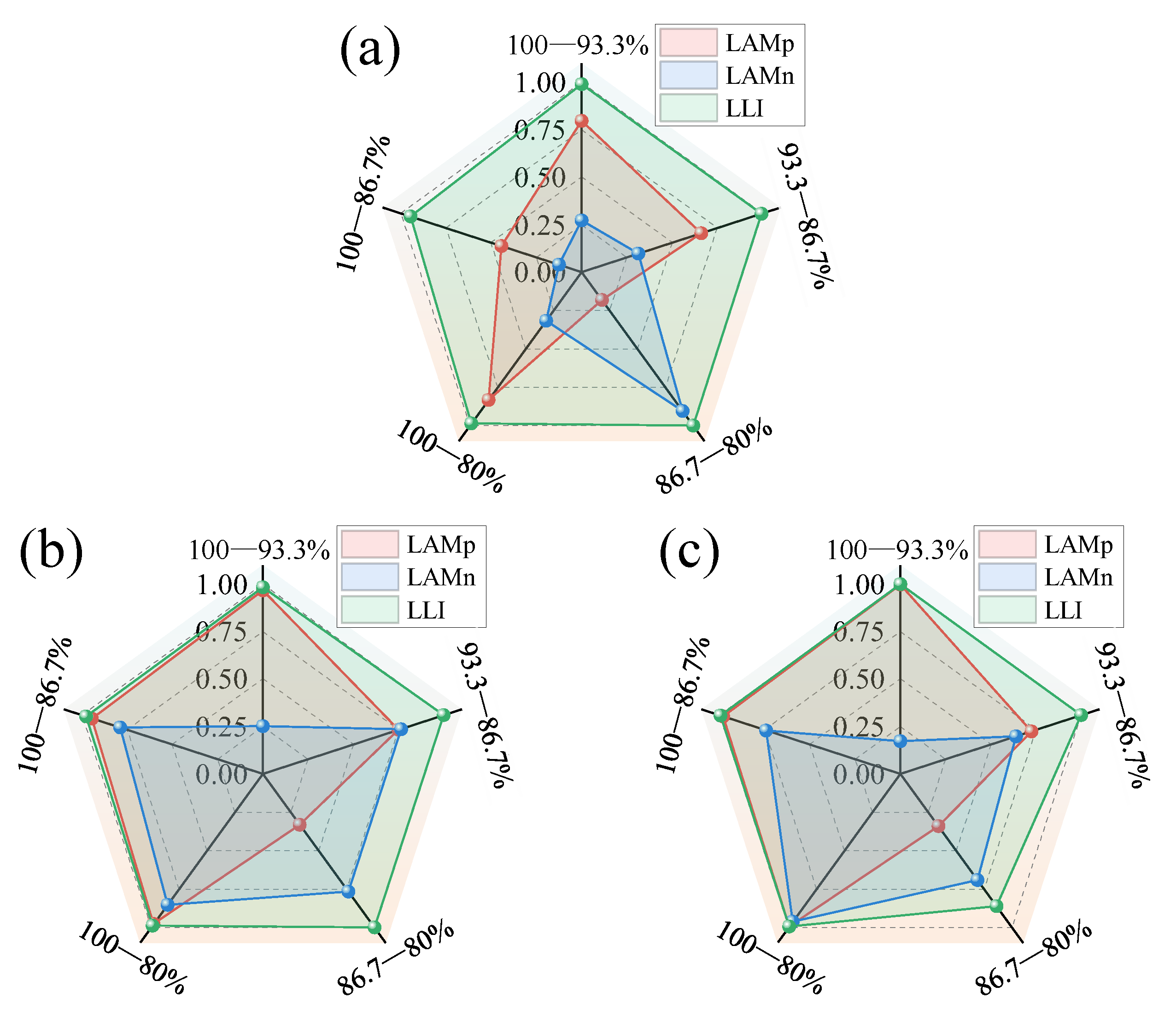
The critical factors affecting battery aging are analyzed above by ANOR and ANOVA in terms of range and variance, respectively. On this basis, the dominant aging modes for capacity attenuation at different aging phases can be derived. By calculating the Pearson correlation of the ANOR/ANOVA result matrix of each aging mode with that of capacity decay, the dominant aging mode can be deduced. The results are presented in the form of a radar plot, as shown in Figure 11. The value of the correlation coefficient is linearly transformed to the value between 0 and 1 as an evaluation indicator of dominance that is ( + 1)/2. The axes represent the different aging phases. We can find that the LLI has the largest area in all three subplots and is close to 1 on each axis. This means that both ANOR and ANOVA analyses lead to the consistent conclusion that LLI is the dominant aging mode for battery capacity decay at different aging phases. From the results of the ANOVA analysis, it can be obtained that LAMp is also dominant in the aging phases of 100–93.3%, 100–86.7%, and 100–80%. Meanwhile, we can see the presence of non-dominant aging modes in certain aging stages, such as LAMn in the 100–93.3% aging phase.
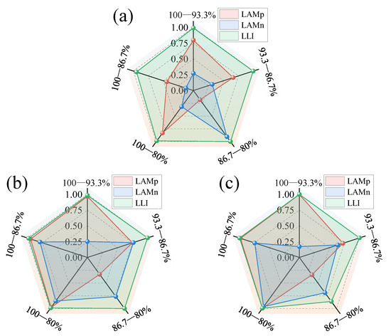
Figure 11.
Analysis of dominant aging mode of capacity attenuation: (a) ANOR results; (b) Full factors ANOVA results; (c) Refined factors’ ANOVA results.
6.5. Prediction Model Performance Validation
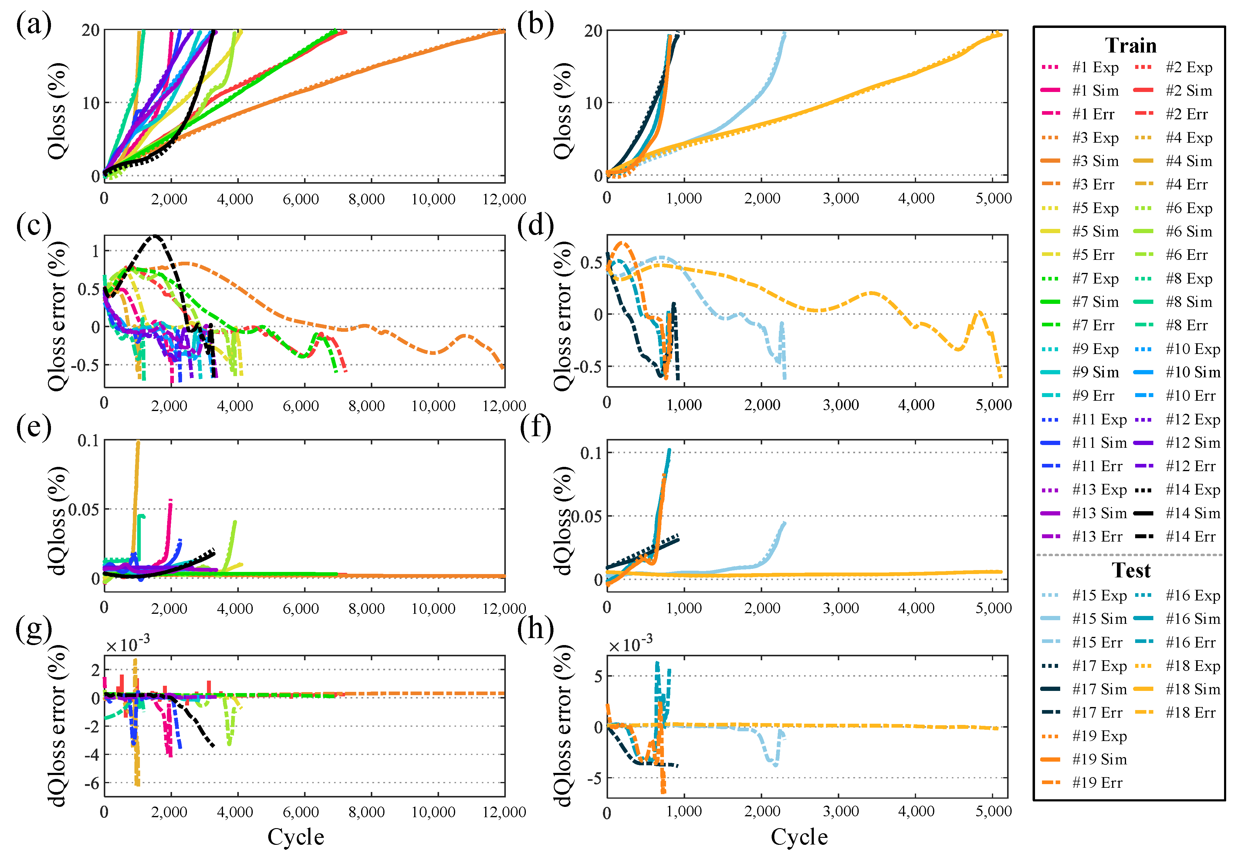
The data of 14 cells from the orthogonal experiments are used as the training set (cell 1–cell 14) to train the degradation pathway prediction model. The data of cells with different aging conditions from these 14 cells are selected as the test set (cell 15–cell 19) to verify the aging condition generalization of the established prediction model. The performance of prediction models for capacity decay (Qloss) and its rate of change (dQloss) is shown in Figure 12. We can see that the capacity decay curves and capacity decay change rate curves of batteries under different aging conditions are very diverse. Some cells show an approximately linear change in capacity decay with increasing equivalent cycles during the whole life cycle, such as cell 4 and cell 7. Some cells show approximately linear changes in capacity decay with equivalent cycles in the early phase but a significant acceleration in decay rate in the later phase, such as cell 8 and cell 15. However, the model achieves excellent prediction accuracy regardless of the pattern of variation. The error of the model predicted capacity decay and its rate of change on the test set can be guaranteed to be within ±0.7% and ±0.0007%, respectively.
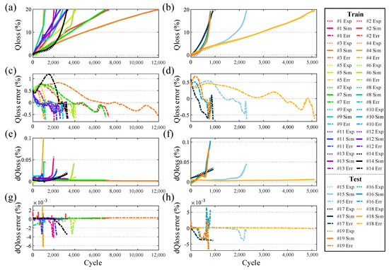
Figure 12.
Performance of prediction models for capacity decay (Qloss) and its rate of change (dQloss): (a) Training outputs for Qloss; (b) Test outputs for Qloss; (c) Training errors for Qloss; (d) Test errors for Qloss; (e) Training outputs for dQloss; (f) Test outputs for dQloss; (g) Training errors for dQloss; (h) Test errors for dQloss.
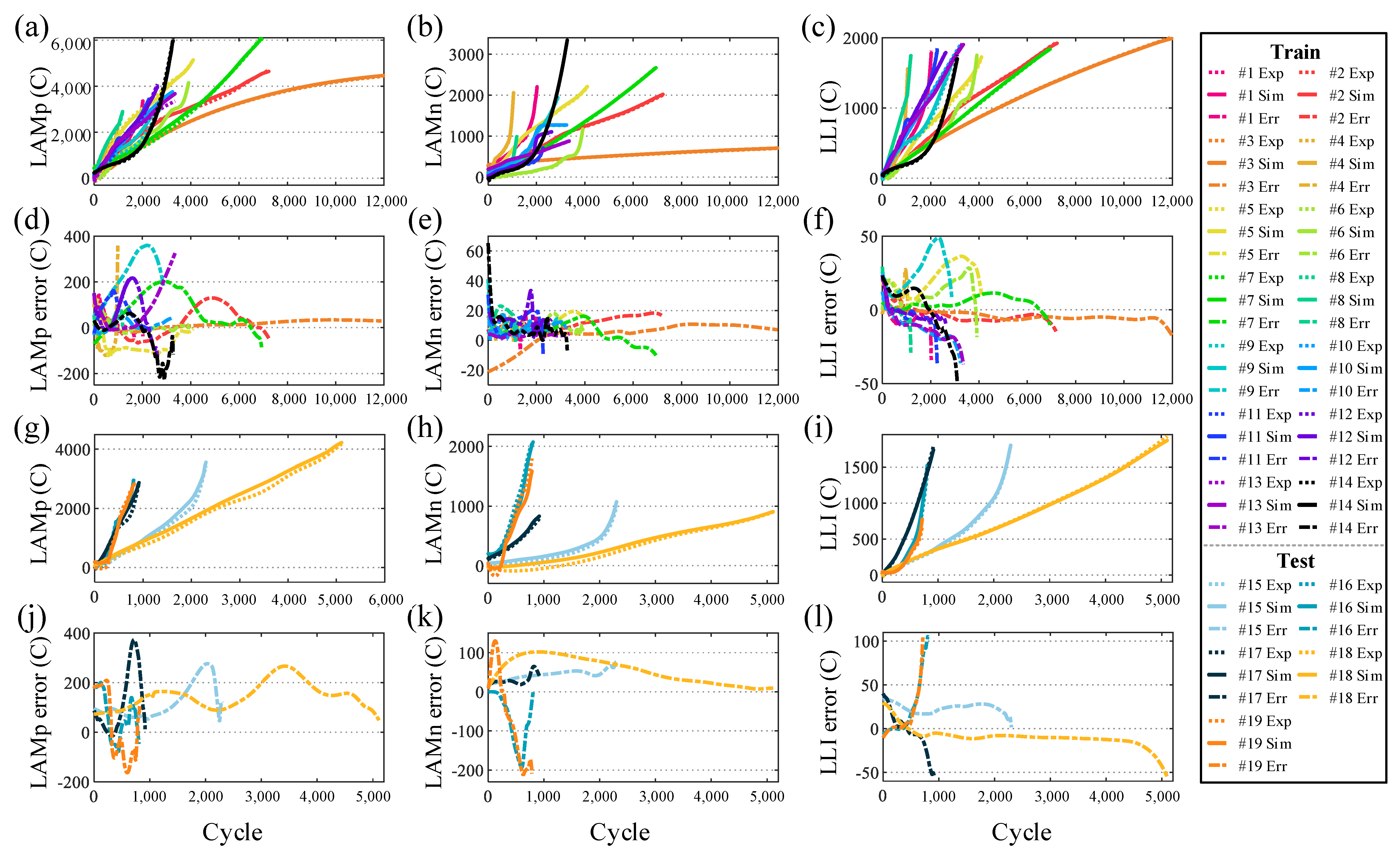
The performance of prediction models for three aging modes (LAMp, LAMn, and LLI) is shown in Figure 13. We can find that the variation patterns of Qloss with equivalent cycles for all cells are very similar to those of LLI. The change patterns of the three aging modes in the whole life cycle under various aging conditions are different. The prediction errors of LAMp, LAMn, and LLI of the model on the test set can be maintained within −200–400 C, −200–150 C, and −50–100 C, respectively. The numerical results of model prediction errors are listed in Table 10. Root mean square error (RMSE), mean absolute error (MAE), mean absolute percentage error (MAPE), and R-square value are statistically calculated. This indicates that the established aging trajectory prediction model has excellent prediction performance.
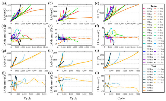
Figure 13.
Performance of prediction models for three aging modes: (a–d) LAMp prediction results, (e–h) LAMn prediction results, (i–l) LLI prediction results; (a,e,i) Training outputs for aging modes, (b,f,j) Training errors for aging modes, (c,g,k) Test outputs for aging modes, (d,h,l) Test errors for aging modes.

Table 10.
Numericalresults of model prediction errors.
7. Conclusions
In this paper, a data-driven method is proposed to analyze the internal aging mechanism and predict the degradation path of lithium-ion batteries. The OCV reconfiguration model is established to achieve a non-destructive quantitative study of the aging mechanism, and the MPA is developed for the identification of aging mechanism parameters. The multi-factor and multi-level orthogonal aging experiments of the batteries are carefully designed and performed to investigate the critical aging factors and dominant aging modes at different aging phases under different aging conditions. On this basis, the effects of different factors on battery aging are quantified using ANOR and ANOVA methods, and the dominant aging modes of capacity decay are determined using correlation analysis methods. In addition, a Transformer-based capacity decay and aging modes pathway prediction model is proposed, and a data enhancement technique based on a multiple regression integration method is designed to empower the Transformer model. The experimental results show that the proposed method can obtain excellent prediction accuracy under unknown aging conditions with R-squared values greater than 0.98.
We find that the influence degree of factors (temperature, charge cutoff voltage, charge current, discharge current, discharge cutoff voltage) on battery aging (Qloss, LAMp, LAMn, and LLI) varies in different aging phases. The best and worst combinations of different aging factor levels are analyzed, which guides how factors can be changed to extend battery life. The battery capacity decay is essentially determined by a combination of LAMp, LAMn, and LLI aging modes. However, the LLI is always the dominant aging mode throughout the whole life cycle, whether evaluated in terms of average or phase capacity decay. The LAMp is also dominant if average capacity decay is used as an evaluation metric. The Transformer model provides accurate predictions of battery capacity decay and aging modes under different factors, providing the basis for in-depth battery health management in the future.
Author Contributions
Conceptualization, methodology, software, writing—original draft preparation, visualization, data curation, R.X.; writing—review and editing, investigation, supervision, resources, validation, funding acquisition, Y.W.; writing—review and editing, formal analysis, project administration, funding acquisition, Z.C. All authors have read and agreed to the published version of the manuscript.
Funding
This work was supported by the National Natural Science Fund of China (Grant Nos. 91848111, 61803359), and the Natural Science Foundation of Anhui Province (Grant No. 2208085UD12).
Data Availability Statement
The data that support the findings of this study are available from the corresponding author upon reasonable request.
Conflicts of Interest
The authors declare no conflict of interest.
References
- Wang, Y.; Xu, R.; Zhou, C.; Kang, X.; Chen, Z. Digital twin and cloud-side-end collaboration for intelligent battery management system. J. Manuf. Syst. 2022, 62, 124–134. [Google Scholar] [CrossRef]
- Severson, K.A.; Attia, P.M.; Jin, N.; Perkins, N.; Jiang, B.; Yang, Z.; Chen, M.H.; Aykol, M.; Herring, P.K.; Fraggedakis, D.; et al. Data-driven prediction of battery cycle life before capacity degradation. Nat. Energy 2019, 4, 383–391. [Google Scholar] [CrossRef]
- Wang, Y.; Tian, J.; Sun, Z.; Wang, L.; Xu, R.; Li, M.; Chen, Z. A comprehensive review of battery modeling and state estimation approaches for advanced battery management systems. Renew. Sustain. Energy Rev. 2020, 131, 110015. [Google Scholar] [CrossRef]
- Hu, X.; Xu, L.; Lin, X.; Pecht, M. Battery lifetime prognostics. Joule 2020, 4, 310–346. [Google Scholar] [CrossRef]
- Wang, Y.; Li, K.; Chen, Z. Battery Full Life Cycle Management and Health Prognosis Based on Cloud Service and Broad Learning. IEEE/CAA J. Autom. Sin. 2022, 9, 1540–1542. [Google Scholar] [CrossRef]
- Xu, P.; Hu, X.; Liu, B.; Ouyang, T.; Chen, N. Hierarchical estimation model of state-of-charge and state-of-health for power batteries considering current rate. IEEE Trans. Ind. Inform. 2021, 18, 6150–6159. [Google Scholar] [CrossRef]
- Arrinda, M.; Oyarbide, M.; Macicior, H.; Muxika, E. Unified Evaluation Framework for Stochastic Algorithms Applied to Remaining Useful Life Prognosis Problems. Batteries 2021, 7, 35. [Google Scholar] [CrossRef]
- Li, W.; Rentemeister, M.; Badeda, J.; Jöst, D.; Schulte, D.; Sauer, D.U. Digital twin for battery systems: Cloud battery management system with online state-of-charge and state-of-health estimation. J. Energy Storage 2020, 30, 101557. [Google Scholar] [CrossRef]
- Song, Y.; Peng, Y.; Liu, D. Model-based health diagnosis for lithium-ion battery pack in space applications. IEEE Trans. Ind. Electron. 2020, 68, 12375–12384. [Google Scholar] [CrossRef]
- Tian, J.; Wang, Y.; Chen, Z. An improved single particle model for lithium-ion batteries based on main stress factor compensation. J. Clean. Prod. 2021, 278, 123456. [Google Scholar] [CrossRef]
- Xu, R.; Wang, Y.; Chen, Z. A migration-based method for non-invasive revelation of microscopic degradation mechanisms and health prognosis of lithium-ion batteries. J. Energy Storage 2022, 55, 105769. [Google Scholar] [CrossRef]
- Tian, J.; Xu, R.; Wang, Y.; Chen, Z. Capacity attenuation mechanism modeling and health assessment of lithium-ion batteries. Energy 2021, 221, 119682. [Google Scholar] [CrossRef]
- Tang, X.; Zou, C.; Yao, K.; Lu, J.; Xia, Y.; Gao, F. Aging trajectory prediction for lithium-ion batteries via model migration and Bayesian Monte Carlo method. Appl. Energy 2019, 254, 113591. [Google Scholar] [CrossRef]
- Yang, F.; Song, X.; Dong, G.; Tsui, K.L. A coulombic efficiency-based model for prognostics and health estimation of lithium-ion batteries. Energy 2019, 171, 1173–1182. [Google Scholar] [CrossRef]
- You, H.; Dai, H.; Li, L.; Wei, X.; Han, G. Charging Strategy Optimization at Low Temperatures for Li-Ion Batteries Based on Multi-Factor Coupling Aging Model. IEEE Trans. Veh. Technol. 2021, 70, 11433–11445. [Google Scholar] [CrossRef]
- Yao, Z.; Lum, Y.; Johnston, A.; Mejia-Mendoza, L.M.; Zhou, X.; Wen, Y.; Aspuru-Guzik, A.; Sargent, E.H.; Seh, Z.W. Machine learning for a sustainable energy future. Nat. Rev. Mater. 2022. [Google Scholar] [CrossRef]
- Lv, C.; Zhou, X.; Zhong, L.; Yan, C.; Srinivasan, M.; Seh, Z.W.; Liu, C.; Pan, H.; Li, S.; Wen, Y.; et al. Machine learning: An advanced platform for materials development and state prediction in lithium-ion batteries. Adv. Mater. 2022, 34, 2101474. [Google Scholar] [CrossRef]
- Ren, Z.; Du, C.; Ren, W. State of Health Estimation of Lithium-Ion Batteries Using a Multi-Feature-Extraction Strategy and PSO-NARXNN. Batteries 2023, 9, 7. [Google Scholar] [CrossRef]
- Chahbaz, A.; Meishner, F.; Li, W.; Ünlübayir, C.; Sauer, D.U. Non-invasive identification of calendar and cyclic ageing mechanisms for lithium-titanate-oxide batteries. Energy Storage Mater. 2021, 42, 794–805. [Google Scholar] [CrossRef]
- Birkl, C.R.; Roberts, M.R.; McTurk, E.; Bruce, P.G.; Howey, D.A. Degradation diagnostics for lithium ion cells. J. Power Sources 2017, 341, 373–386. [Google Scholar] [CrossRef]
- Dong, G.; Wei, J. A physics-based aging model for lithium-ion battery with coupled chemical/mechanical degradation mechanisms. Electrochim. Acta 2021, 395, 139133. [Google Scholar] [CrossRef]
- Li, W.; Chen, J.; Quade, K.; Luder, D.; Gong, J.; Sauer, D.U. Battery degradation diagnosis with field data, impedance-based modeling and artificial intelligence. Energy Storage Mater. 2022, 53, 391–403. [Google Scholar] [CrossRef]
- Tian, J.; Xiong, R.; Shen, W.; Sun, F. Electrode ageing estimation and open circuit voltage reconstruction for lithium ion batteries. Energy Storage Mater. 2021, 37, 283–295. [Google Scholar] [CrossRef]
- Dubarry, M.; Beck, D. Big data training data for artificial intelligence-based Li-ion diagnosis and prognosis. J. Power Sources 2020, 479, 228806. [Google Scholar] [CrossRef]
- Farkhondeh, M.; Delacourt, C. Mathematical modeling of commercial LiFePO4 electrodes based on variable solid-state diffusivity. J. Electrochem. Soc. 2011, 159, A177. [Google Scholar] [CrossRef]
- Safari, M.; Delacourt, C. Modeling of a commercial graphite/LiFePO4 cell. J. Electrochem. Soc. 2011, 158, A562. [Google Scholar] [CrossRef]
- Delacourt, C.; Safari, M. Analysis of lithium deinsertion/insertion in LiyFePO4 with a simple mathematical model. Electrochim. Acta 2011, 56, 5222–5229. [Google Scholar] [CrossRef]
- Ding, Q.; Wang, Y.; Chen, Z. Parameter identification of reduced-order electrochemical model simplified by spectral methods and state estimation based on square-root cubature Kalman filter. J. Energy Storage 2022, 46, 103828. [Google Scholar] [CrossRef]
- Jiang, Z.; Zhang, D.; Lu, G. Radial artery pulse waveform analysis based on curve fitting using discrete Fourier series. Comput. Methods Programs Biomed. 2019, 174, 25–31. [Google Scholar] [CrossRef]
- Georgiou, S.D.; Stylianou, S.; Drosou, K.; Koukouvinos, C. Construction of orthogonal and nearly orthogonal designs for computer experiments. Biometrika 2014, 101, 741–747. [Google Scholar] [CrossRef]
- Faramarzi, A.; Heidarinejad, M.; Mirjalili, S.; Gandomi, A.H. Marine Predators Algorithm: A nature-inspired metaheuristic. Expert Syst. Appl. 2020, 152, 113377. [Google Scholar] [CrossRef]
- Su, L.; Zhang, J.; Wang, C.; Zhang, Y.; Li, Z.; Song, Y.; Jin, T.; Ma, Z. Identifying main factors of capacity fading in lithium ion cells using orthogonal design of experiments. Appl. Energy 2016, 163, 201–210. [Google Scholar] [CrossRef]
- Jiaqiang, E.; Han, D.; Qiu, A.; Zhu, H.; Deng, Y.; Chen, J.; Zhao, X.; Zuo, W.; Wang, H.; Chen, J.; et al. Orthogonal experimental design of liquid-cooling structure on the cooling effect of a liquid-cooled battery thermal management system. Appl. Therm. Eng. 2018, 132, 508–520. [Google Scholar]
- Snoek, J.; Larochelle, H.; Adams, R.P. Practical bayesian optimization of machine learning algorithms. In Advances in Neural Information Processing Systems; Curran Associates, Inc.: Red Hook, NY, USA, 2012; Volume 25. [Google Scholar]
- Bull, A.D. Convergence rates of efficient global optimization algorithms. J. Mach. Learn. Res. 2011, 12, 2879–2904. [Google Scholar]
- Lim, B.; Arık, S.Ö.; Loeff, N.; Pfister, T. Temporal fusion transformers for interpretable multi-horizon time series forecasting. Int. J. Forecast. 2021, 37, 1748–1764. [Google Scholar] [CrossRef]
- Li, K.; Wang, Y.; Chen, Z. A comparative study of battery state-of-health estimation based on empirical mode decomposition and neural network. J. Energy Storage 2022, 54, 105333. [Google Scholar] [CrossRef]
- Vaswani, A.; Shazeer, N.; Parmar, N.; Uszkoreit, J.; Jones, L.; Gomez, A.N.; Kaiser, Ł.; Polosukhin, I. Attention is all you need. In Advances in Neural Information Processing Systems; Curran Associates, Inc.: Red Hook, NY, USA, 2017; Volume 30. [Google Scholar]
Disclaimer/Publisher’s Note: The statements, opinions and data contained in all publications are solely those of the individual author(s) and contributor(s) and not of MDPI and/or the editor(s). MDPI and/or the editor(s) disclaim responsibility for any injury to people or property resulting from any ideas, methods, instructions or products referred to in the content. |
© 2023 by the authors. Licensee MDPI, Basel, Switzerland. This article is an open access article distributed under the terms and conditions of the Creative Commons Attribution (CC BY) license (https://creativecommons.org/licenses/by/4.0/).

