
Estimation of Lithium-ion Battery Discharge Capacity by Integrating Optimized Explainable-AI and Stacked LSTM Model

 ,
,  ,
,  ,
, 

Abstract
:1. Introduction
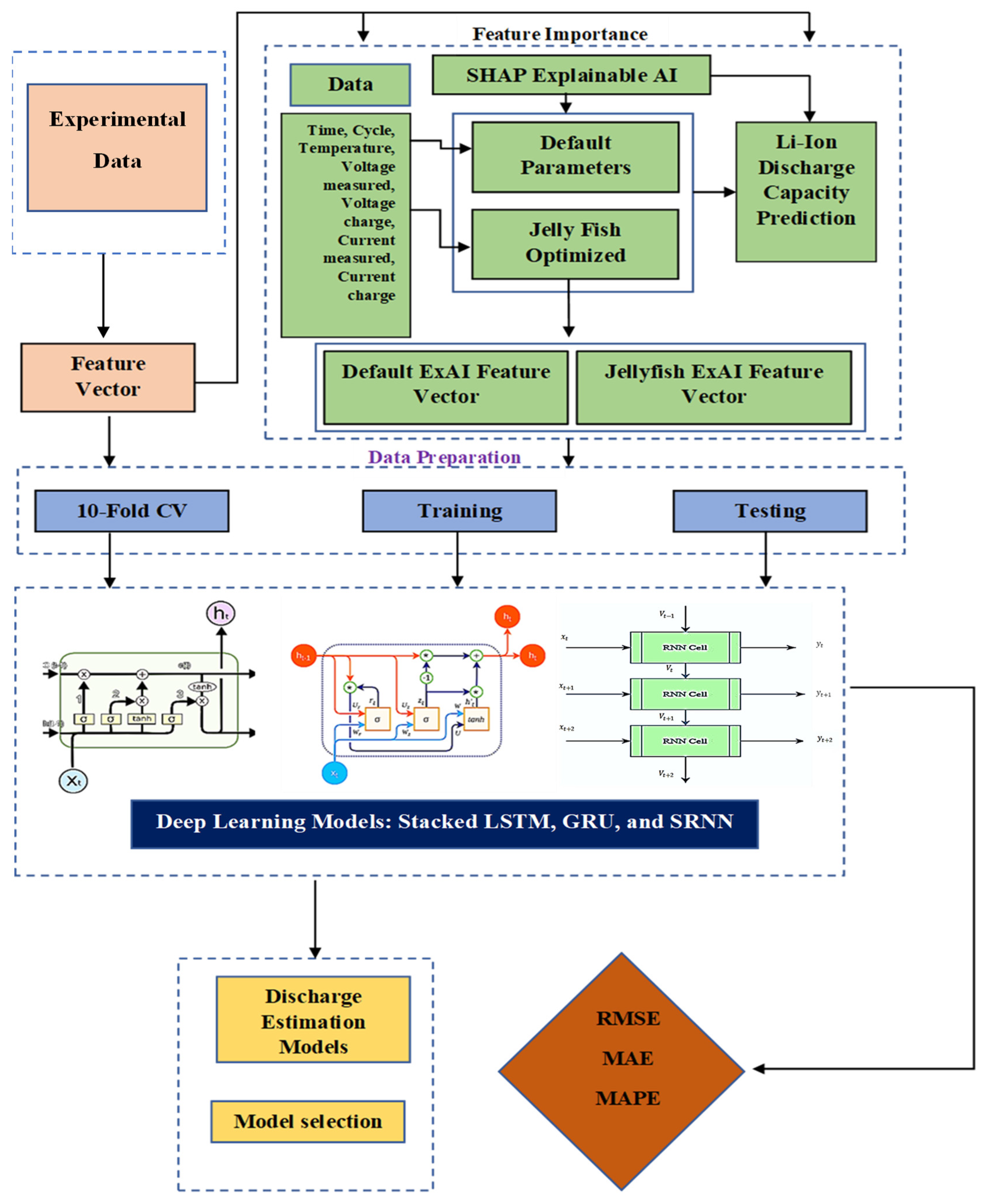
2. Materials and Methods
2.1. Deep Learning Algorithms
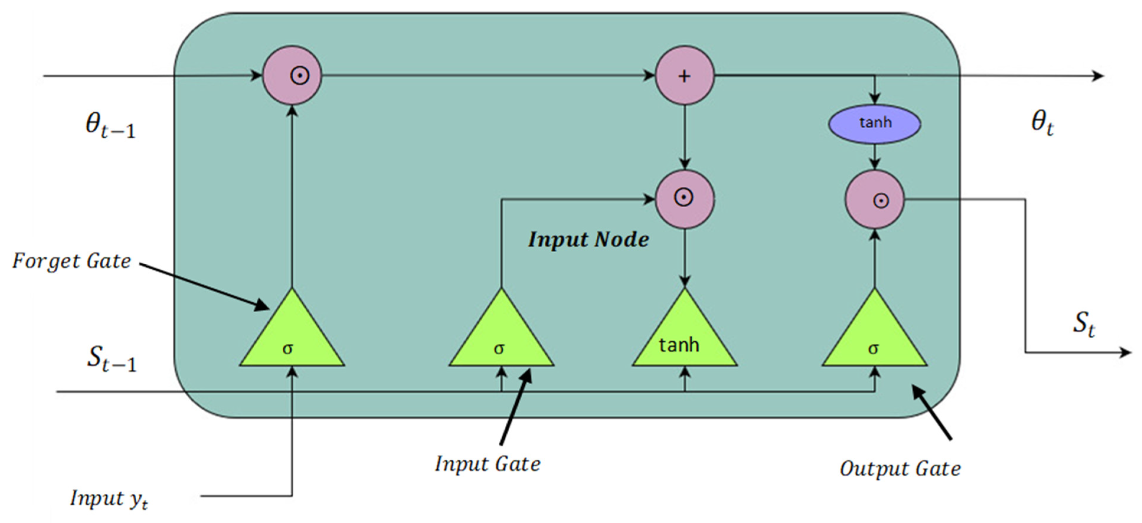
2.1.1. Stacked Long Short-Term Memory Network
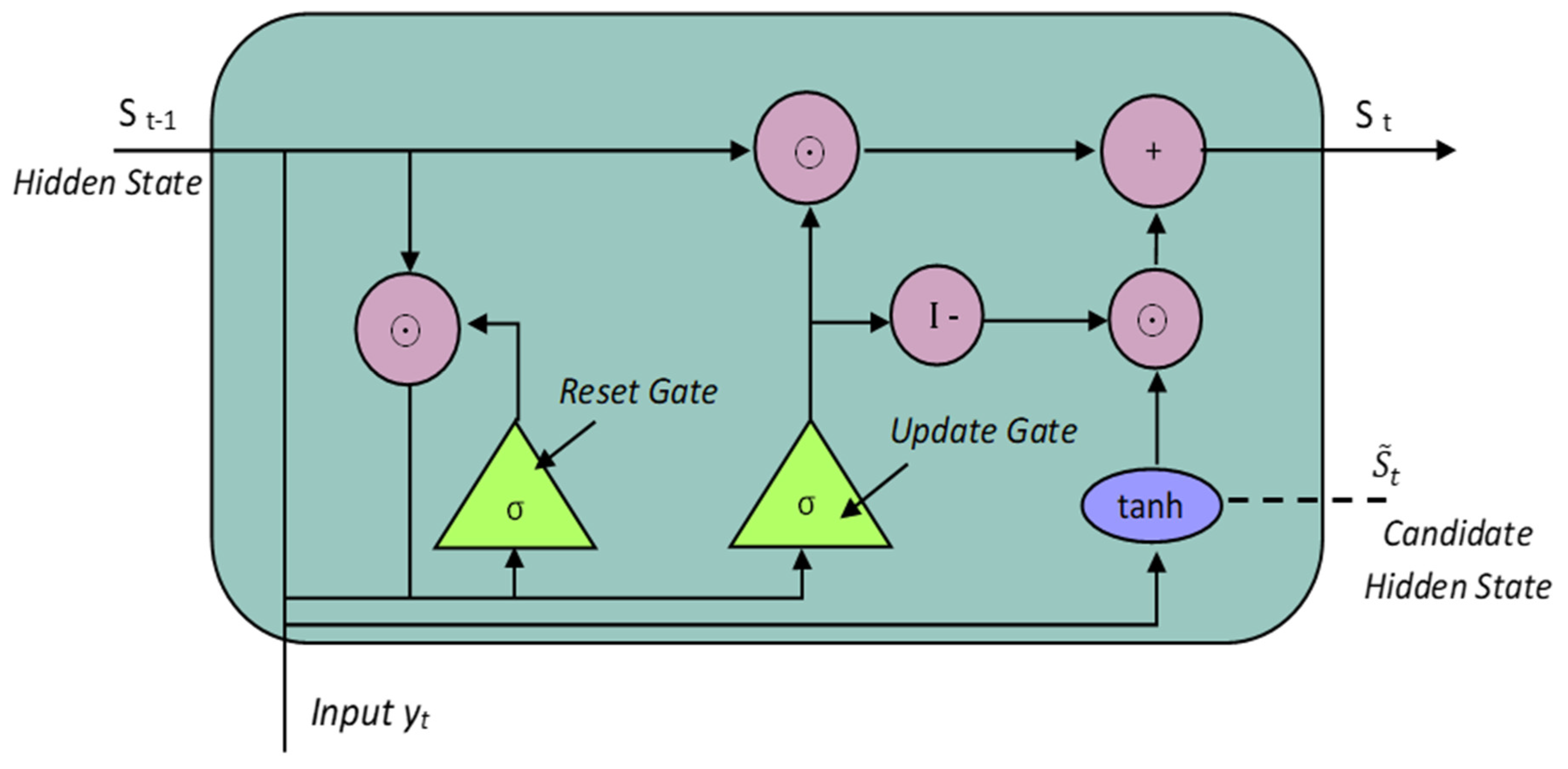
2.1.2. Gated Recurrent Unit
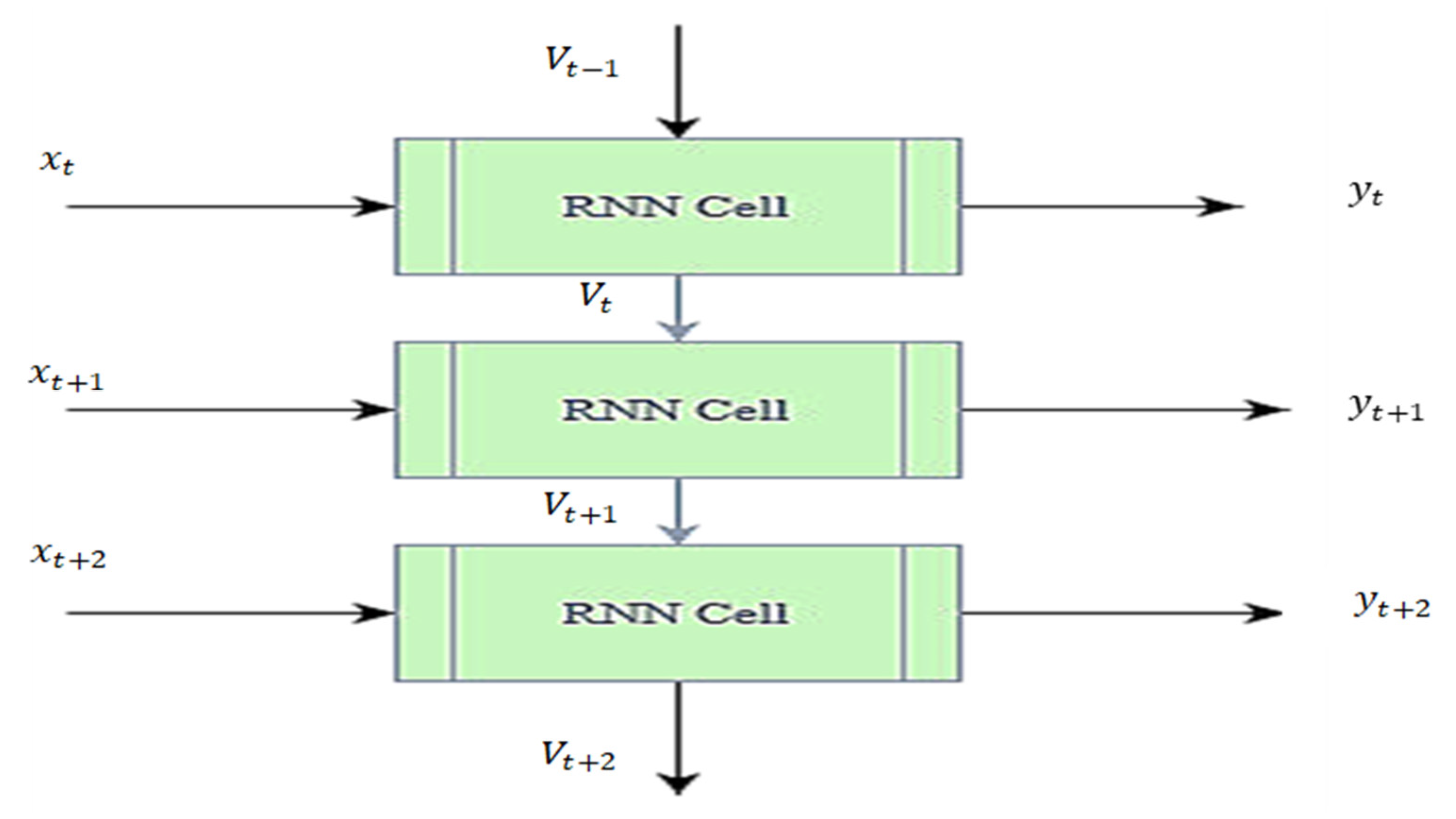
2.1.3. Stacked Recurrent Neural Network
2.2. Jellyfish Optimization
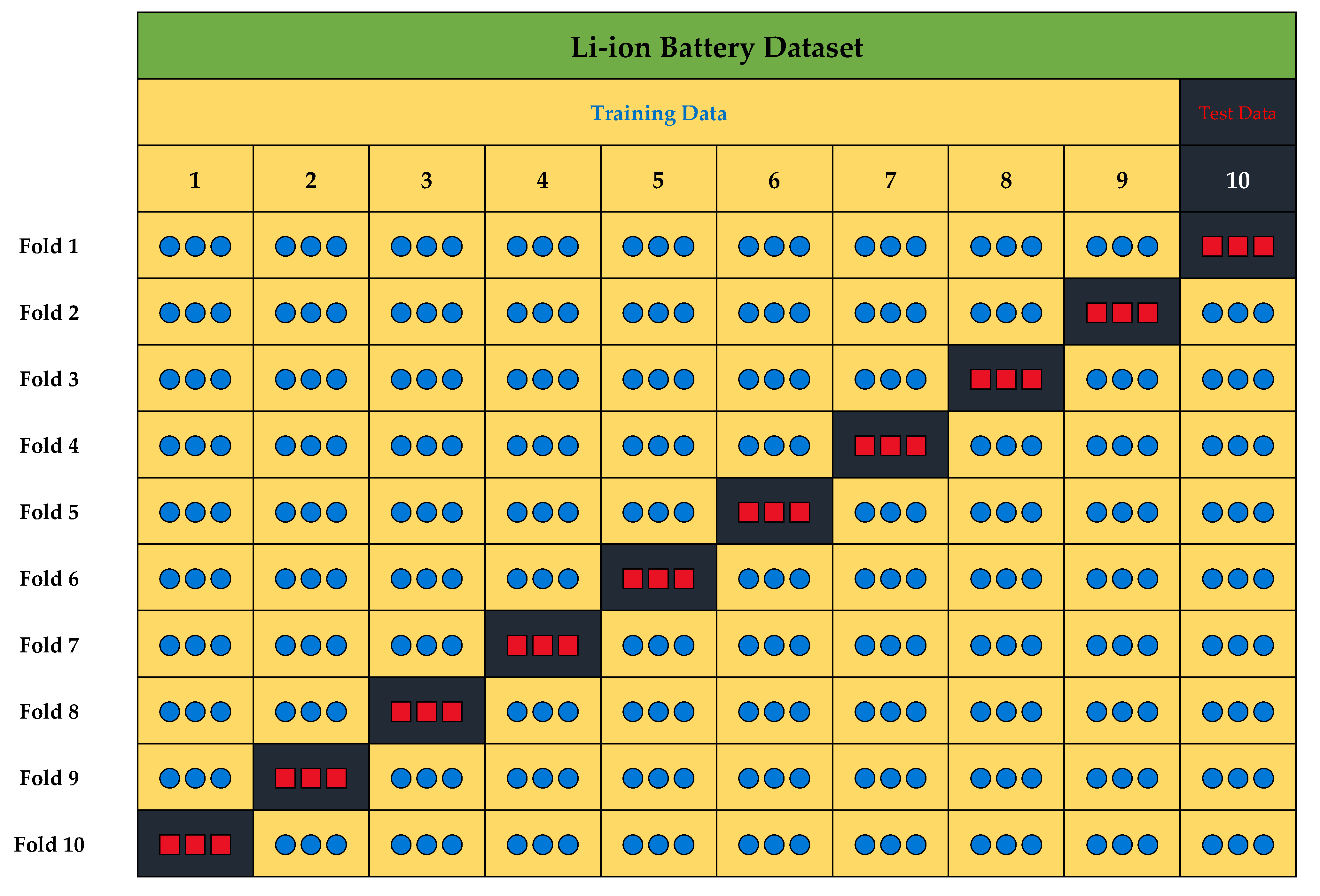
2.3. Experimentation and Data Acquisition
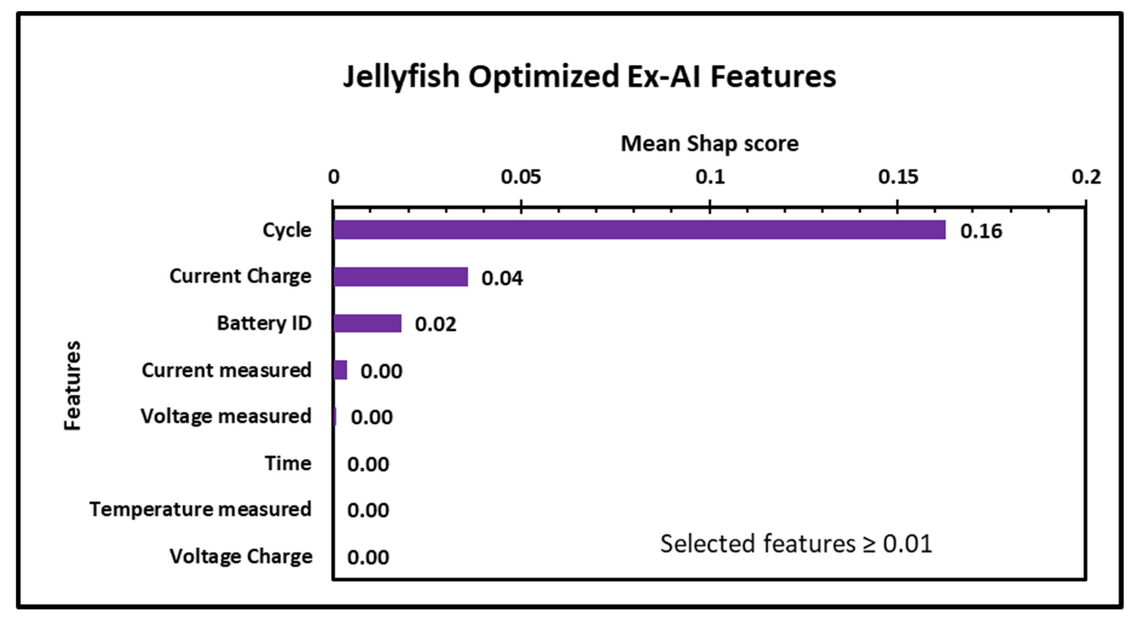
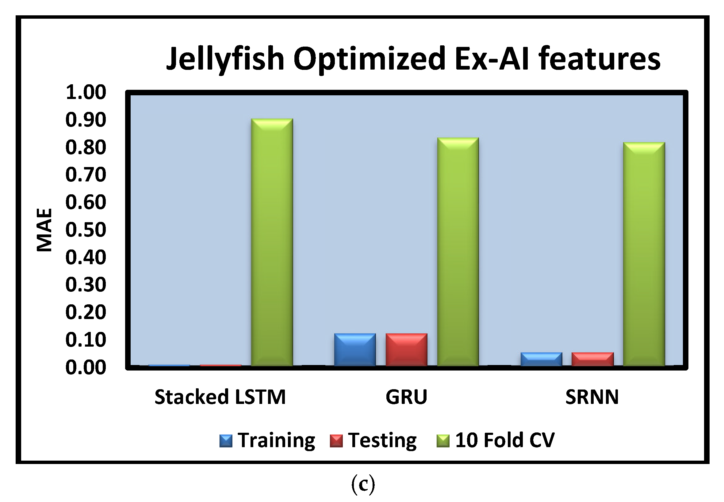
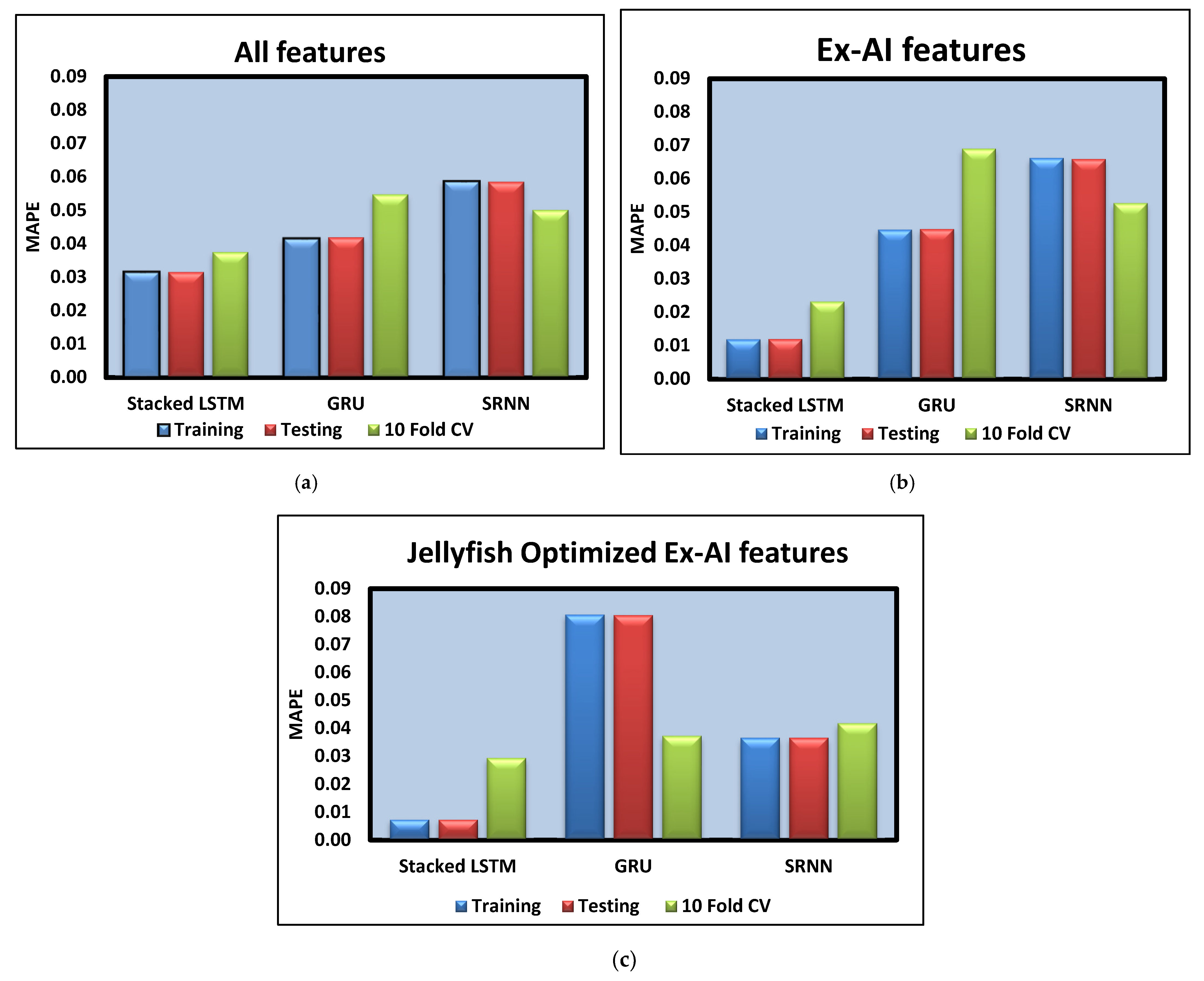
3. Results and Discussion
4. Conclusions
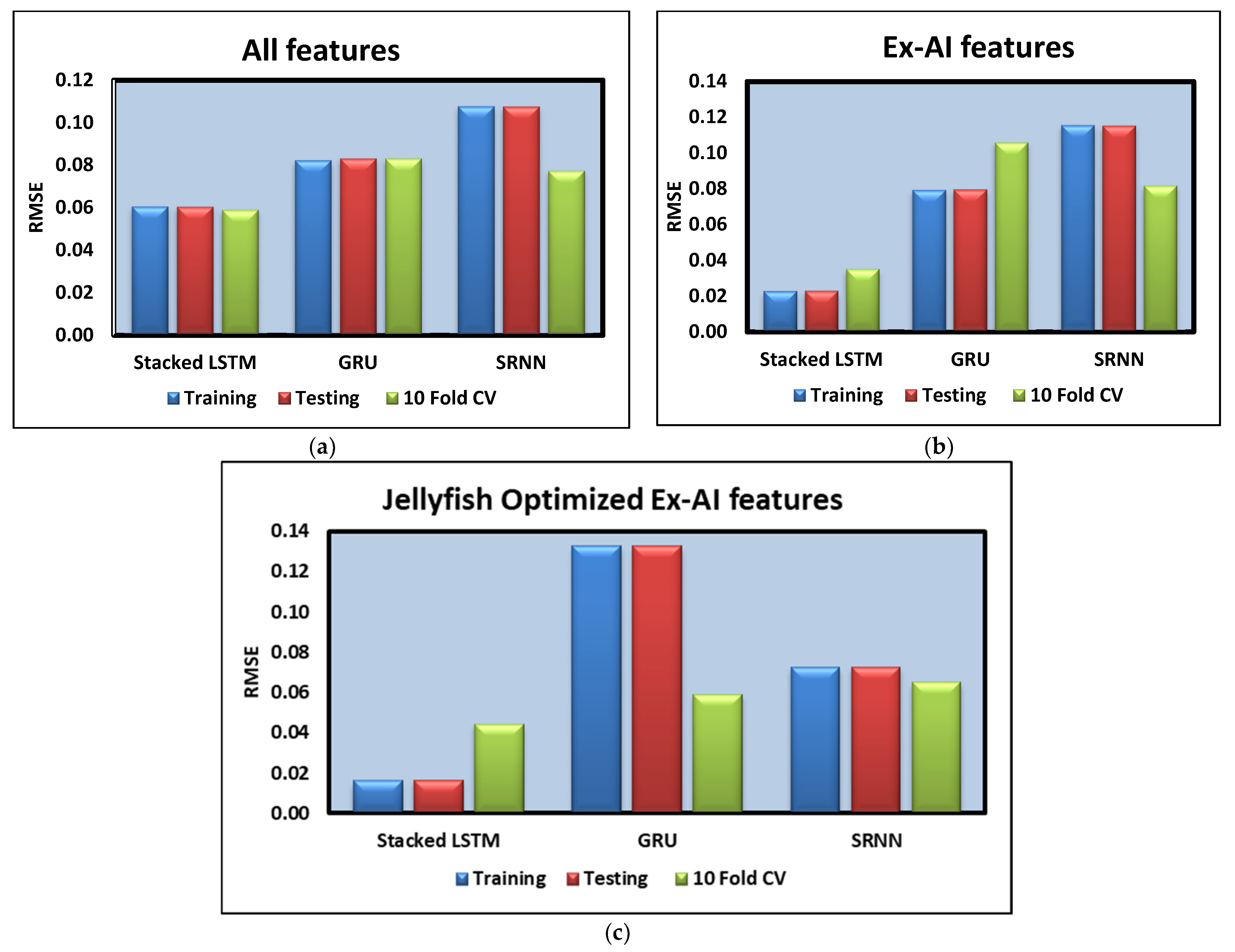
- The lowest RMSE value of 0.04 is observed from the stacked LSTM model when jellyfish-optimized Ex-AI features were considered.
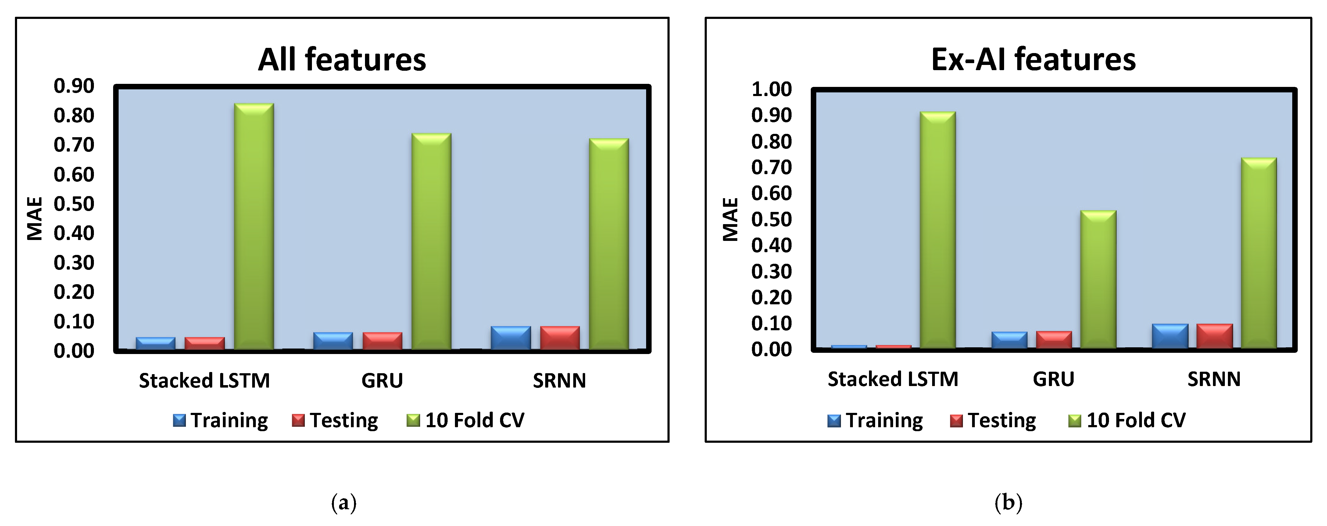
- Very low MAE and MAPE of 0.01 were obtained from the stacked LSTM model when jellyfish-optimized Ex-AI features were considered.
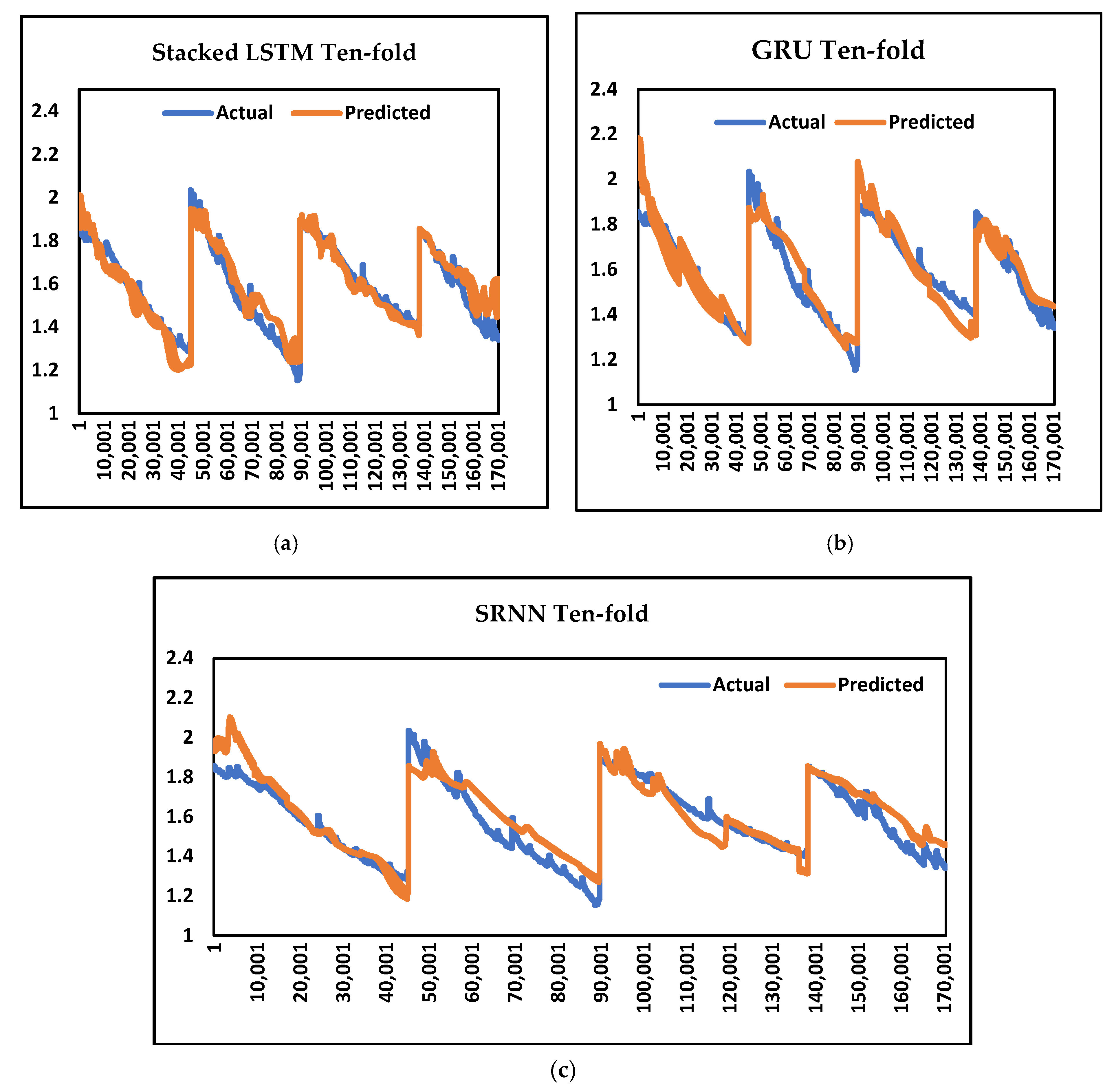
- Stacked LSTM better predicts the discharge capacity of Li-ion batteries as compared to GRU and SRNN deep learning models.
- Features selected after applying jellyfish-optimized Ex-AI models were found to exhibit better prediction capability compared to both Ex-AI features and all features.
Author Contributions
Funding
Institutional Review Board Statement
Informed Consent Statement
Data Availability Statement
Acknowledgments
Conflicts of Interest
References
- Zhang, L.; Wang, S.; Qu, X. Optimal Electric Bus Fleet Scheduling Considering Battery Degradation and Non-Linear Charging Profile. Transp. Res. Part E Logist. Transp. Rev. 2021, 154, 102445. [Google Scholar]
- Zhang, L.; Zeng, Z.; Qu, X. On The Role of Battery Capacity Fading Mechanism in The Lifecycle Cost of Electric Bus Fleet. IEEE Trans. Intell. Transp. Syst. 2021, 22, 2371–2380. [Google Scholar]
- Zhang, W.; Zhao, H.; Xu, M. Optimal Operating Strategy of Short Turning Lines for The Battery Electric Bus System. Commun. Transp. Res. 2021, 1, 100023. [Google Scholar]
- Reza, M.; Mannan, M.; Wali, S.; Hannan, M.; Jern, K.; Rahman, S.; Muttaqi, K.; Mahlia, T. Energy Storage Integration Towards Achieving Grid Decarbonization: A Bibliometric Analysis and Future Directions. J. Energy Storage 2021, 41, 102855. [Google Scholar] [CrossRef]
- Hannan, M.; Faisal, M.; Jern Ker, P.; Begum, R.; Dong, Z.; Zhang, C. Review of Optimal Methods and Algorithms for Sizing Energy Storage Systems to Achieve Decarbonization in Microgrid Applications. Renew. Sustain. Energy Rev. 2020, 131, 110022. [Google Scholar] [CrossRef]
- Wen, J.; Zhao, D.; Zhang, C. An Overview of Electricity Powered Vehicles: Lithium-Ion Battery Energy Storage Density and Energy Conversion Efficiency. Renew. Energy 2020, 162, 1629–1648. [Google Scholar]
- Wu, J.; Wang, Y.; Zhang, X.; Chen, Z. A Novel State of Health Estimation Method of Li-Ion Battery Using Group Method of Data Handling. J. Power Sources 2016, 327, 457–464. [Google Scholar] [CrossRef]
- Xiong, R.; Yu, Q.; Shen, W.; Lin, C.; Sun, F. A Sensor Fault Diagnosis Method for A Lithium-Ion Battery Pack in Electric Vehicles. IEEE Trans. Power Electron. 2019, 34, 9709–9718. [Google Scholar]
- Rivera-Barrera, J.; Muñoz-Galeano, N.; Sarmiento-Maldonado, H. Soc Estimation for Lithium-Ion Batteries: Review and Future Challenges. Electronics 2017, 6, 102. [Google Scholar] [CrossRef]
- El Mejdoubi, A.; Oukaour, A.; Chaoui, H.; Gualous, H.; Sabor, J.; Slamani, Y. State-Of-Charge and State-Of-Health Lithium-Ion Batteries’ Diagnosis According to Surface Temperature Variation. IEEE Trans. Ind. Electron. 2016, 63, 2391–2402. [Google Scholar] [CrossRef]
- Yu, J. State-Of-Health Monitoring and Prediction of Lithium-Ion Battery Using Probabilistic Indication and State-Space Model. IEEE Trans. Instrum. Meas. 2015, 64, 2937–2949. [Google Scholar]
- Pascoe, P.; Anbuky, A. Standby Power System VRLA Battery Reserve Life Estimation Scheme. IEEE Trans. Energy Convers. 2005, 20, 887–895. [Google Scholar]
- Zhi, Y.; Wang, H.; Wang, L. A State of Health Estimation Method for Electric Vehicle Li-Ion Batteries Using GA-PSO-SVR. Complex Intell. Syst. 2022, 8, 2167–2182. [Google Scholar]
- Bhavsar, K.; Vakharia, V.; Chaudhari, R.; Vora, J.; Pimenov, D.; Giasin, K. A Comparative Study to Predict Bearing Degradation Using Discrete Wavelet Transform (DWT), Tabular Generative Adversarial Networks (TGAN) and Machine Learning Models. Machines 2022, 10, 176. [Google Scholar]
- Vakharia, V.; Vora, J.; Khanna, S.; Chaudhari, R.; Shah, M.; Pimenov, D.Y.; Giasin, K.; Prajapati, P.; Wojciechowski, S. Experimental investigations and prediction of WEDMed surface of nitinol SMA using SinGAN and DenseNet deep learning model. J. Mater. Res. Technol. 2022, 18, 325–337. [Google Scholar]
- Mishra, A.; Dasgupta, A. Supervised and Unsupervised Machine Learning Algorithms for Forecasting the Fracture Location in Dissimilar Friction-Stir-Welded Joints. Forecasting 2022, 4, 787–797. [Google Scholar] [CrossRef]
- Xiong, R.; Li, L.; Tian, J. Towards A Smarter Battery Management System: A Critical Review on Battery State of Health Monitoring Methods. J. Power Sources 2018, 405, 18–29. [Google Scholar]
- Li, J.; Adewuyi, K.; Lotfi, N.; Landers, R.; Park, J. A Single Particle Model with Chemical/Mechanical Degradation Physics for Lithium-Ion Battery State of Health (SOH) Estimation. Appl. Energy 2018, 212, 1178–1190. [Google Scholar]
- Gao, Y.; Liu, K.; Zhu, C.; Zhang, X.; Zhang, D. Co-Estimation of State-of-Charge and State-of- Health for Lithium-Ion Batteries Using an Enhanced Electrochemical Model. IEEE Trans. Ind. Electron. 2022, 69, 2684–2696. [Google Scholar] [CrossRef]
- Wu, L.; Pang, H.; Geng, Y.; Liu, X.; Liu, J.; Liu, K. Low-Complexity State of Charge and Anode Potential Prediction for Lithium-Ion Batteries Using a Simplified Electrochemical Model-Based Observer under Variable Load Condition. Int. J. Energy Res. 2022, 46, 11834–11848. [Google Scholar]
- Wei, Z.; Zhao, J.; Ji, D.; Tseng, K. A Multi-Timescale Estimator for Battery State of Charge and Capacity Dual Estimation Based on An Online Identified Model. Appl. Energy 2017, 204, 1264–1274. [Google Scholar] [CrossRef]
- Yu, J.; Mo, B.; Tang, D.; Liu, H.; Wan, J. Remaining Useful Life Prediction for Lithium-Ion Batteries Using a Quantum Particle Swarm Optimization-Based Particle Filter. Qual. Eng. 2017, 29, 536–546. [Google Scholar]
- Torai, S.; Nakagomi, M.; Yoshitake, S.; Yamaguchi, S.; Oyama, N. State-Of-Health Estimation of Lifepo4/Graphite Batteries Based on a Model Using Differential Capacity. J. Power Sources 2016, 306, 62–69. [Google Scholar]
- Cui, S.; Joe, I. A Dynamic Spatial-Temporal Attention-Based GRU Model with Healthy Features for State-of-Health Estimation of Lithium-Ion Batteries. IEEE Access 2021, 9, 27374–27388. [Google Scholar]
- Patil, M.; Tagade, P.; Hariharan, K.; Kolake, S.; Song, T.; Yeo, T.; Doo, S. A Novel Multistage Support Vector Machine Based Approach for Li Ion Battery Remaining Useful Life Estimation. Appl. Energy 2015, 159, 285–297. [Google Scholar]
- Nuhic, A.; Terzimehic, T.; Soczka-Guth, T.; Buchholz, M.; Dietmayer, K. Health Diagnosis and Remaining Useful Life Prognostics of Lithium-Ion Batteries Using Data-Driven Methods. J. Power Sources 2013, 239, 680–688. [Google Scholar] [CrossRef]
- Zheng, X.; Deng, X. State-of-Health Prediction for Lithium-Ion Batteries with Multiple Gaussian Process Regression Model. IEEE Access 2019, 7, 150383–150394. [Google Scholar]
- Sun, B.; Pan, J.; Wu, Z.; Xia, Q.; Wang, Z.; Ren, Y.; Yang, D.; Guo, X.; Feng, Q. Adaptive evolution enhanced physics-informed neural networks for time-variant health prognosis of lithium-ion batteries. J. Power Sources 2023, 556, 232432. [Google Scholar] [CrossRef]
- Patel, D.R.; Kiran, M.B.; Vakharia, V. Modeling and prediction of surface roughness using multiple regressions: A noncontact approach. Eng. Rep. 2020, 2, e12119. [Google Scholar] [CrossRef]
- Vakharia, V.; Kiran, M.B.; Dave, N.J.; Kagathara, U. Feature extraction and classification of machined component texture images using wavelet and artificial intelligence techniques. In Proceedings of the 2017 8th International Conference on Mechanical and Aerospace Engineering (ICMAE), Prague, Czech Republic, 22–25 July 2017; pp. 140–144. [Google Scholar] [CrossRef]
- Shah, M.; Vakharia, V.; Chaudhari, R.; Vora, J.; Pimenov, D.; Giasin, K. Tool Wear Prediction in Face Milling of Stainless Steel Using Singular Generative Adversarial Network And LSTM Deep Learning Models. Int. J. Adv. Manuf. Technol. 2022, 121, 723–736. [Google Scholar] [CrossRef]
- Pang, H.; Wu, L.; Liu, J.; Liu, X.; Liu, K. Physics-informed neural network approach for heat generation rate estimation of lithium-ion battery under various driving conditions. J. Energy Chem. 2023, 78, 1–12. [Google Scholar] [CrossRef]
- Cho, K.; Van Merriënboer, B.; Gulcehre, C.; Bahdanau, D.; Bougares, F.; Schwenk, H.; Bengio, Y. Learning phrase representations using RNN encoder-decoder for statistical machine translation. arXiv 2014, arXiv:1406.1078. [Google Scholar]
- Čerňanský, M.; Makula, M.; Beňušková, Ľ. Organization of the state space of a simple recurrent network before and after training on recursive linguistic structures. Neural Netw. 2007, 20, 236–244. [Google Scholar] [CrossRef] [PubMed]
- Liu, X.; Zhou, J.; Qian, H. Short-Term Wind Power Forecasting by Stacked Recurrent Neural Networks with Parametric Sine Activation Function. Electr. Power Syst. Res. 2021, 192, 107011. [Google Scholar] [CrossRef]
- Chou, J.; Truong, D. A Novel Metaheuristic Optimizer Inspired by Behavior of Jellyfish in Ocean. Appl. Math. Comput. 2021, 389, 125535. [Google Scholar] [CrossRef]
- Saha, B.; Goebel, K. Battery Data Set. In NASA Ames Prognostics Data Repository; NASA Ames Research Centre: Mountain View, CA, USA, 2007. Available online: https://ti.arc.nasa.gov/tech/dash/groups/pcoe/prognosticdata-repository/ (accessed on 1 September 2022).


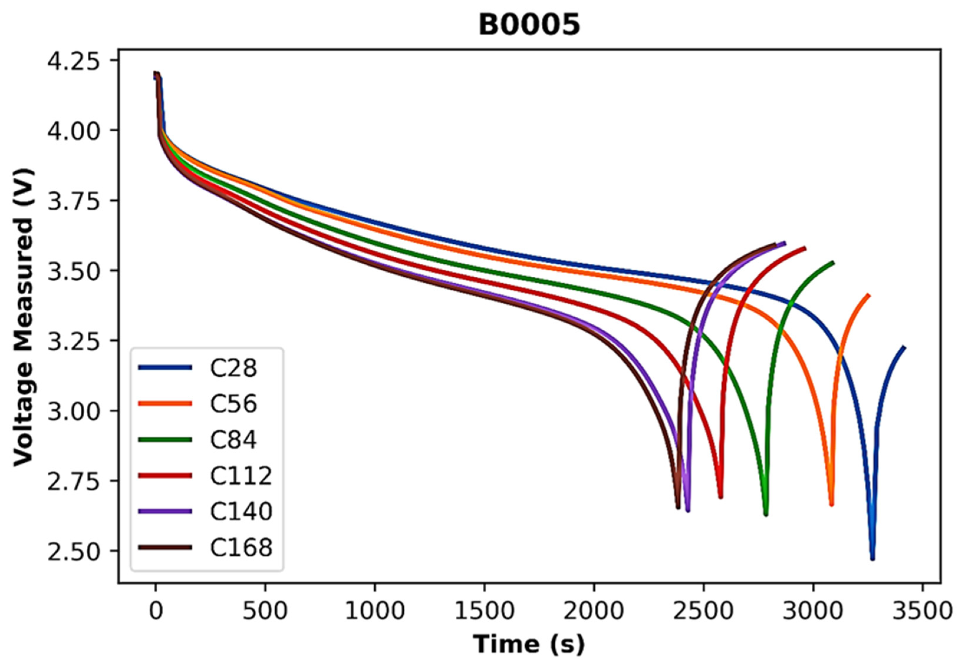
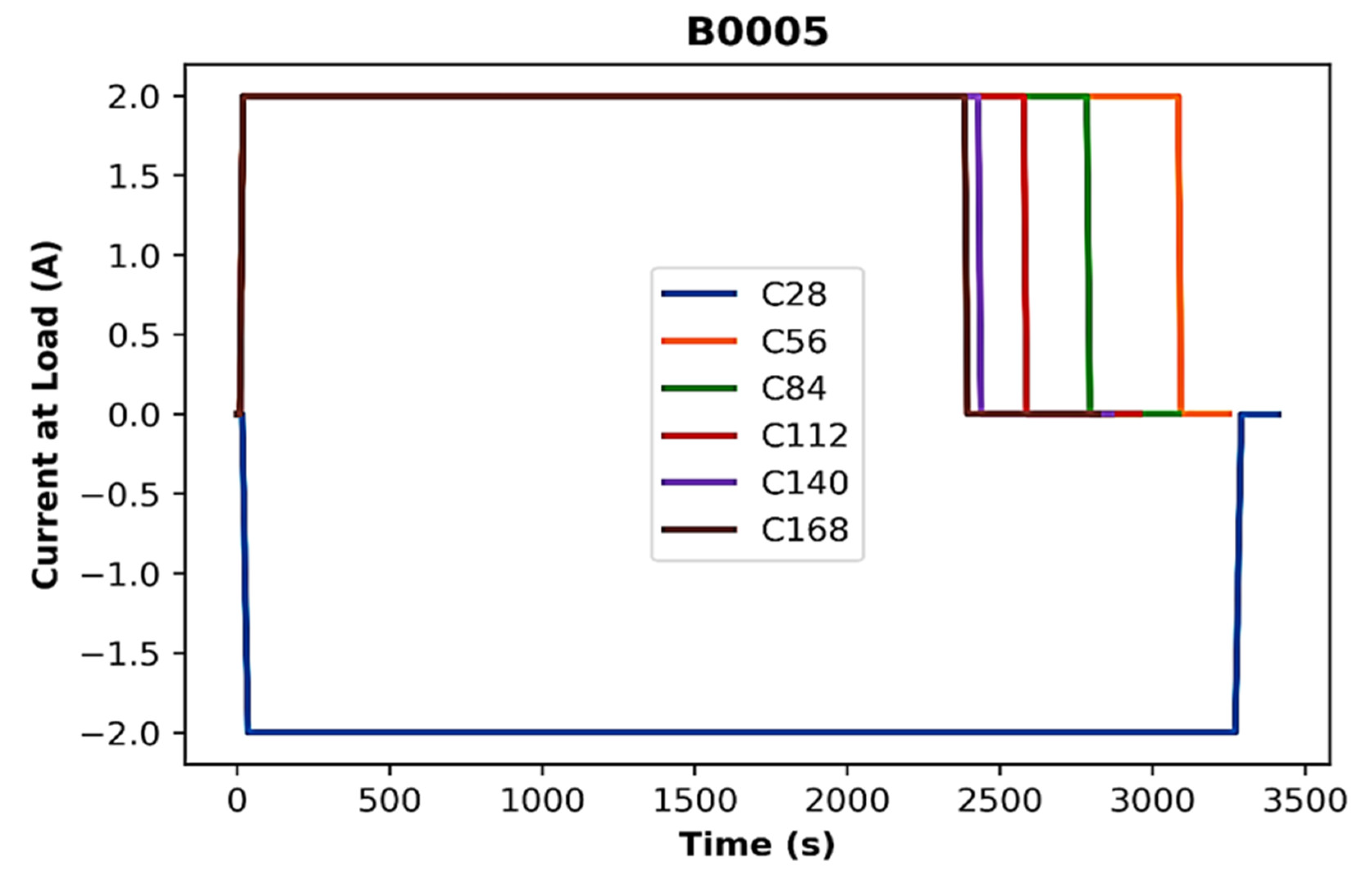
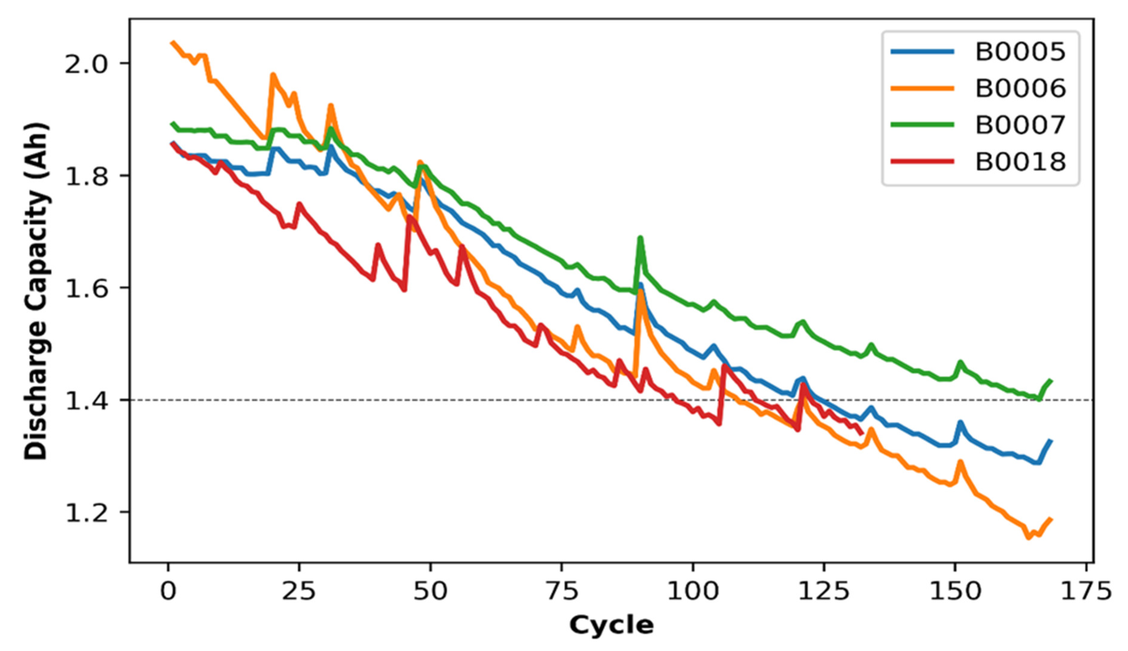
| Battery No. | Ambient Temperature | No. of Cycles | Discharge Cut-Off Voltage |
|---|---|---|---|
| B0005 | 24 °C | 168 | 2.7 V |
| B0006 | 24 °C | 168 | 2.5 V |
| B0007 | 24 °C | 168 | 2.2 V |
| B0018 | 24 °C | 132 | 2.5 V |
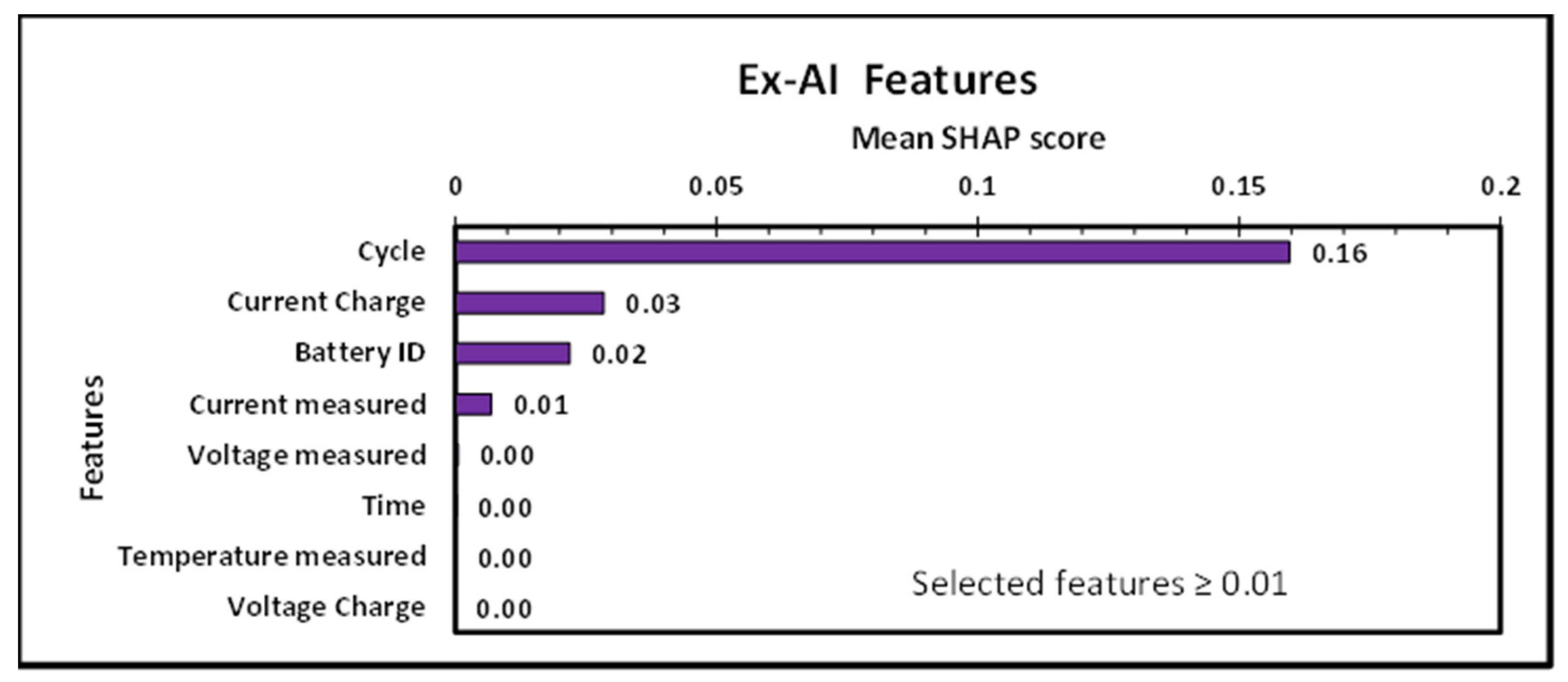
| Feature Name | Description |
|---|---|
| Voltage measured | Battery terminal voltage during discharge (Volts) |
| Current measured | Battery output during discharge (Amp) |
| Temperature measured | Battery temperature measured during discharge (°C) |
| Current charge | Current measured at the load during discharge (Amp) |
| Voltage charge | Voltage measured at the load during discharge (Volts) |
| Time | Time vector from start to end of a discharge cycle (secs) |
| Cycle | Number of discharge cycles for battery |
| Battery ID | To identify the battery number among four batteries |
| XGBoost Parameters | Function | Range |
|---|---|---|
| P1 | Learning rate | (0,1] |
| P2 | Max depth | [0,inf) |
| P3 | Min child weight | [0,inf) |
| P4 | N estimators | [50,500] |
| P5 | N jobs | [1,inf) |
| P6 | Subsamples | (0,1] |
| XGBoost | P1 | P2 | P3 | P4 | P5 | P6 |
|---|---|---|---|---|---|---|
| Default | 0.3 | 6 | 1 | 100 | 1 | 1 |
| Jellyfish | 0.10 | 2 | 2.79 | 307 | 1 | 0.98 |
| Feature | Model | Stacked LSTM | GRU | SRNN | ||||||
|---|---|---|---|---|---|---|---|---|---|---|
| Metrics | Train | Test | Ten-Fold | Train | Test | Ten-Fold | Train | Test | Ten-Fold | |
| Voltage measured | RMSE | 0.187 | 0.187 | 0.194 | 0.186 | 0.187 | 0.209 | 0.229 | 0.229 | 0.227 |
| MAE | 0.360 | 0.362 | 1.336 | 0.358 | 0.358 | 1.424 | 0.412 | 0.414 | 1.512 | |
| MAPE | 0.104 | 0.104 | 0.118 | 0.103 | 0.103 | 0.111 | 0.110 | 0.110 | 0.115 | |
| Current measured | RMSE | 0.190 | 0.191 | 0.196 | 0.206 | 0.207 | 0.212 | 0.190 | 0.190 | 0.208 |
| MAE | 0.365 | 0.367 | 1.360 | 0.396 | 0.396 | 1.480 | 0.365 | 0.367 | 1.416 | |
| MAPE | 0.103 | 0.104 | 0.119 | 0.118 | 0.118 | 0.122 | 0.104 | 0.104 | 0.112 | |
| Temperature measured | RMSE | 0.190 | 0.190 | 0.194 | 0.259 | 0.260 | 0.242 | 0.195 | 0.196 | 0.208 |
| MAE | 0.367 | 0.369 | 1.344 | 0.479 | 0.482 | 1.664 | 0.369 | 0.371 | 1.472 | |
| MAPE | 0.106 | 0.106 | 0.120 | 0.147 | 0.148 | 0.132 | 0.103 | 0.103 | 0.128 | |
| Current charge | RMSE | 0.164 | 0.165 | 0.173 | 0.180 | 0.181 | 0.176 | 0.179 | 0.180 | 0.186 |
| MAE | 0.308 | 0.311 | 1.168 | 0.324 | 0.329 | 1.192 | 0.335 | 0.338 | 1.272 | |
| MAPE | 0.102 | 0.101 | 0.115 | 0.100 | 0.100 | 0.107 | 0.101 | 0.101 | 0.159 | |
| Voltage charged | RMSE | 0.183 | 0.184 | 0.192 | 0.186 | 0.187 | 0.205 | 0.191 | 0.191 | 0.223 |
| MAE | 0.351 | 0.353 | 1.320 | 0.356 | 0.356 | 1.384 | 0.358 | 0.360 | 1.488 | |
| MAPE | 0.156 | 0.157 | 0.165 | 0.158 | 0.158 | 0.173 | 0.159 | 0.160 | 0.186 | |
| Time | RMSE | 0.189 | 0.190 | 0.196 | 0.378 | 0.378 | 0.228 | 0.222 | 0.223 | 0.208 |
| MAE | 0.365 | 0.367 | 1.360 | 0.743 | 0.743 | 1.560 | 0.405 | 0.407 | 1.480 | |
| MAPE | 0.104 | 0.104 | 0.119 | 0.197 | 0.198 | 0.123 | 0.109 | 0.109 | 0.118 | |
| Cycle | RMSE | 0.100 | 0.102 | 0.195 | 0.117 | 0.117 | 0.133 | 0.103 | 0.104 | 0.105 |
| MAE | 0.285 | 0.290 | 1.027 | 0.475 | 0.475 | 1.521 | 0.430 | 0.435 | 1.092 | |
| MAPE | 0.107 | 0.107 | 0.151 | 0.104 | 0.104 | 0.176 | 0.103 | 0.104 | 0.155 | |
| LSTM | GRU | SRNN | ||
|---|---|---|---|---|
| Features | Validation | Time (s) | Time (s) | Time (s) |
| All features | Train | 330 | 270 | 550 |
| Test | 30 | 11 | 13 | |
| 10 CV | 4200 | 3500 | 6500 | |
| Ex-AI features | Train | 308 | 230 | 510 |
| Test | 30 | 10 | 10 | |
| 10 CV | 3900 | 3300 | 6200 | |
| Optimized Ex-AI Features | Train | 300 | 220 | 490 |
| Test | 27 | 10 | 10 | |
| 10 CV | 3500 | 3200 | 6000 |
Disclaimer/Publisher’s Note: The statements, opinions and data contained in all publications are solely those of the individual author(s) and contributor(s) and not of MDPI and/or the editor(s). MDPI and/or the editor(s) disclaim responsibility for any injury to people or property resulting from any ideas, methods, instructions or products referred to in the content. |
© 2023 by the authors. Licensee MDPI, Basel, Switzerland. This article is an open access article distributed under the terms and conditions of the Creative Commons Attribution (CC BY) license (https://creativecommons.org/licenses/by/4.0/).
Share and Cite
Vakharia, V.; Shah, M.; Nair, P.; Borade, H.; Sahlot, P.; Wankhede, V. Estimation of Lithium-ion Battery Discharge Capacity by Integrating Optimized Explainable-AI and Stacked LSTM Model. Batteries 2023, 9, 125. https://doi.org/10.3390/batteries9020125
Vakharia V, Shah M, Nair P, Borade H, Sahlot P, Wankhede V. Estimation of Lithium-ion Battery Discharge Capacity by Integrating Optimized Explainable-AI and Stacked LSTM Model. Batteries. 2023; 9(2):125. https://doi.org/10.3390/batteries9020125
Chicago/Turabian StyleVakharia, Vinay, Milind Shah, Pranav Nair, Himanshu Borade, Pankaj Sahlot, and Vishal Wankhede. 2023. "Estimation of Lithium-ion Battery Discharge Capacity by Integrating Optimized Explainable-AI and Stacked LSTM Model" Batteries 9, no. 2: 125. https://doi.org/10.3390/batteries9020125
APA StyleVakharia, V., Shah, M., Nair, P., Borade, H., Sahlot, P., & Wankhede, V. (2023). Estimation of Lithium-ion Battery Discharge Capacity by Integrating Optimized Explainable-AI and Stacked LSTM Model. Batteries, 9(2), 125. https://doi.org/10.3390/batteries9020125