Article

Hybrid Estimation Method for the State of Charge of Lithium Batteries Using a Temporal Convolutional Network and XGBoost

School of Electronic and Electrical Engineering, Kyungpook National University, Daegu 41566, Republic of Korea
*
Author to whom correspondence should be addressed.
Batteries 2023, 9(11), 544; https://doi.org/10.3390/batteries9110544
Submission received: 28 September 2023 / Revised: 21 October 2023 / Accepted: 3 November 2023 / Published: 5 November 2023
(This article belongs to the Special Issue Recent Advances in Battery Measurement and Management Systems)

Abstract

:
Lithium batteries have recently attracted significant attention as highly promising energy storage devices within the secondary battery industry. However, it is important to note that they may pose safety risks, including the potential for explosions during use. Therefore, achieving stable and safe utilization of these batteries necessitates accurate state-of-charge (SOC) estimation. In this study, we propose a hybrid model combining temporal convolutional network (TCN) and eXtreme gradient boosting (XGBoost) to investigate the nonlinear and evolving characteristics of batteries. The primary goal is to enhance SOC estimation performance by leveraging TCN’s long-effective memory capabilities and XGBoost’s robust generalization abilities. We conducted experiments using datasets from NASA, Oxford, and a vehicle simulator to validate the model’s performance. Additionally, we compared the performance of our model with that of a multilayer neural network, long short-term memory, gated recurrent unit, XGBoost, and TCN. The experimental results confirm that our proposed TCN–XGBoost hybrid model outperforms the other models in SOC estimation across all datasets.

1. Introduction

Lithium batteries have recently attracted considerable attention as the most promising energy storage devices in the secondary battery industry because of their high energy density, long service life, low memory effect, and low self-discharge rate [1,2]. Lithium-ion batteries are widely employed in various fields, including mobile devices, electric vehicles, and energy storage systems. However, these batteries have potential safety risks. In particular, concerns arise owing to their potential to harm human life and damage properties in cases where these batteries explode during usage. The safety problems associated with lithium-ion batteries can be attributed to various factors, with the primary causes being the following [3,4]: (1) battery explosions resulting from overheating; (2) battery explosions caused by overcharging and overdischarging; and (3) battery explosions due to physical damage. Herein, we propose a model for accurately estimating the state of charge (SOC) of batteries to proactively prevent battery explosions caused by overcharging and overdischarging [5,6,7,8]. The state of charge (SOC) of a battery is not a directly measurable parameter; it is defined as the percentage of available capacity remaining in relation to the nominal capacity. Therefore, SOC must be indirectly estimated using an SOC estimation algorithm based on battery parameters obtained from sensor measurements. However, accurately estimating the battery SOC is challenging due to the nonlinear nature of lithium battery parameters and their susceptibility to change based on the operating environment [9,10].
In recent times, numerous researchers have been engaged in exploring SOC estimation methods. These methods can be broadly categorized into three main types: model-based, data-driven, and coulomb counting methods [11]. Model-based methods are known for their robustness and high accuracy, primarily because they are built upon a comprehensive understanding of the system. However, they can face practical and theoretical challenges in creating a flawless model for the target system. On the other hand, data-driven methods do not necessitate practitioners to possess in-depth, specific knowledge of the target system since they rely on data analysis. Nevertheless, they do demand a substantial volume of data for reliable performance. Coulomb counting methods entail measuring a battery’s discharge current and integrating it over time to estimate the current capacity of the battery. In Table 1, we present a summary outlining the advancements and limitations of these three methodological approaches.
In the table, the equivalent circuit model provides an abstract representation of a lithium battery by combining parameters such as resistance, capacitance, and inductance. However, due to its reliance on electrical characteristics, this model falls short of fully elucidating the battery’s internal reactions [24]. In the case of the open-circuit voltage (OCV)–SOC model, SOC estimation relies on modeling SOC based on the battery’s OCV. While this approach is known for its ease of implementation and accuracy, it remains susceptible to uncertainties stemming from factors such as temperature, aging, and driving cycles [25]. In the Coulomb counting model, battery current capacity is estimated using a cumulative current integration method. Although this approach is straightforward to implement, prolonged use may result in the accumulation of measurement errors, leading to a subsequent decrease in accuracy [26]. Within the context of the Kalman filter, it becomes possible to learn and estimate the nonlinear characteristics of a battery in real-time. However, as the predicted state variable increases, computational complexity grows, which in turn extends the calculation times [27]. In the case of neural networks and deep learning models, they acquire knowledge of the relationship between a battery’s capacity and its parameters by analyzing measurements taken directly from the battery. The primary challenge encountered by these models is the accurate capture of the battery’s aging process through the extraction of valuable features from the measured signals [28].
This paper proposes a hybrid estimation method using a temporal convolutional network (TCN) and eXtreme gradient boosting (XGBoost). TCNs and XGBoost are formidable algorithms in the domains of time-series data processing and prediction, respectively, with TCNs excelling at capturing temporal dependencies and XGBoost known for its ability to enhance prediction accuracy. By combining these two algorithms, this study aims to maximize the use of the time-series characteristics of battery data while improving the accuracy of the prediction model. TCNs are primarily employed for extracting temporal patterns, whereas XGBoost serves as a high-performance prediction model. TCNs efficiently extract essential time-series features from input data and, by transmitting these features to the XGBoost model, allow for the separation of feature extraction and prediction. This separation facilitates model interpretability and adjustment. The main contributions of this study are as follows:
  • In the TCN part, the long-effective memory feature enables the learning of sequential battery parameters. Additionally, it facilitates the extraction of battery parameter features, enabling the model to learn the changing characteristics of batteries.
  • An information layer is employed to interface the TCN part with the XGBoost part. The information layer determines how much past information from the output of the TCN part to incorporate and transforms the output values into a one-dimensional (1D) sequence data format.
  • The output of the information layer is used as the input of XGBoost. XGBoost involves learning using a boosting algorithm, and it contributes to reducing errors in the SOC estimated through a strong generalization model. This is confirmed through the experimental results.
The remainder of the paper is organized as follows: Section 2 describes the proposed TCN-XGBoost hybrid model. Section 3 presents the analysis of the experimental results using battery data from NASA, Oxford, and vehicle simulator datasets. Section 4 provides the conclusions.

2. Proposed Lithium Battery SOC Estimation Algorithm Using the TCN-XGBoost Hybrid Model

2.1. TCN

TCN is a neural network architecture designed for processing time-series data. TCN offers notable advantages, particularly when dealing with sequence data that present challenges to traditional architectures, such as recurrent neural networks. The key characteristics of TCN can be summarized as follows [29,30]. First, TCN employs causal convolution, which ensures that information from the future is not leaked into the past. This design choice is crucial for time-series data, as it restricts the model to using only past time steps for predictions. In addition, TCN leverages dilated convolutions, allowing it to capture information from a wide range of input positions effectively. This enables the model to learn long-term dependencies and detect extended patterns within sequence data. Finally, TCN is known for its efficiency, offering a lighter model compared to architectures like WaveNet. Achieving this efficiency involves the removal of some connections and gate activations.
The TCN receives the input ( x 0 , …, x t ) and predicts the output ( y 0 , …, y t ) corresponding to each time. The key constraint is that to predict the output y t for some time t , only the present and past inputs are used.
The sequence modeling network is shown through the following equation:
y ^ 0 , . . . , y ^ t = f ( x 0   , . . . , x t   ) .
The TCN operates based on two key principles: (1) the network generates outputs of the same length as the input, and (2) it maintains a causal characteristic that prevents information leakage from the future to the past. In practical terms, this means that during the convolution operation, the output at time step t is convolved with elements from both time step t and the previous time step.
In order to meet the first characteristic, the TCN utilizes a 1D fully convolutional network (FCN), where the output hidden layer matches the length of the input hidden layer. To achieve this consistency, zero padding is applied using the kernel size −1 to retain the same length as the preceding layer. To satisfy the second causal characteristic, the TCN uses a causal convolution operation in which the convolution operation at the time t only comprises the time t of the previous layer and the time points before it. In other words, TCN = 1D FCN + causal convolutions.
The basic design of the TCN, comprising only FCN and causal conventions, has the disadvantage of using a very deep network or a large filter size to obtain a long-effective history in a long sequence. A dilated convolution is added to solve this problem.
Dilated convolution refers to a method of minimizing the amount of computation while increasing the receptive field. In simple convolution, deep layers are limited in creating large receptive fields, making it difficult to deal with sequence data affected in the distant past. On the contrary, dilated convolution makes it possible to increase exponentially according to the depth of the layer. More formally, for a 1D sequence input x R n and a filter f : { 0 , ,   k 1 } R , dilated convolution is defined as follows:
F s = x d f s = i = 0 k 1 f ( i ) · x s d · i ,
where s is the sequence, d is the dilation factor, and k is the filter size. In the context of convolution, sdi indicates shifting the filter by sdi units for each element s of the input sequence. This effectively indicates that dilation is akin to inserting a fixed length between adjacent filter elements. When d = 1, it corresponds to standard convolution, while increasing d allows for representing a considerably broader range of the input. The receptive field of the TCN can be extended by increasing the filter size k and the dilation factor d or by extending the network depth. In the TCN, the dilation factor d exponentially increases with the layer depth. This is illustrated in Figure 1.
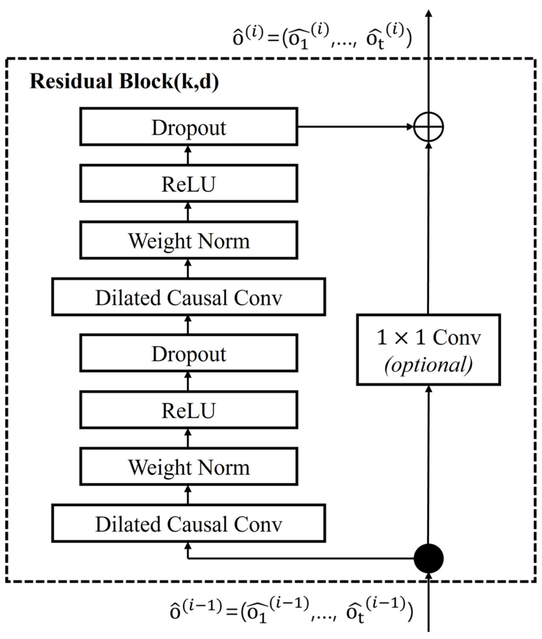
A residual connection is applied to every layer for stable training of the deep layers of the TCN. Figure 2 presents the residual block. The residual block includes dilated convolution layers with the same dilation factor d , ReLU, and dropout. At this time, the channel width of the input and the output may be different, so 1 × 1 convolution is applied to the input to match the channel width. The output of the residual block is shown in the following equation:
o = A c t i v a t i o n ( x + F x ) .

2.2. XGBoost

XGBoost is a decision tree-based ensemble machine learning algorithm that uses the gradient boosting framework. Gradient boosting is a supervised learning algorithm that uses a gradient to sequentially fit new models that compensate for the weaknesses of previous models and then linearly combine them to generate models. However, gradient boosting can cause overfitting when there is noise. XGBoost adds the parameters γ and λ to prevent the overfitting problem of gradient boosting [31,32].
XGBoost uses advanced regularization to improve its model generalization capability. Herein, the characteristics of XGBoost were combined with the TCN output.
XGBoost uses a classification and regression tree (CART) model. CART represents one value, where each node represents each dataset. The XGBoost algorithm is as follows. First, the initial model is set as a constant, as shown in the following equation:
y ^ i = ϕ o i = k = 1 K f k ( o i ) ,     f k F ,
where F is the space of the regression trees, K is the number of CARTs, y i is the predicted value of o i , and o i is the output of the TCN layer. The objective function for training each CART model is shown in the following equation:
o b j θ = i n l ( y i , y ^ i ) + k = 1 K Ω ( f k ) ,
where the left term represents the training loss, which is the difference between the actual and predicted values, while the right term serves as a regularization term to control the complexity of the tree model and prevent overfitting. l ( y i , y ^ i ) is the objective function calculated from the target value y i and the predicted value y ^ i , and Ω is the normalization function of the model to prevent overfitting. The parameters to be learned are the structure of each tree and the scores of the leaf nodes, represented as θ = f 1 , f 2 ,…, f k .
In Equation (5), f contains the structure of the tree and the predicted value of the node. It is impossible to train all the trees at once. XGBoost adds a model that predicts unexpected parts in all steps at each step. The new objective function (e.g., at step t) takes the form of an expansion represented by Taylor’s theorem, generally including up to the second order, as follows:
o b j ( t ) = i = 1 n g i f t o i + 1 2 h i f t 2 o i + Ω ( f t ) ,
where g i and h i are the primary and secondary partial differential values, respectively. The model complexity of XGBoost is shown in the following equation:
o b j ( t ) = i = 1 n Ω f = γ T + 1 2 λ j = 1 T ω 2 j ,
where ω represents a vector for node scores and T represents the number of nodes. γ T represents the number of leaves, adjusting the complexity of the model in relation to its accuracy. 1 2 λ j = 1 T ω 2 j is the L2 norm function of the leaf scores.

2.3. Proposed TCN-XGBoost Hybrid Model

The SOC of lithium batteries changes under the influence of their characteristics, degradation, and operating environment. To improve the SOC estimation accuracy, considering internal and external factors, the estimation model must model the important characteristics of the battery parameters. Therefore, we designed a TCN-XGBoost hybrid model.
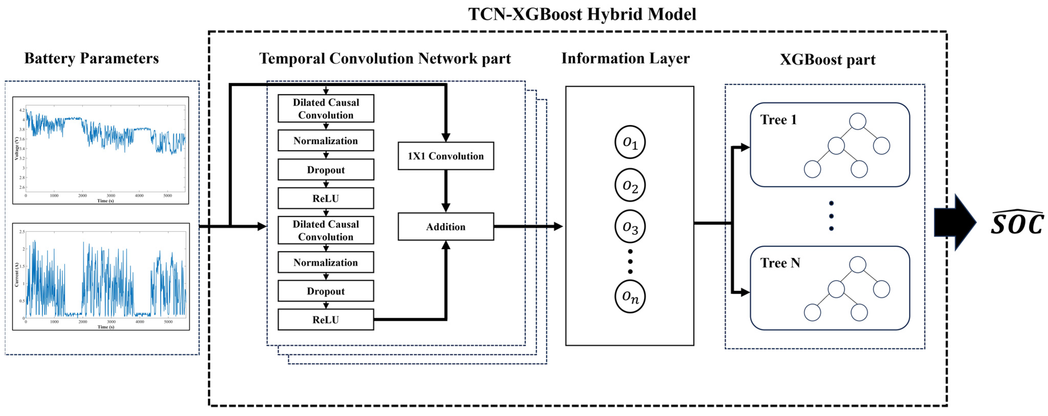
This hybrid model was designed to accurately estimate the SOC by receiving the internal parameters of a battery as sequence data from the TCN, extracting the characteristics of the data, and increasing the generalization performance by inputting the characteristics of the data into XGBoost. The structure of the proposed model is presented in Figure 3.
The battery parameters used as input to the proposed model using the NASA and Oxford datasets were discharge voltage, current, operation time, and temperature, while those using the vehicle simulator dataset were the discharge voltage of each cell, current, battery pack voltage, operation time, and temperature. The information layer transforms the output values of TCN into an input form for XGBoost. In the information layer, o 1 , …, o n represents the output values of TCN containing past information.
This model progresses through data preprocessing, feature extraction, past information usage, and generalization. Data preprocessing involves processing the dataset to standardize it and transform it into the appropriate format for input. Feature extraction uses residual blocks with dilated causal convolutions in TCN to extract features from the data using information from both the past and present, thereby creating long-effective memory features. To transmit the information from both past and present data from the output of TCN to the input of XGBoost, an information layer is defined. The information layer is responsible for configuring the number of input parameters when passing the output of the TCN to the XGBoost model and converting the 2D output of the TCN into a 1D format suitable for XGBoost input. The reason for configuring the number of input parameters is to enhance the prediction accuracy of XGBoost using the current input, including past information, as the input for XGBoost. In other words, if the information layer has two nodes, o n 2 , o n 1 , and o n are used as input to XGBoost when making predictions. Through the boosting algorithm, XGBoost sequentially trains multiple weak learners. By assigning weights to incorrectly predicted data and iteratively updating these weights, the weak learners are progressively strengthened, culminating in the formation of a final predictor, resulting in a more generalized and robust model. Subsequently, XGBoost estimates the SOC and outputs the result. Generalization involves transmitting the data from the information layer to XGBoost. Subsequently, XGBoost estimates the SOC and outputs the result.
Our battery SOC estimation process based on the proposed model is as follows:
  • To use the battery data as input to the proposed model, the data were set in sequence. Voltage, current, temperature, and operation time were used as input parameters.
  • The input data were used as the input for TCN, and the output of TCN was obtained using the dilated convolution operation in Equation (2) and the activation function in Equation (3). Herein, the ReLU function was used as the activation function.
  • The information layer determines how much past information from the output of TCN to use. For instance, if n pieces of past information are chosen, the sequential data o 1 , o 2 , …, o n 1 , o n are used as inputs for the subsequent XGBoost model.
  • The information layer transfers the data to XGBoost, and XGBoost ultimately estimates the SOC based on Equation (7).

3. Experiments and Results

In this study, the proposed model’s performance was evaluated through training on datasets from NASA, Oxford, and a vehicle simulator. The training was conducted on a computer equipped with a The AMD Ryzen 5600X processor from the United States, California, an The NVIDIA RTX 3070 graphics card from the United States, California, and 16 GB of RAM, using Python 3.6, TensorFlow 2.2, and the Keras library.
In the conducted experiments, a multilayer neural network (MNN) [33], long short-term memory (LSTM) [34], a gated recurrent unit (GRU) [35], XGBoost, and a temporal convolutional network (TCN) were employed to assess their performance in comparison to the proposed hybrid TCN-XGBoost model. The hyperparameters for each model used in the experiments are provided in Table 2.
For the TCN model in Table 2, nb_filter is the number of filters to use in the convolutional layers, kernal_size is the size of the kernel to use in each convolutional layer, nb_stack is the number of stacks of residual blocks to use, dilations is a dilation list, padding is the padding to use in the convolution, “causal” means a causal network, and use_skip_connections is the setting to add skip connections from the input to each residual block.
In the XGBoost model, ‘n_estimators’ represents the number of gradient-boosted trees, ‘max_depth’ is the maximum tree depth for base learners, ‘gamma’ signifies the minimum loss reduction required to initiate an additional partition on a leaf node of the tree, ‘reg_alpha’ and ‘reg_lambda’ denote L1 and L2 regularization terms applied to weights, and ‘subsample’ stands for the subsample ratio of the training instances.
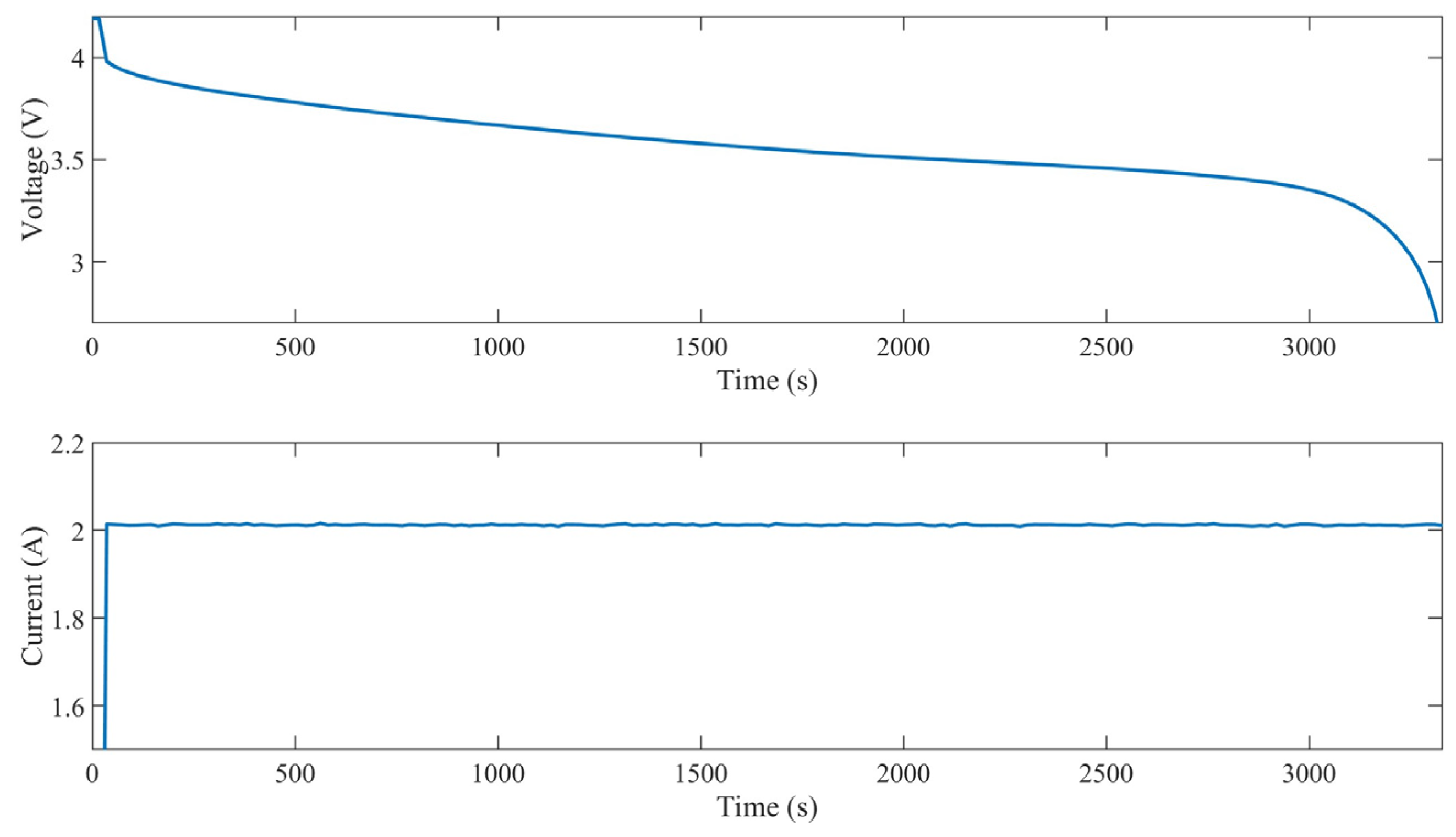
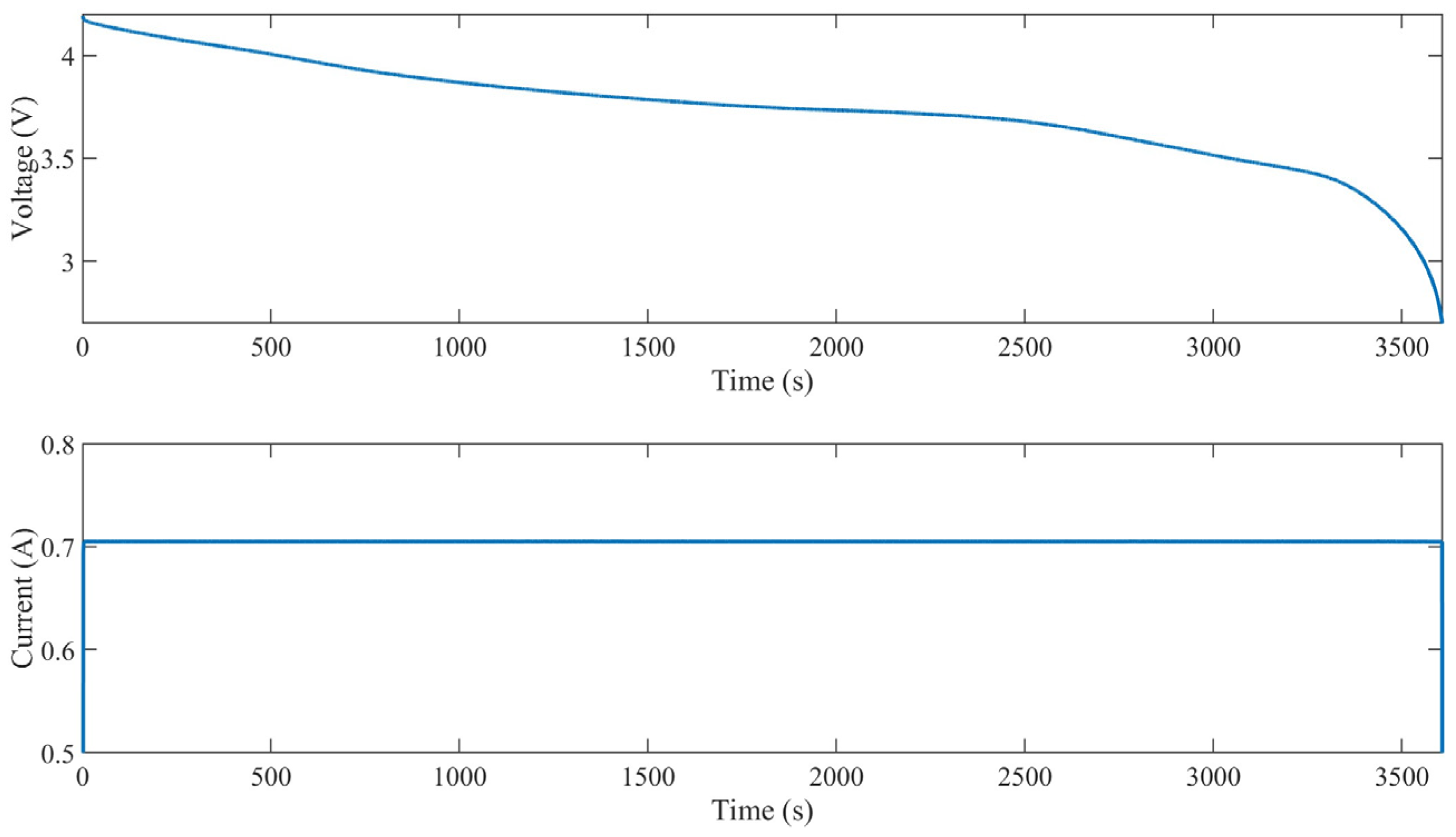
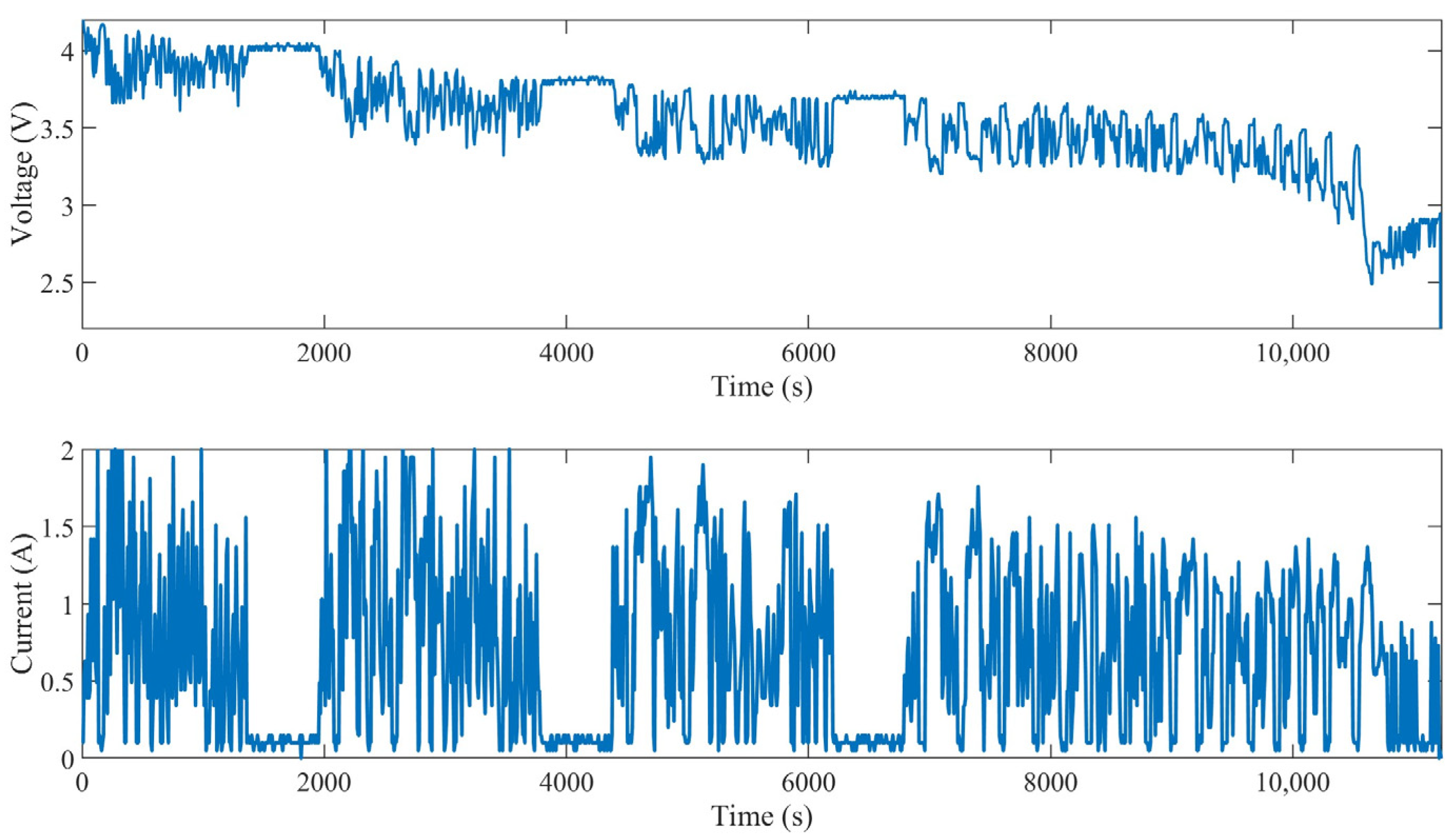
The experiments used battery data provided by the NASA Ames Research Center and Oxford. NASA’s battery dataset includes periodic charge and discharge cycles using lithium-ion 18650 batteries. These experiments yielded information on temperature, load voltage, current, and time. Charging was conducted at a constant current of 1.5 A until the battery voltage reached 4.2 V, while discharging proceeded at a constant current of 740 mA until reaching 2.7 V. Herein, data from Battery #5 were used. Oxford’s dataset includes periodic charge and discharge experiments using small lithium-ion pouch cells in a 40 °C environment, performed at constant current and constant voltage. In this study, data from Battery Cell 1 were used. The vehicle simulator dataset was generated by serially connecting eight lithium-ion 18650 battery cells and conducting discharge experiments using a vehicle simulator. This vehicle simulator was based on the The Hyundai Motor-manufactured Avante Sports AD 16 vehicle produced in Ulsan, South Koreaand was custom-built to match the wheel size and motor RPM specifications for the experiments. The vehicle simulator operated in FTP-75 mode, and the experiments continued until the battery pack was fully discharged. For the NASA dataset, the B0005 battery dataset was used, and a total of 6 and 144 cycles were used for the tests and learning, respectively. The Cell 2 battery dataset from the Oxford dataset was utilized, with a total of 6 cycles for testing and 71 cycles for training. In the case of the vehicle simulator dataset, 1 cycle was used for testing, and 10 cycles were used for training. The experimental data is visualized in Figure 4, Figure 5 and Figure 6.
The error was calculated using the mean absolute error, which is shown in the following equation:
M A E = 1 n i = 1 n y i y ^ ,
where n is the total number of parameters, y i is the target value, and y ^ is the estimated value.
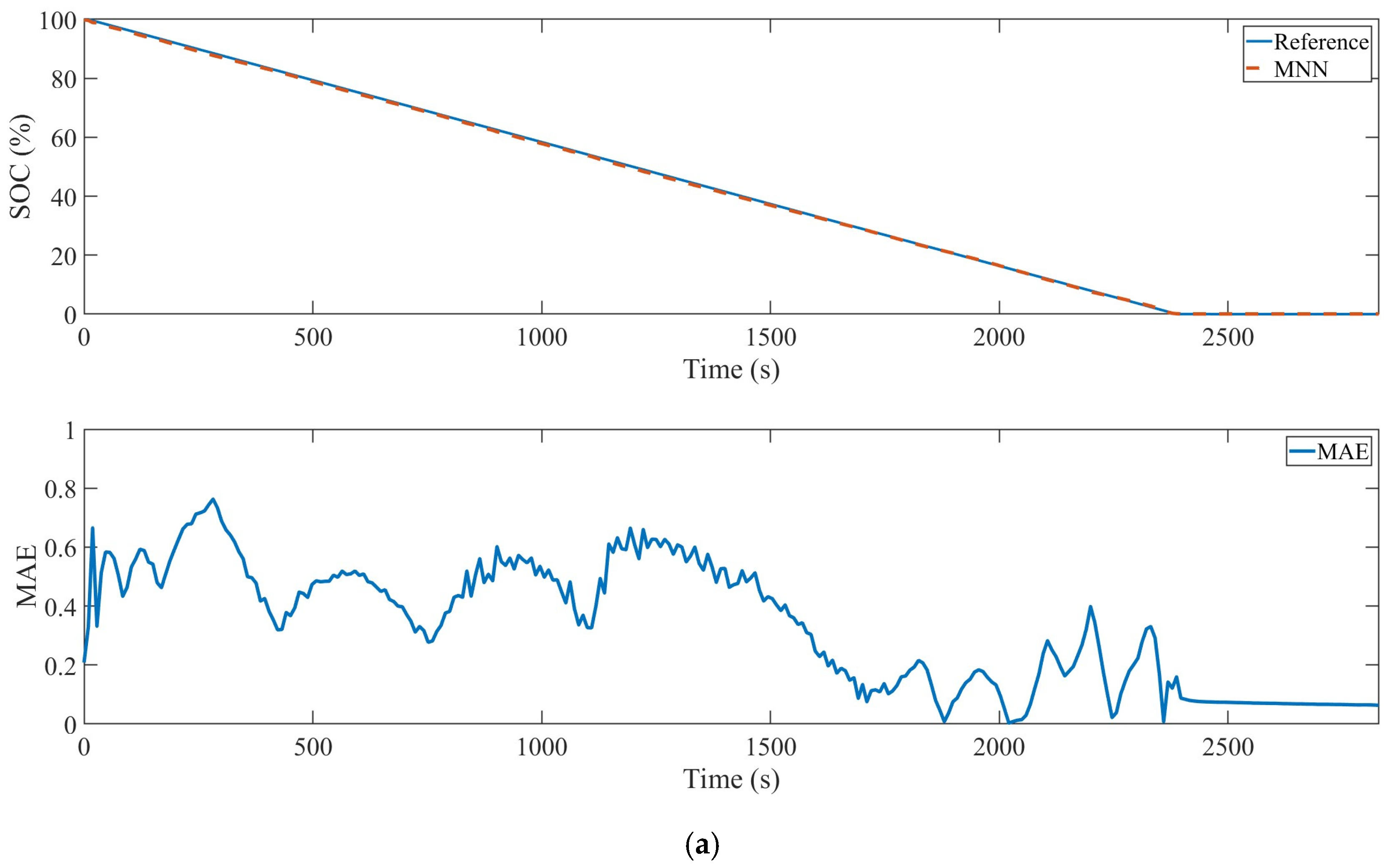
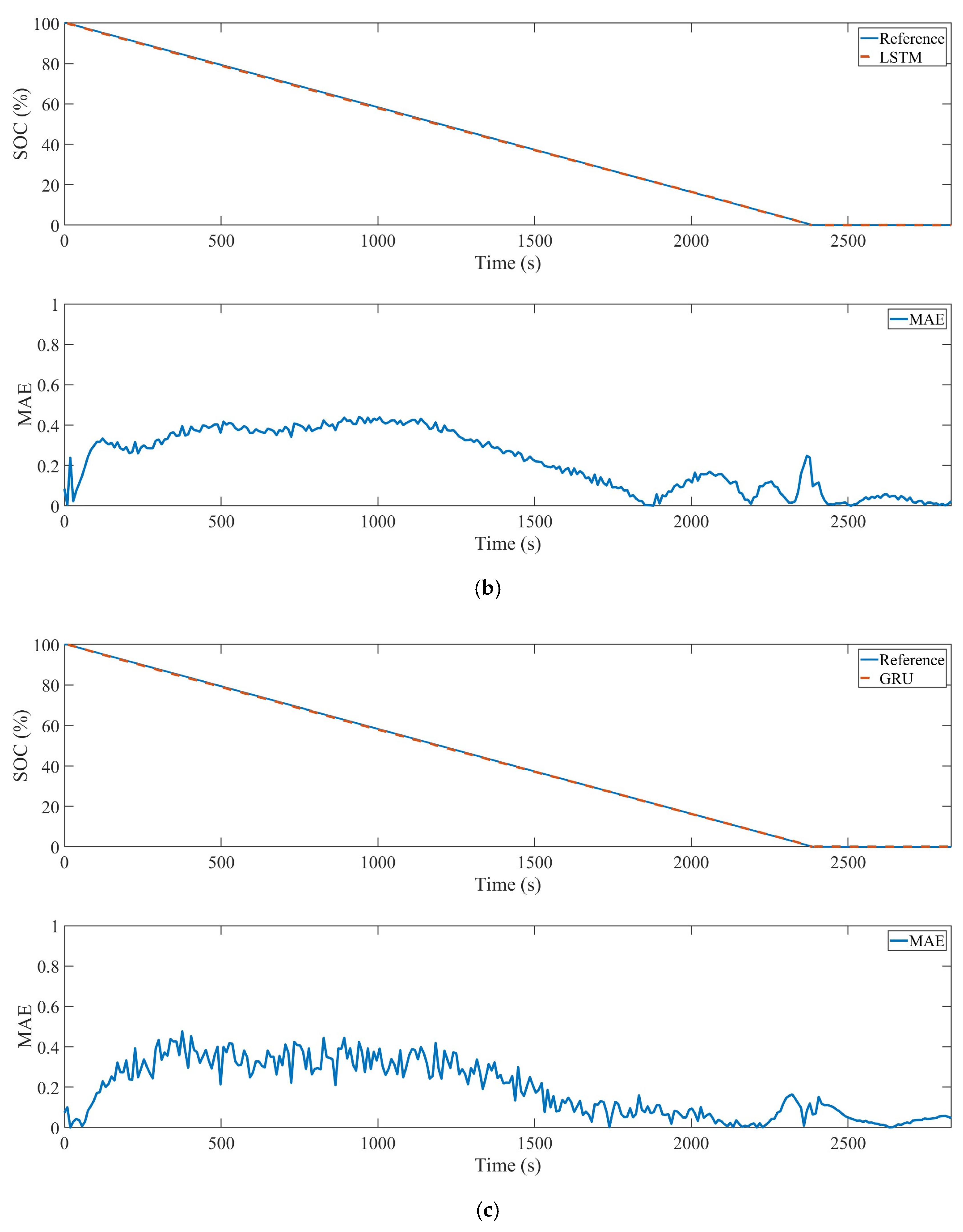
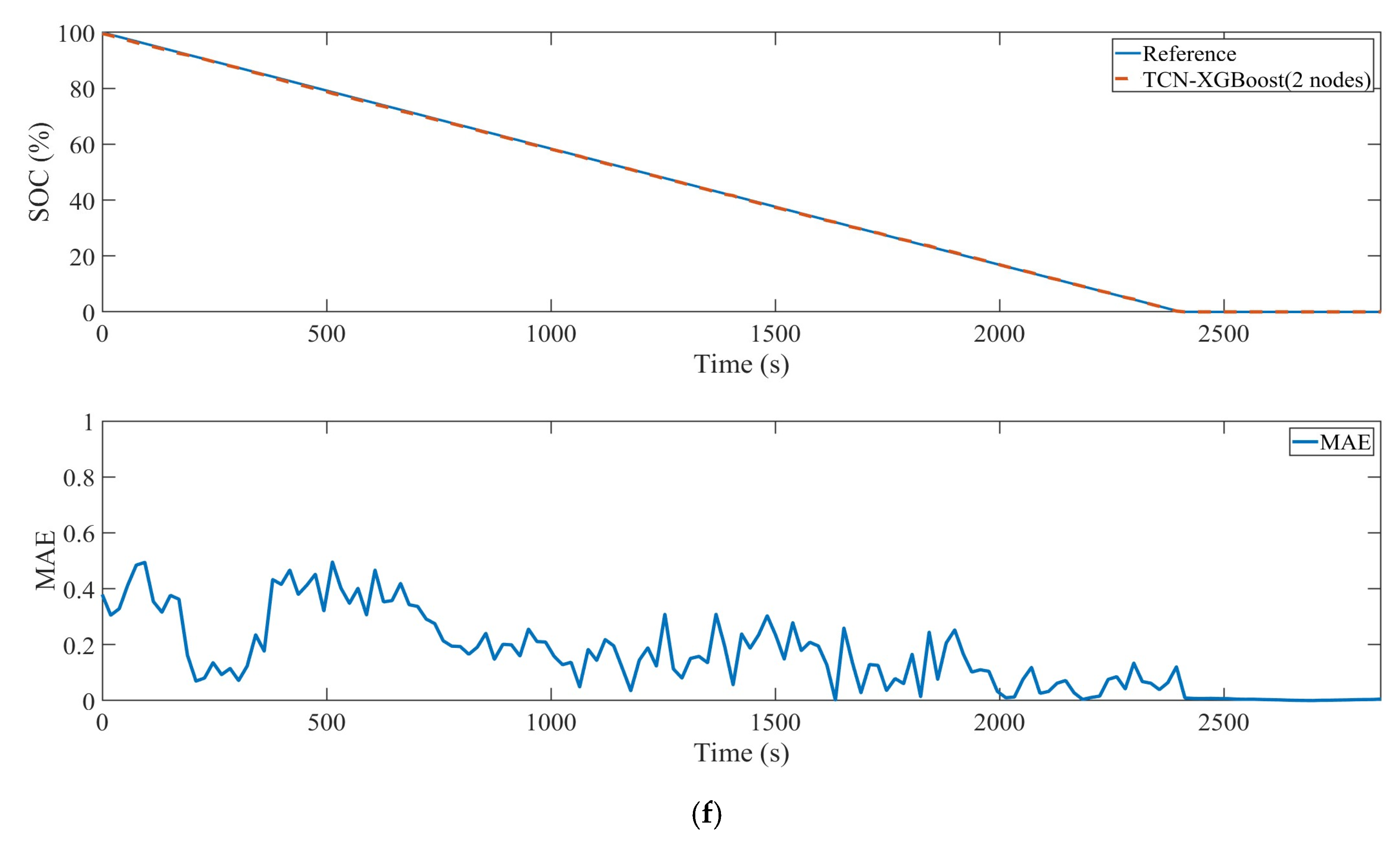
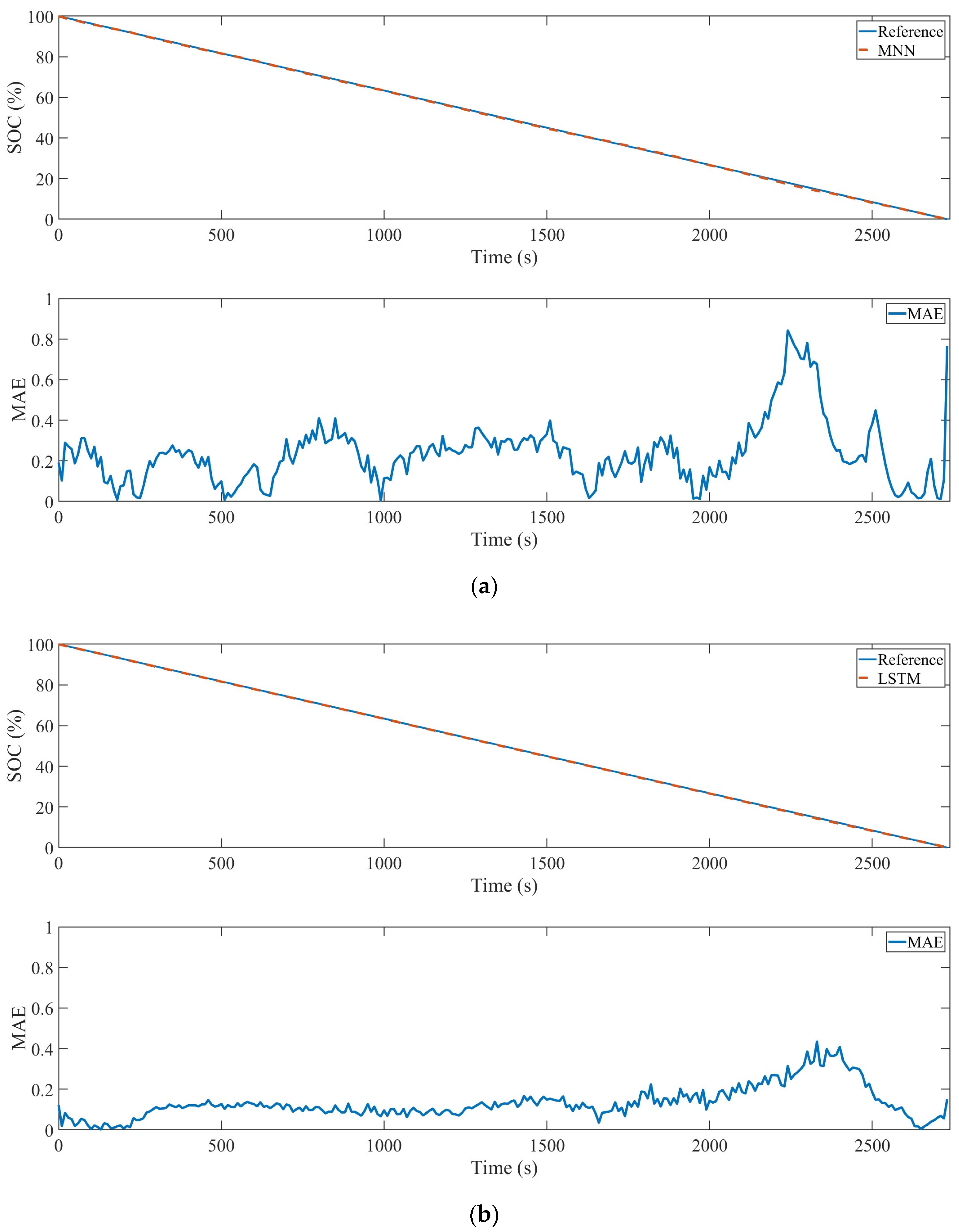
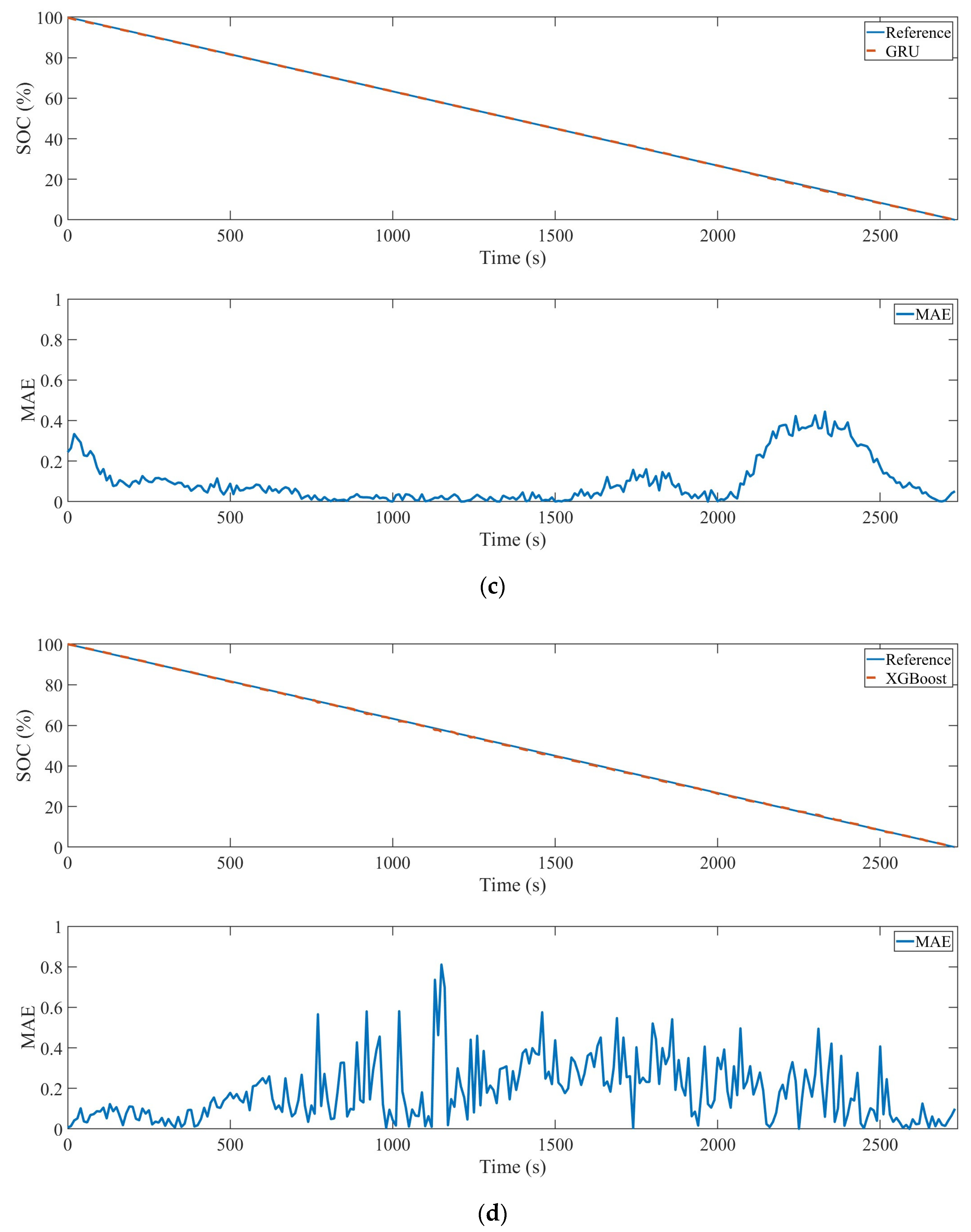
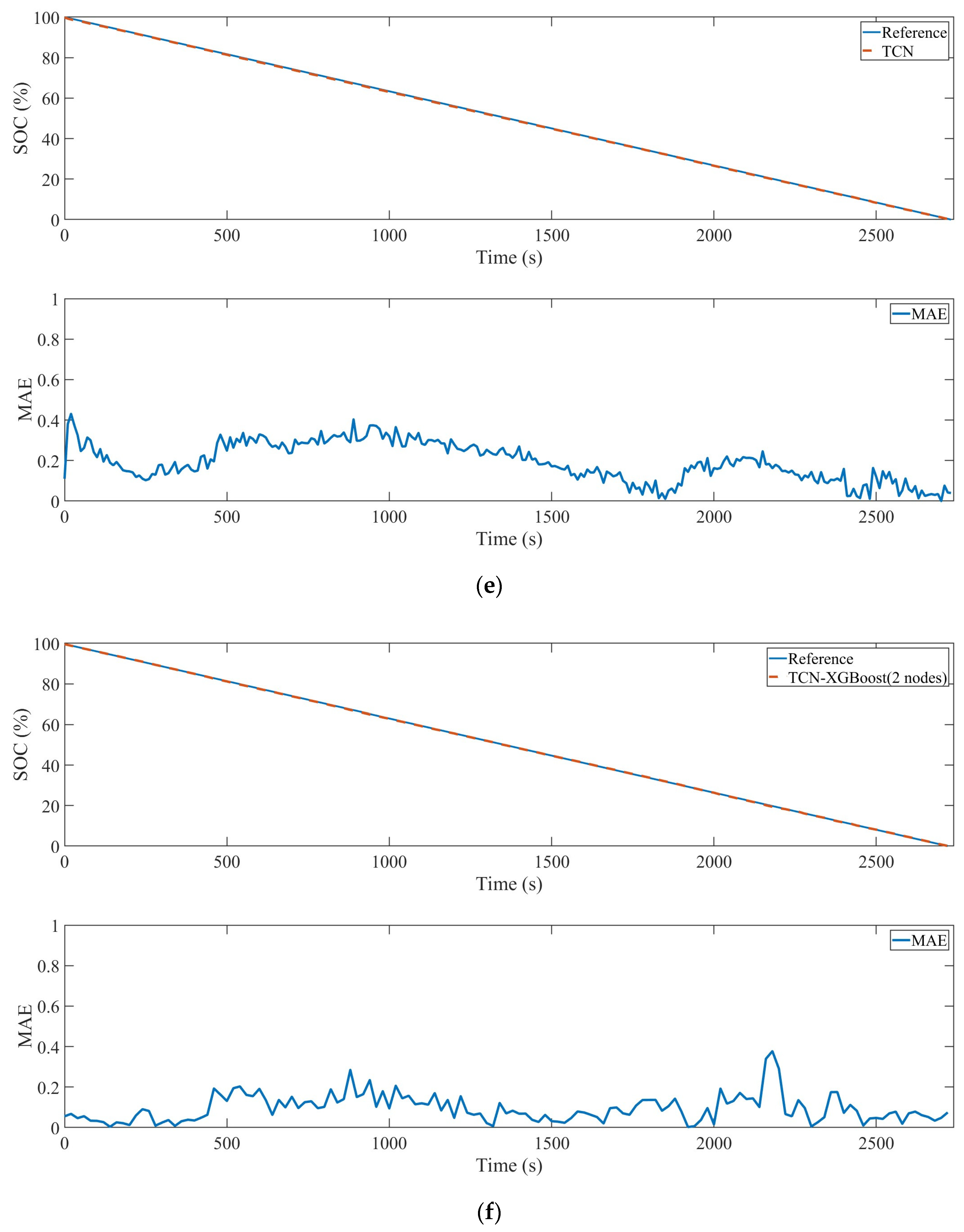
The experimental results obtained for each model using the NASA dataset are presented in Table 3. The mean absolute errors (MAEs) for MNN, LSTM, and GRU are 0.1408, 0.1296, and 0.1313, respectively. XGBoost and TCN exhibit MAEs of 0.1275 and 0.128, respectively, while TCN-XGBoost (one node) and TCN-XGBoost (two nodes) demonstrate MAEs of 0.1005 and 0.0955, respectively. The evaluation revealed that the SOC estimation by the proposed TCN-XGBoost hybrid model outperformed those by other models for 150 cycles, representing the battery test dataset under degraded conditions. Additionally, for the remaining NASA test dataset, the proposed model exhibited greater accuracy compared to the other models.
Figure 7 shows the SOC estimation results of each model used in the experiments and the results for 150 cycles using the NASA dataset. The upper graph presents the estimation results of the model, and the lower graph presents its estimation error.
The experimental results obtained using the Oxford dataset indicate that the MAEs for MNN, LSTM, and GRU are 0.2105, 0.1563, and 0.1253, respectively (Table 4). XGBoost and TCN exhibit MAEs of 0.142 and 0.1767, while TCN-XGBoost (one node) and TCN-XGBoost (two nodes) demonstrate average estimation errors of 0.1003 and 0.0983, respectively. The proposed TCN-XGBoost hybrid model, incorporating the information layer, achieves an MAE of 0.0983. When comparing the proposed model to MNN, the difference in MAE is 0.112. Notably, the error is lower than that of the existing TCN and XGBoost models, indicating good estimation performance of the TCN-XGBoost model with the information layer when using the Oxford dataset. Figure 8 depicts the SOC estimation results of each model employed in the experiments and the results for 78 cycles using the Oxford dataset.
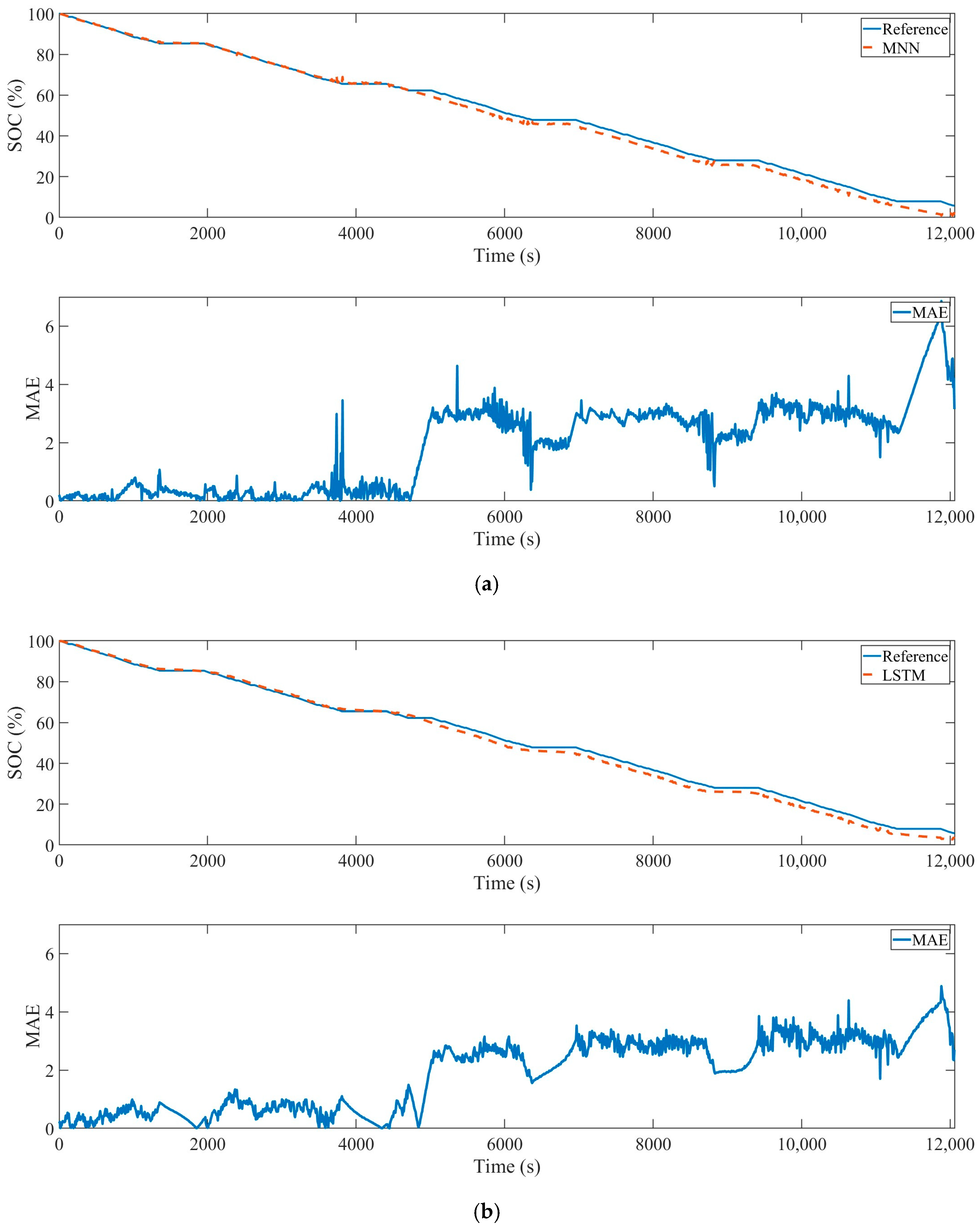
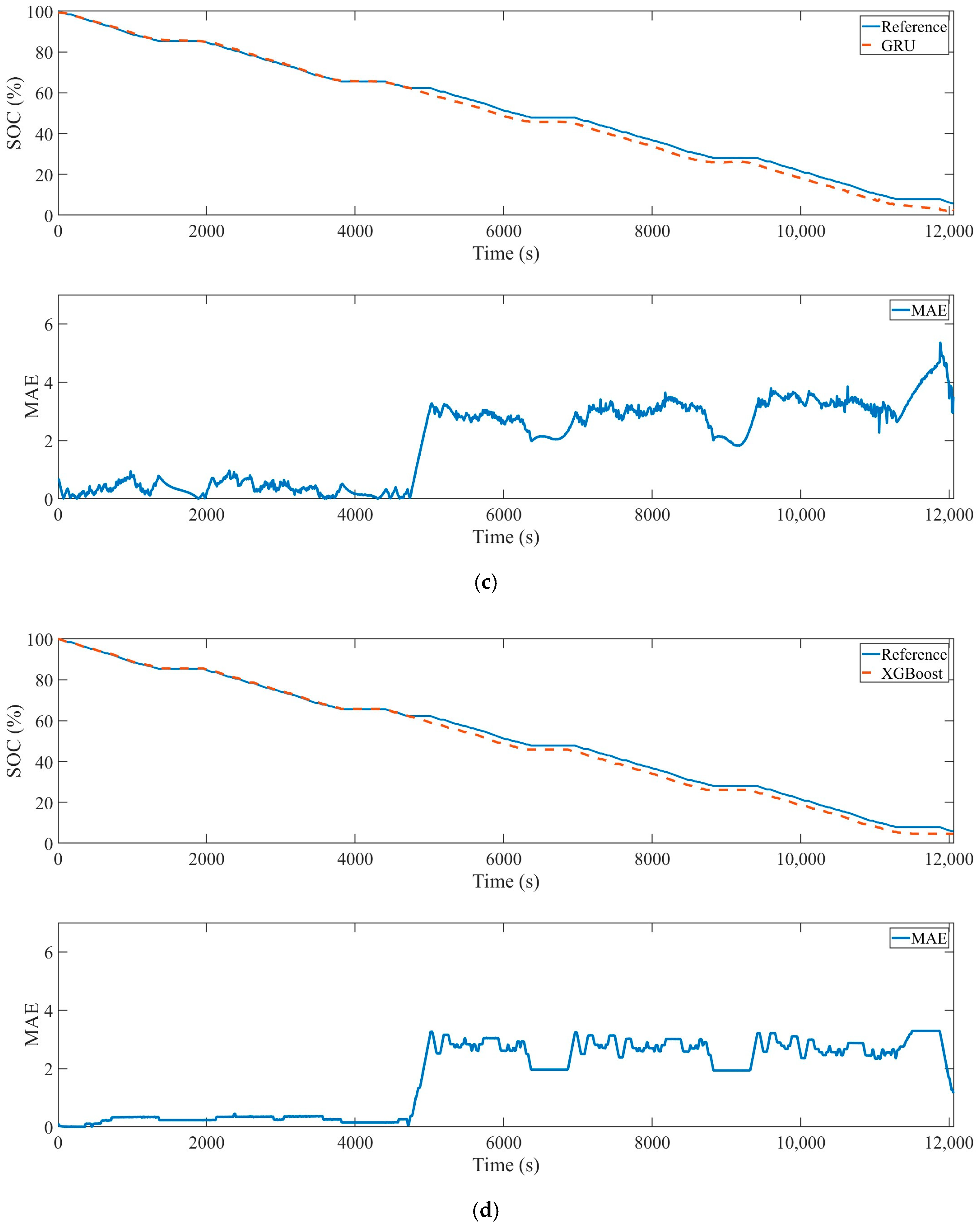
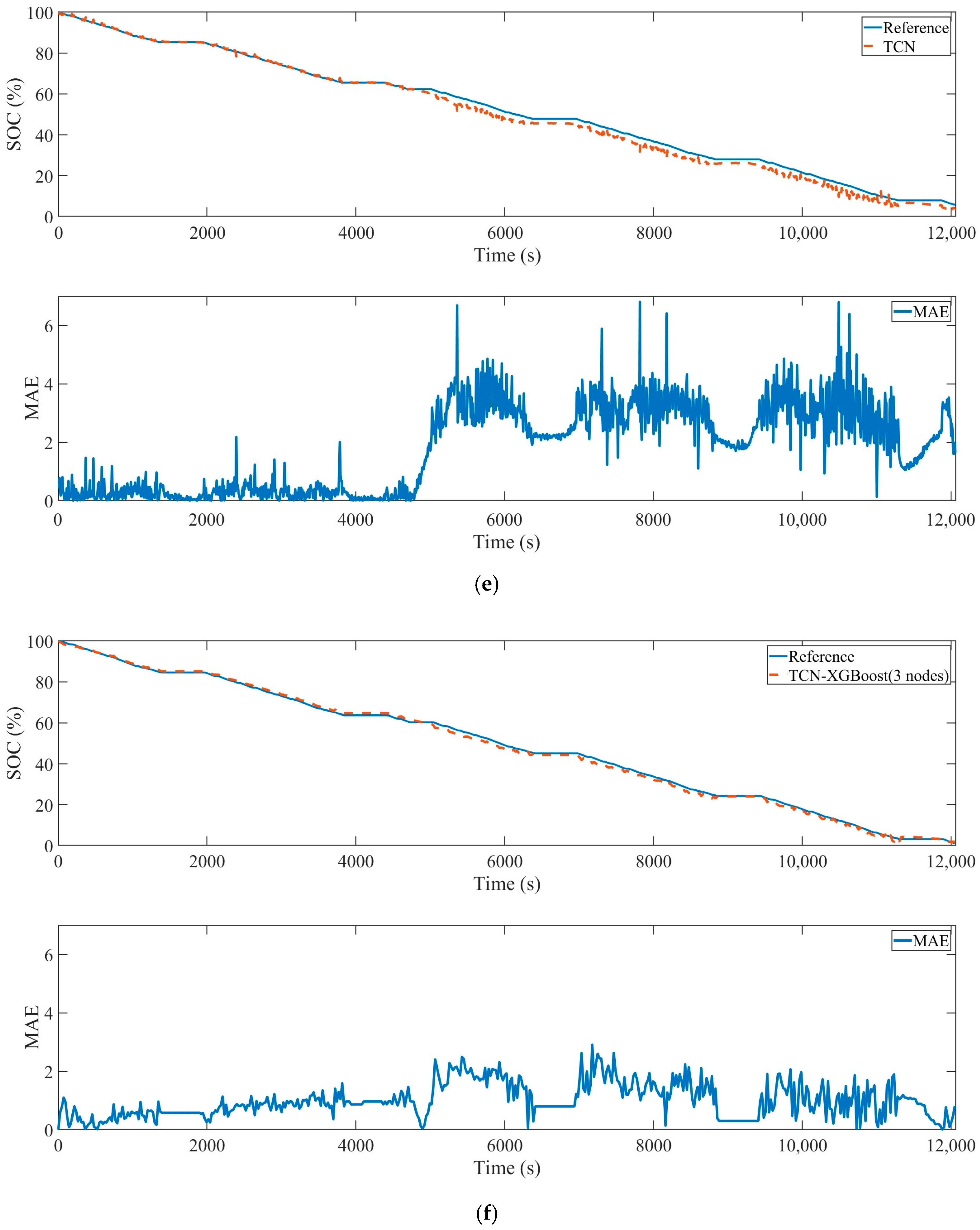
Table 5 presents the results obtained from experiments conducted using the vehicle simulator dataset. MNN, LSTM, and GRU demonstrate MAEs of 1.857, 1.624, and 1.648, respectively. XGBoost and TCN exhibit MAEs of 1.456 and 1.393, while TCN-XGBoost (one node), TCN-XGBoost (two nodes), and TCN-XGBoost (three nodes) achieve MAEs of 1.413, 1.386, and 1.381, respectively. Despite the frequent data fluctuations in the vehicle simulator dataset, the proposed model outperforms the other models. Figure 9 depicts the SOC estimation results for each model used in the experiments and the results for cell 7 using the vehicle simulator dataset.
To validate the performance of our proposed model, we compared its results with those of other battery SOC estimation studies [36,37] that used data from Battery #5 in the NASA dataset. Zhang et al. [36] proposed an SOH–SOC simultaneous estimation model based on the GWO-BP neural network. The algorithm in [36] exhibited an average SOC estimation error within 5%. The model presented in our paper demonstrates battery SOC estimation with an accuracy of <1%, indicating its ease of use compared to BP-based models [36]. Furthermore, Li et al. [37] estimated battery SOC using the FCNN, 2DCNN, and 3DCNN models based on CNN. Among the proposed models, FCNN achieved the best performance, with a MAE of 0.4694. The model proposed in this paper shows easy battery SOC estimation, with an MAE of 0.095.

4. Conclusions

This paper proposes a hybrid TCN-XGBoost model for estimating the SOC of lithium batteries. The proposed model integrates a TCN with long-effective memory features, leverages XGBoost for enhanced estimation performance, and incorporates an information layer to use past information as the next input. Within this framework, the TCN extracts data features, while the information layer sequentially transforms past information into a 1D matrix. XGBoost is employed to optimize the model structure to effectively align it with the extracted features. Experimental results validate that the proposed model effectively captures battery SOC characteristics, resulting in improved estimation accuracy.
For the validation of the proposed model, MNN, LSTM, and GRU were employed. TCN and XGBoost were also used to compare the performance of single and hybrid models. Furthermore, to validate the proposed model across diverse battery characteristics, battery data from the NASA, Oxford, and vehicle simulator datasets were employed. Experimental results indicate that the proposed model outperformed the other models, with MAEs of 0.095, 0.0983, and 1.381 using the NASA, Oxford, and vehicle simulator test datasets, respectively, confirming its superior estimation performance. Moreover, the proposed model exhibited superior estimation performance to single models, underscoring the effectiveness of the model.
In future research, we plan to apply the proposed model to a real-world environment to evaluate its practical utility.

Author Contributions

Formal analysis, J.-H.L. and I.-S.L.; investigation, J.-H.L.; algorithm, J.-H.L. and I.-S.L.; experiment and simulation, J.-H.L.; validation, J.-H.L. and I.-S.L.; writing—original draft preparation, J.-H.L.; writing—review and editing, J.-H.L. and I.-S.L. All authors have read and agreed to the published version of the manuscript.

Funding

This research was funded by the Ministry of Education (Korea) under the BK21 FOUR project, grant number 4199990113966.

Data Availability Statement

Publicly available datasets were analyzed in this study. These data can be found at https://www.nasa.gov/intelligent-systems-division/discovery-and-systems-health/pcoe/pcoe-data-set-repository/ (accessed on 22 December 2021) and https://ora.ox.ac.uk/objects/uuid:03ba4b01-cfed-46d3-9b1a7d4a7bdf6fac (accessed on 22 December 2021).

Conflicts of Interest

The authors declare no conflict of interest.

References

  1. Chen, J.; Zhang, Y.; Wu, J.; Cheng, W.; Zhu, Q. SOC estimation for lithium-ion battery using the LSTM-RNN with extended input and constrained output. Energy 2023, 262, 125375. [Google Scholar] [CrossRef]
  2. Luo, K.; Chen, X.; Zheng, H.; Shi, Z. A review of deep learning approach to predicting the state of health and state of charge of lithium-ion batteries. J. Energy Chem. 2022, 74, 159–173. [Google Scholar] [CrossRef]
  3. Lai, X.; Yao, J.; Jin, C.; Feng, X.; Wang, H.; Xu, C.; Zheng, Y. A review of lithium-ion battery failure hazards: Test standards, accident analysis, and safety suggestions. Batteries 2022, 8, 248. [Google Scholar] [CrossRef]
  4. Wang, Q.; Mao, B.; Stoliarov, S.I.; Sun, J. A review of lithium ion battery failure mechanisms and fire prevention strategies. Prog. Energy Combust. Sci. 2019, 73, 95–131. [Google Scholar] [CrossRef]
  5. Park, J.H.; Lee, J.H.; Kim, S.J.; Lee, I.S. Real-time state of charge estimation for each cell of lithium battery pack using neural networks. Appl. Sci. 2020, 10, 8644. [Google Scholar] [CrossRef]
  6. Seh, Z.W.; Sun, Y.; Zhang, Q.; Cui, Y. Designing high-energy lithium–sulfur batteries. Chem. Soc. Rev. 2016, 45, 5605–5634. [Google Scholar] [CrossRef]
  7. Xiong, R.; Li, L.; Tian, J. Towards a smarter battery management system: A critical review on battery state of health monitoring methods. J. Power Sources 2018, 405, 18–29. [Google Scholar] [CrossRef]
  8. Shen, M.; Gao, Q. A review on battery management system from the modeling efforts to its multiapplication and integration. Int. J. Energy Res. 2019, 43, 5042–5075. [Google Scholar] [CrossRef]
  9. Yang, B.; Wang, J.; Cao, P.; Zhu, T.; Shu, H.; Chen, J.; Zhang, J.; Zhu, J. Classification, summarization and perspectives on state-of-charge estimation of lithium-ion batteries used in electric vehicles: A critical comprehensive survey. J. Energy Storage 2021, 39, 102572. [Google Scholar] [CrossRef]
  10. Wang, Y.; Tian, J.; Sun, Z.; Wang, L.; Xu, R.; Li, M.; Chen, Z. A comprehensive review of battery modeling and state estimation approaches for advanced battery management systems. Renew. Sustain. Energy Rev. 2020, 131, 110015. [Google Scholar] [CrossRef]
  11. How, D.N.T.; Hannan, M.A.; Hossain Lipu, M.S.; Ker, P.J. State of charge estimation for lithium-ion batteries using model-based and data-driven methods: A review. IEEE Access 2019, 7, 136116–136136. [Google Scholar] [CrossRef]
  12. Corno, M.; Bhatt, N.; Savaresi, S.M.; Verhaegen, M. Electrochemical model-based state of charge estimation for Li-ion cells. IEEE Trans. Control Syst. Technol. 2014, 23, 117–127. [Google Scholar] [CrossRef]
  13. He, H.; Xiong, R.; Fan, J. Evaluation of lithium-ion battery equivalent circuit models for state of charge estimation by an experimental approach. Energies 2011, 4, 582–598. [Google Scholar] [CrossRef]
  14. Sun, F.; Hu, X.; Zou, Y.; Li, S. Adaptive unscented Kalman filtering for state of charge estimation of a lithium-ion battery for electric vehicles. Energy 2011, 36, 3531–3540. [Google Scholar] [CrossRef]
  15. Wu, B.; Han, S.; Shin, K.G.; Lu, W. Application of artificial neural networks in design of lithium-ion batteries. J. Power Sources 2018, 395, 128–136. [Google Scholar] [CrossRef]
  16. Chemali, E.; Kollmeyer, P.J.; Preindl, M.; Ahmed, R.; Emadi, A. Long short-term memory networks for accurate state-of-charge estimation of Li-ion batteries. IEEE Trans. Ind. Electron. 2017, 65, 6730–6739. [Google Scholar] [CrossRef]
  17. Shen, P.; Ouyang, M.; Lu, L.; Li, J.; Feng, X. The co-estimation of state of charge, state of health, and state of function for lithium-ion batteries in electric vehicles. IEEE Trans. Veh. Technol. 2017, 67, 92–103. [Google Scholar] [CrossRef]
  18. Barai, A.; Widanage, W.D.; Marco, J.; McGordon, A.; Jennings, P. A study of the open circuit voltage characterization technique and hysteresis assessment of lithium-ion cells. J. Power Sources 2015, 295, 99–107. [Google Scholar] [CrossRef]
  19. Ng, M.F.; Zhao, J.; Yan, Q.; Conduit, G.J.; Seh, Z.W. Predicting the state of charge and health of batteries using data-driven machine learning. Nat. Mach. Intell. 2020, 2, 161–170. [Google Scholar] [CrossRef]
  20. Severson, K.A.; Attia, P.M.; Jin, N.; Perkins, N.; Jiang, B.; Yang, Z.; Chen, M.H.; Aykol, M.; Herring, P.K.; Fraggedakis, D.; et al. Data-driven prediction of battery cycle life before capacity degradation. Nat. Energy 2019, 4, 383–391. [Google Scholar] [CrossRef]
  21. Attia, P.M.; Grover, A.; Jin, N.; Severson, K.A.; Markov, T.M.; Liao, Y.H.; Chen, M.H.; Cheong, B.; Perkins, N.; Yang, Z.; et al. Closed-loop optimization of fast-charging protocols for batteries with machine learning. Nature 2020, 578, 397–402. [Google Scholar] [CrossRef] [PubMed]
  22. Ng, K.S.; Moo, C.S.; Chen, Y.P.; Hsieh, Y. Enhanced coulomb counting method for estimating state-of-charge and state-of-health of lithium-ion batteries. Appl. Energy 2009, 86, 1506–1511. [Google Scholar] [CrossRef]
  23. Truchot, C.; Dubarry, M.; Liaw, B.Y. State-of-charge estimation and uncertainty for lithium-ion battery strings. Appl. Energy 2014, 119, 218–227. [Google Scholar] [CrossRef]
  24. Jang, K.W.; Chung, G.B. A SOC estimation using Kalman filter for lithium-polymer battery. Trans. Korean Inst. Power Electron. 2012, 17, 222–229. [Google Scholar] [CrossRef]
  25. Xiong, R.; Sun, F.; Chen, Z.; He, H. A data-driven multi-scale extended Kalman filtering based parameter and state estimation approach of lithium-ion polymer battery in electric vehicles. Appl. Energy 2014, 113, 463–476. [Google Scholar] [CrossRef]
  26. Rzepka, B.; Bischof, S.; Blank, T. Implementing an extended Kalman filter for SoC estimation of a Li-ion battery with hysteresis: A step-by-step guide. Energies 2021, 14, 3733. [Google Scholar] [CrossRef]
  27. Li, J.; Ye, M.; Gao, K.; Xu, X.; Wei, M.; Jiao, S. Joint estimation of state of charge and state of health for lithium-ion battery based on dual adaptive extended Kalman filter. Int. J. Energy Res. 2021, 45, 13307–13322. [Google Scholar] [CrossRef]
  28. Chemali, E.; Kollmeyer, P.J.; Preindl, M.; Emadi, A. State-of-charge estimation of Li-ion batteries using deep neural networks: A machine learning approach. J. Power Sources 2018, 400, 242–255. [Google Scholar] [CrossRef]
  29. Bai, S.; Kolter, J.Z.; Koltun, V. An empirical evaluation of generic convolutional and recurrent networks for sequence modelling. arXiv 2018, arXiv:1803.01271. [Google Scholar]
  30. Li, L.; Li, Y.; Mao, R.; Li, L.; Hua, W.; Zhang, J. Remaining useful life prediction for lithium-ion batteries with a hybrid model based on TCN-GRU-DNN and dual attention mechanism. IEEE Trans. Transp. Electrif. 2023, 9, 4726–4740. [Google Scholar] [CrossRef]
  31. Tianqi, C.; Carlos, G. Xgboost: A scalable tree boosting system. In Proceedings of the 22nd ACM SIGKDD International Conference on Knowledge Discovery and Data Mining, San Francisco, CA, USA, 13–17 August 2016; pp. 785–794. [Google Scholar]
  32. An, J.; Guo, W.; Lv, T.; Zhao, Z.; He, C.; Zhao, H. Joint prediction of the state of charge and the state of health of lithium-ion batteries based on the PSO-XGBoost algorithm. Energies 2023, 16, 4243. [Google Scholar] [CrossRef]
  33. Popescu, M.C.; Balas, V.E.; Perescu-Popescu, L.; Mastorakis, N. Multilayer Perceptron and neural networks. WSEAS Trans. Circuits Syst. 2009, 8, 579–588. [Google Scholar]
  34. Staudemeyer, R.C.; Morris, E.R. Understanding LSTM—A tutorial into long short-term memory recurrent neural networks. arXiv 2019, arXiv:1909.09586. [Google Scholar]
  35. Cho, K.; Van Merriënboer, B.; Gulcehre, C.; Bahdanau, D.; Bougares, F.; Schwenk, H.; Bengio, Y. Learning phrase representations using rnn encoder-decoder for statistical machine translation. arXiv 2014, arXiv:1406.1078. [Google Scholar]
  36. Zhang, X.; Hou, J.; Wang, Z.; Jiang, Y. Joint SOH-SOC estimation model for lithium-ion batteries based on GWO-BP neural network. Energies 2022, 16, 132. [Google Scholar] [CrossRef]
  37. Li, J.; Jiang, Z.; Jiang, Y.; Song, W.; Gu, J. The state of charge estimation of lithium-ion battery based on battery capacity. J. Electrochem. Soc. 2022, 169, 120539. [Google Scholar] [CrossRef]
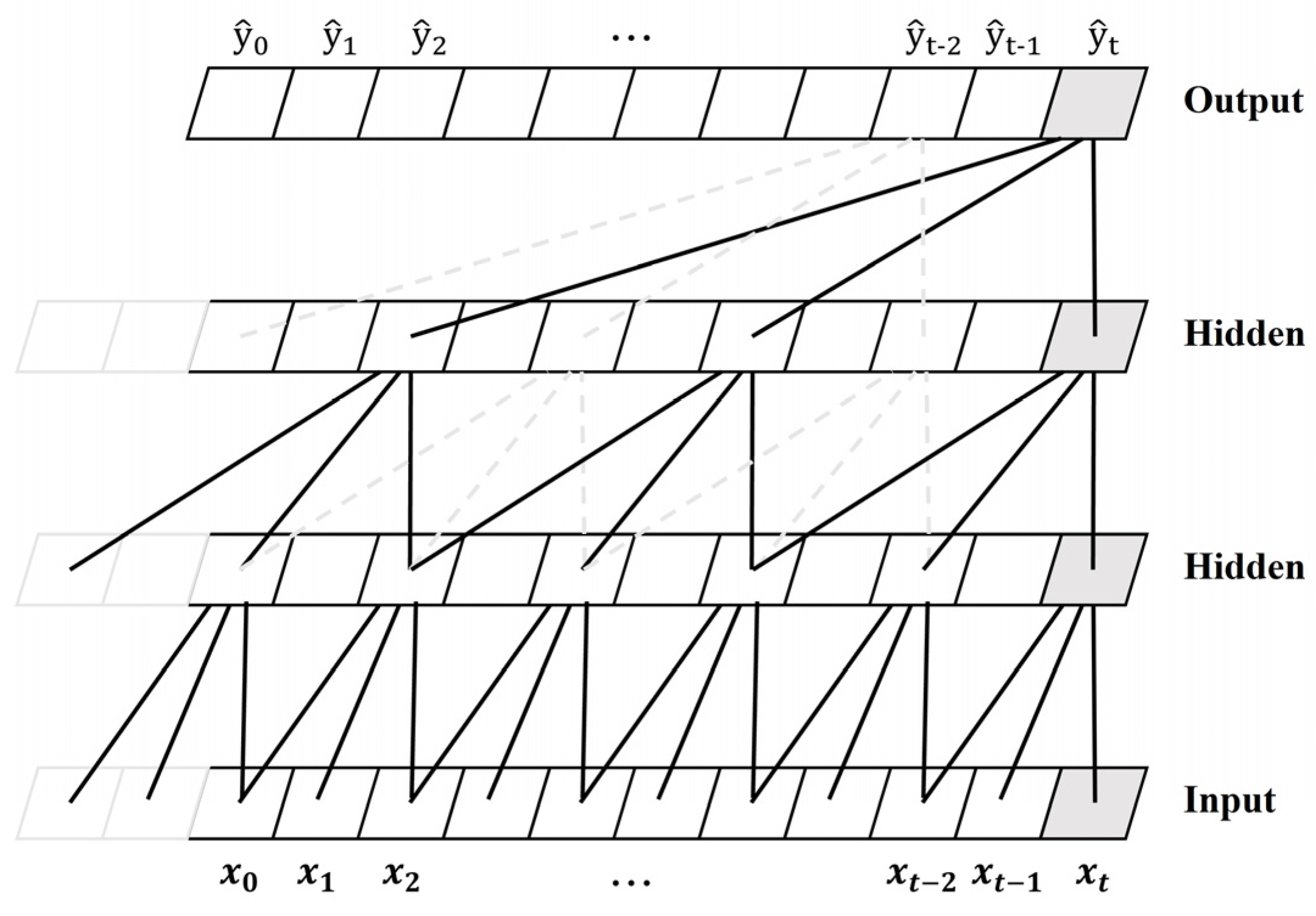
Figure 1. Dilated causal convolution.
Batteries 09 00544 g001
Figure 2. TCN residual block.
Batteries 09 00544 g002
Figure 3. Structure of the proposed TCN-XGBoost hybrid model.
Batteries 09 00544 g003
Figure 4. NASA battery voltage and current data used in the experiments.
Batteries 09 00544 g004
Figure 5. Oxford battery voltage and current data used in the experiments.
Batteries 09 00544 g005
Figure 6. Voltage and current of the cell of the vehicle simulator battery pack used in the experiments.
Batteries 09 00544 g006
Figure 7. SOC estimation results and mean absolute error of each model for 150 cycles using the NASA dataset. (a) MNN, (b) LSTM, (c) GRU, (d) XGBoost, (e) TCN, and (f) TCN-XGBoost (two nodes).
Batteries 09 00544 g007aBatteries 09 00544 g007bBatteries 09 00544 g007cBatteries 09 00544 g007d
Figure 8. SOC estimation results and mean absolute error of each model for 78 cycles using the Oxfrod dataset. (a) MNN, (b) LSTM, (c) GRU, (d) XGBoost, (e) TCN, and (f) TCN-XGBoost (two nodes).
Batteries 09 00544 g008aBatteries 09 00544 g008bBatteries 09 00544 g008c
Figure 9. SOC estimation results and mean absolute error of each model for cell 7 using the vehicle simulator dataset. (a) MNN, (b) LSTM, (c) GRU, (d) XGBoost, (e) TCN, and (f) TCN-XGBoost (three nodes).
Batteries 09 00544 g009aBatteries 09 00544 g009bBatteries 09 00544 g009c
Table 1. Advantages and disadvantages of model-based, data-driven, and Coulomb counting methods.
MethodAdvancementsLimitationsExemplary Model
Model-based
[12,13]
1. Reliability and precision
2. Broad applicability
1. Demands substantial domain expertise
2. Involves a protracted development period
1. Equivalent circuit model
2. Electrochemical model
3. Kalman filter
Data-driven
[14,15,16,17,18,19,20,21]
1. Rapid development time
2. Minimal need for specialized knowledge
1. Demands a significant volume of data1. Neural network
2. Deep learning
3. Look-up table
Coulomb counting
[22,23]
Easy to implementAccumulation of errors occurs over timeCoulomb counting
Table 2. Hyperparameter settings for each model used in the experiments.
ModelHyperparameterValue
TCNnb_filter128
kernal_size3
nb_stack2
deliations[1,2,4,8,16,32]
paddingCausal
use_skip_conectionsTure
XGBoostn_estimators1000
max_depth5
gamma0
reg_alpha0
reg_lamda1
subsample0.75
learning rate0.001
MNNhidden layer, one node64
hidden layer, two nodes32
learning rate0.01
LSTMLSTM layer, one node32
LSTM layer, two nodes16
learning rate0.01
GRUGRU layer, one node32
GRU layer, two nodes16
learning rate0.01
Table 3. SOC estimation results of each model for the mean absolute error using the NASA dataset.
41 Cycle63 Cycle78 Cycle100 Cycle125 Cycle150 CycleAverage
MNN0.0760.1010.0830.1360.1150.3340.1408
LSTM0.090.1410.0960.1030.1260.2220.1296
GRU0.1850.0840.1310.1340.0660.1880.1313
XGBoost0.1760.0970.0830.0930.0880.2280.1275
TCN0.1260.1170.1250.1050.0980.1970.128
TCN-XGBoost
(one node)
0.1120.0810.0930.0780.0670.1720.1005
TCN-XGBoost
(two nodes)
0.0930.0800.0940.0810.0630.1620.0955
Table 4. SOC estimation results of each model for the mean absolute error using the Oxford dataset.
6 Cycle15 Cycle28 Cycle42 Cycle70 Cycle78 CycleAverage
MNN0.3030.2050.1640.1910.1670.2330.2105
LSTM0.2690.0880.1450.1820.1220.1320.1563
GRU0.210.1030.1150.1320.0950.0970.1253
XGBoost0.1020.1260.1980.1190.1460.1610.142
TCN0.1630.120.2030.1610.2220.1910.1767
TCN-XGBoost
(one node)
0.1160.0450.1350.0920.1230.0910.1003
TCN-XGBoost
(two nodes)
0.1130.0490.1340.0900.1100.0940.0983
Table 5. Results of each model for the SOC estimation error using the vehicle simulator dataset.
Cell 1Cell 2Cell 3Cell 4Cell 5Cell 6Cell 7Cell 8Average
MNN3.1731.361.1542.7721.9891.0081.8621.5451.857
LSTM2.6161.1370.742.3871.9091.0351.8771.2971.624
GRU2.6851.0350.7722.621.7311.081.9331.3311.648
XGBoost1.2351.2190.7452.361.6990.9911.6861.7151.456
TCN0.9571.2190.9342.2531.6040.951.7971.4281.393
TCN-XGBoost
(one node)
1.1431.140.9382.3331.5981.0281.7121.5141.413
TCN-XGBoost
(two nodes)
1.1211.1140.9372.2121.5691.0111.6671.4591.386
TCN-XGBoost
(three nodes)
1.1071.1270.922.2111.570.9971.6721.4411.381
Disclaimer/Publisher’s Note: The statements, opinions and data contained in all publications are solely those of the individual author(s) and contributor(s) and not of MDPI and/or the editor(s). MDPI and/or the editor(s) disclaim responsibility for any injury to people or property resulting from any ideas, methods, instructions or products referred to in the content.