Online State-of-Health Estimation for Fast-Charging Lithium-Ion Batteries Based on a Transformer–Long Short-Term Memory Neural Network

Abstract

With the rapid development of machine learning and cloud computing, deep learning methods based on big data have been widely applied in the assessment of lithium-ion battery health status. However, enhancing the accuracy and robustness of assessment models remains a challenge. This study introduces an innovative T-LSTM prediction network. Initially, a one-dimensional convolutional neural network (1DCNN) is employed to effectively extract local and global features from raw battery data, providing enriched inputs for subsequent networks. Subsequently, LSTM and transformer models are ingeniously combined to fully utilize their unique advantages in sequence modeling, further enhancing the accurate prediction of battery health status. Experiments were conducted using both proprietary and open-source datasets, and the results validated the accuracy and robustness of the proposed method. The experimental results on the proprietary dataset show that the T-LSTM-based estimation method exhibits excellent performance in various evaluation metrics, with MSE, RMSE, MAE, MAPE, and MAXE values of 0.43, 0.66, 0.53, 0.58, and 1.65, respectively. The performance improved by 30–50% compared to that of the other models. The method demonstrated superior performance in comparative experiments, offering novel insights for optimizing intelligent battery management and maintenance strategies.

1. Introduction

As fossil fuel depletion and carbon emission concerns increasingly gain attention, people are turning their focus toward renewable energy systems [1]. Both the academic and industrial sectors are actively engaged in research to find solutions. In this context, lithium-ion batteries (LIBs) have garnered significant attention as a clean energy storage technology. Their prospects in electric vehicles (EVs) and energy storage systems (ESSs) are highly promising. However, it is important to note that continuous charge–discharge cycles gradually degrade the performance of LIBs, leading to diminished capacity or reduced output power [2,3].

State of health (SOH) is one of the key parameters for measuring battery capacity, reflecting the degree of battery degradation and aiding in battery maintenance, assessment, and analysis [4,5]. SOH variations directly affect the performance, longevity, and safety of battery packs [6,7]. The accurate estimation of SOH ensures the safe and reliable operation of automotive batteries [8]. In this paper, the SOH is defined from the perspective of capacity, that is, the ratio of a battery’s actual capacity to its initial capacity. When the SOH falls below 80%, the battery approaches its maximum usable life and should be replaced [9]. Over the past few decades, numerous estimation techniques have emerged. In 2023, Ren et al. [10], and earlier in 2019, Hu et al. [11], described and evaluated SOH prediction methods, categorizing them into three groups: (1) direct measurement methods, (2) model-based methods, and (3) data-driven methods.

Direct measurement methods primarily involve measuring the terminal voltage, current, and impedance. For example, methods such as Coulomb counting [12] and electrochemical impedance spectroscopy (EIS) [13] have been used. These approaches require expensive and complex equipment, making it challenging to them apply in real-life situations [14]. Model-based methods, on the other hand, focus on establishing mapping between measured variables and the state of health [15]. Examples include equivalent circuit models [16] and electrochemical models [17]. However, the accuracy of SOH estimation in these methods depends on the model selection, and the parameters of the models can change over time, making it difficult to obtain accurate results in practical applications [18].

Finally, with the advent of the Information Age, data-driven methods have become increasingly attractive in both the industrial and academic sectors. Data-driven approaches primarily rely on variables available during the operation of lithium-ion batteries as features, such as battery current, voltage, and temperature, without the need to consider the complex physical and chemical changes within the battery. Yang et al. [19] used a random forest algorithm to predict the SOH for lithium-ion batteries, and their proposed method improved the accuracy and robustness of predictions. Feng et al. [20] introduced a battery model based on support vector machines (SVMs), which achieved high accuracy within typical temperature and charging-state ranges for electric vehicle operating conditions. Xiong et al. [21] proposed a battery SOH estimation method based on weighted least squares support vector machines, which can provide highly robust and accurate estimation results. Yang et al. [22] presented a Gaussian process regression (GPR) model based on charging curves and demonstrated the robustness and reliability of this model through dynamic discharge curve validation.

In recent years, the rapid development of machine learning and neural networks has led to innovative applications in multiple fields, and with technological advancements, an increasing number of models are being used to predict battery state of health (SOH) [23,24]. In the field of machine learning, particularly in deep learning, neural networks have become powerful tools. Neural networks can make predictions by learning patterns and features from data, making them suitable for complex nonlinear problems [25]. Examples include recurrent neural networks (RNNs), convolutional neural networks (CNNs), and transformers, among others. These models can learn from historical data, uncover hidden patterns and trends, and, as a result, make more accurate predictions of battery health status [26,27].

In addition to these classical neural network architectures, several other models have played important roles in battery SOH prediction. For example, the one-dimensional convolutional neural network (1DCNN) is a type of CNN designed specifically for processing sequential data, such as time series; 1DCNNs can effectively capture local patterns within sequences, making them a useful tool in battery SOH prediction. Furthermore, gated recurrent units (GRUs) [28] and long short-term memory (LSTM) networks [29] are improved versions of RNNs that address long-term dependency issues by introducing gate mechanisms. Ma et al. [30] proposed an SOH estimation method based on an enhanced LSTM network by selecting some external characteristic parameters from the charge–discharge process to describe battery aging mechanisms, achieving high accuracy and robustness. Xu et al. [31] introduced a feature selection method that helps neural networks train more effectively by removing irrelevant features from the input data during the data preparation step. In addition, skip connections were added to the convolutional neural network–long short-term memory (CNN-LSTM) model to address neural network degradation caused by multiple layers of LSTM. Removing less significant features improved the prediction accuracy and reduced the network computational load. Wang et al. [32] presented a hybrid 1DCNN-LSTM model for predicting the health status of lithium-ion batteries. Lucian Ungurean et al. [33] introduced a lithium-ion battery online health status prediction method based on gated recurrent unit neural networks. The GRU algorithm resulted in slightly higher estimation errors compared to those of LSTM, but it needed significantly fewer parameters (reduced by approximately 25%), making it a suitable candidate for embedded implementations. Liu et al. [34] proposed a CNN-GRU network with an attention mechanism to estimate the SOH of lithium-ion batteries.

Despite some success in battery SOH prediction using models such as 1DCNN, GRU, and LSTM, there is still room for improvement in their accuracy and robustness. To further enhance the accuracy and stability of SOH prediction, an innovative approach has been adopted, and the T-LSTM model has been proposed.

First, this model incorporates a 1DCNN as the initial layer, which can extract richer local features from the input data. The 1DCNN is effective at capturing short-term patterns in time-series data, thus providing more valuable information in higher-level models. Second, the LSTM model is integrated into the transformer structure. This new model architecture aims to fully leverage the advantages of LSTM in handling time-series data while utilizing the transformer’s self-attention mechanism to better capture relationships within the sequence. By incorporating LSTM into either the encoder or decoder of the transformer, the strengths of LSTM in addressing long-term dependency issues can be harnessed while benefiting from the transformer’s parallel processing capabilities to speed up the training and inference processes.

Finally, global predictions are made through two fully connected layers.

In summary, this paper makes four main contributions:

• First, an innovative feature extraction method, namely, the time intervals between equal voltage levels, is introduced and subjected to thorough convolutional processing through a 1DCNN layer. This method contains rich information for capturing the dynamic changes in the battery’s operational state. By simplifying the data processing pipeline, the temporal trends in battery health status are effectively captured, laying a solid foundation for subsequent model construction.
• Second, our research combines the 1DCNN, transformer, and LSTM neural networks in a highly synergistic model structure. The 1DCNN is used as an initial layer, cleverly capturing local features of battery data and transforming them into richer input information, thereby establishing a strong foundation for the entire model’s performance. Furthermore, the introduction of the transformer’s self-attention mechanism enables the model to better grasp the intrinsic relationships between different time steps in battery data, addressing long-term dependency issues. More importantly, the fusion of LSTM with the transformer allows the model to consider information at different levels when processing sequence data, further enhancing the overall predictive performance. This multi-model collaborative strategy not only significantly improves the prediction accuracy but also enhances the model’s adaptability to various data variations.
• The robustness of the proposed model is validated even in the presence of noise through experiments. Noise is introduced into the model’s input, simulating potential data variations in real-world environments. Encouragingly, the model continues to perform well in the presence of noise, further confirming its robustness. This means that the model not only improves the accuracy but also maintains excellent performance in unstable environments, providing a more reliable solution for battery SOH prediction tasks.
• The model was validated on a self-constructed dataset and publicly available datasets, demonstrating significant improvements in various performance metrics. The model’s robustness and generalizability across different datasets were also showcased. This further demonstrates the effectiveness and practicality of the model.

In conclusion, our novel T-LSTM model, which combines LSTM and the transformer while then incorporating the 1DCNN, brings higher precision and robustness to the field of battery SOH prediction. This innovative approach provides a powerful tool for battery management and maintenance, potentially advancing the wider application of battery technology in areas such as sustainable energy and intelligent transportation.

The remaining sections of this paper are organized as follows. A detailed introduction to the lithium-ion battery (LIB) experimental dataset and the feature extraction methods are provided in Section 2. In Section 3, the innovative T-LSTM model, which combines LSTM and the transformer along with the characteristics of the 1DCNN, is elaborated to better address the battery SOH prediction problem. In Section 4, the experimental results are presented, and an in-depth discussion and analysis of the effectiveness of the proposed T-LSTM model are conducted. Finally, in Section 5, a conclusion is offered that summarizes the main contributions and research outcomes of this paper.

2. Dataset and Health Feature Extraction

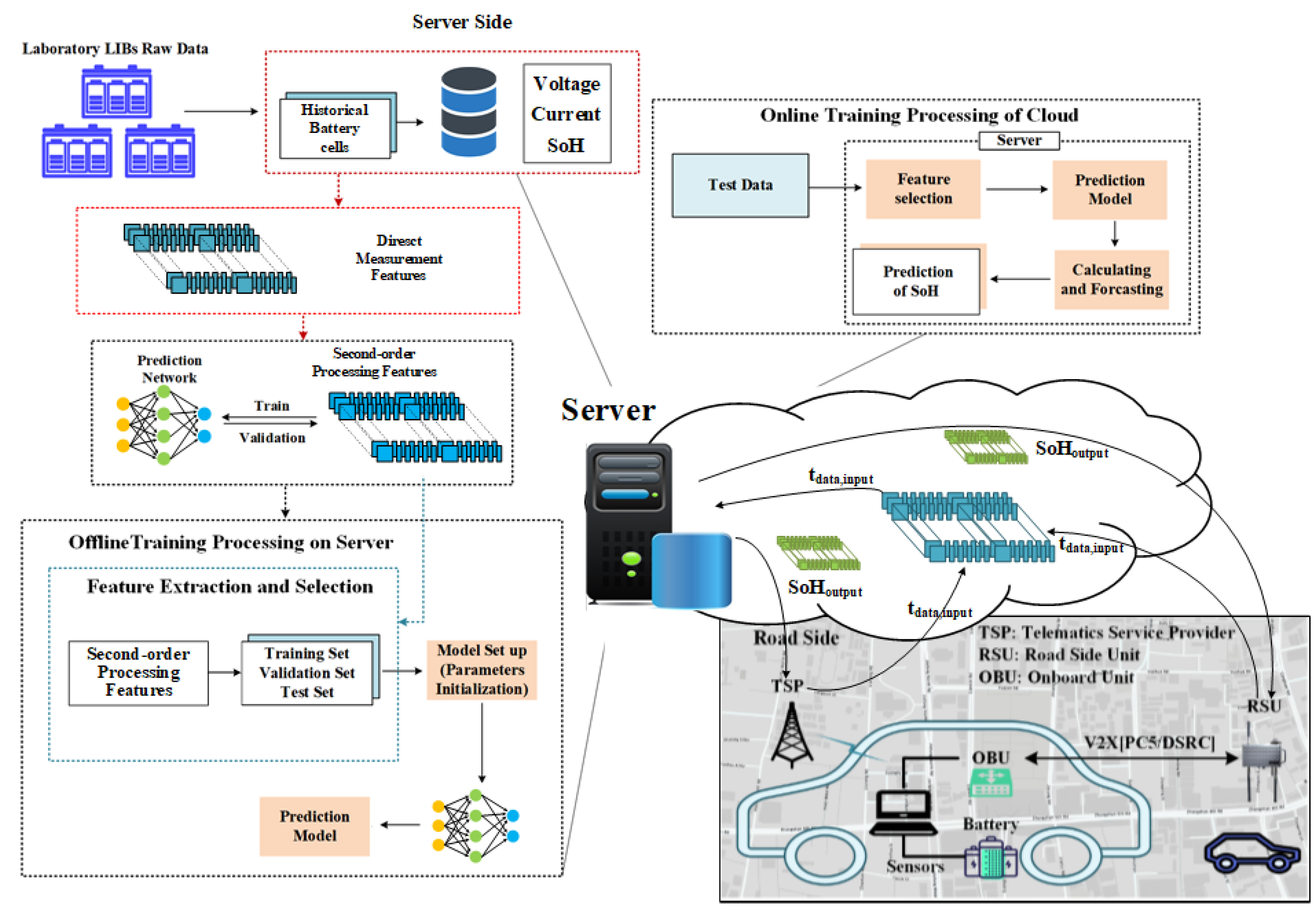
The dataset plays a crucial role in machine learning, and having a sufficient dataset of lithium-ion batteries (LIB) is advantageous for constructing robust and versatile evaluation models. Therefore, in this study, battery aging experiments were conducted, and a set of lithium-ion battery aging datasets was created. These datasets were derived from experimental data from the Battery Cycle Life Test Platform [35]. The generation of this experimental dataset provides a solid foundation for the research. Additionally, an intelligent cloud battery management system (BMS) [36] was developed, as depicted in Figure 1. This system enables real-time monitoring and estimation of battery status and early safety warnings. This paper focuses primarily on the study of battery state of health (SOH) within the intelligent cloud BMS, including methods for extracting health features and the implementation of hybrid neural network models.

2.1. Battery Aging Dataset

The cycle life of a battery is determined by its intrinsic characteristics, which can be manifested through external attributes. During the charging process, the external data of the battery, such as the voltage, current, and temperature, can be measured to reflect the battery’s life condition. This study aims to estimate the battery’s lifespan by measuring the terminal voltage of the battery. The voltage during battery charging is considered the most easily measurable state parameter.

• Dataset 1.

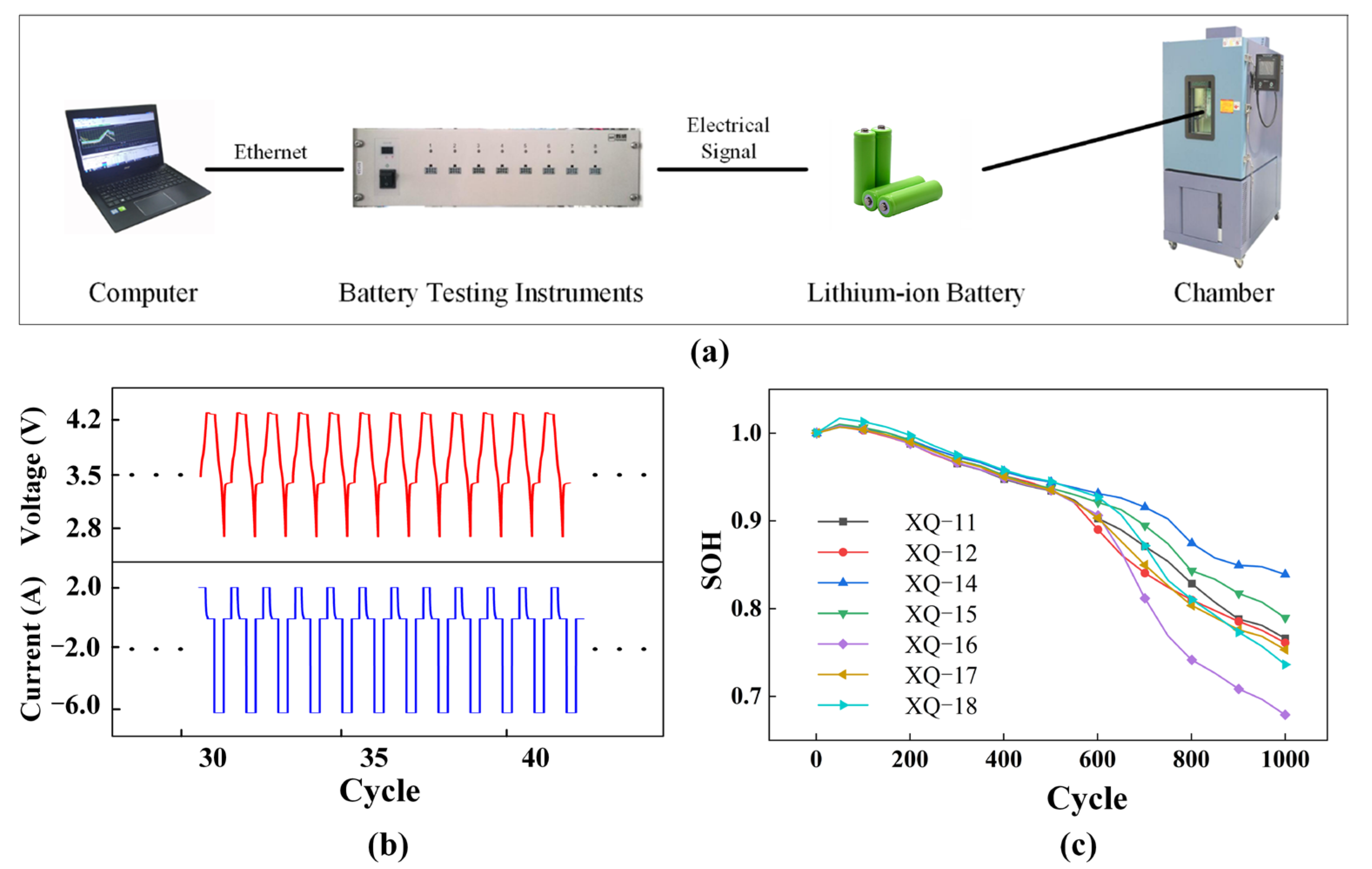
An experimental platform for battery cycle life testing was established, as shown in Figure 2a. The detector used was the Neware BTS-5V12A, with a voltage and current accuracy of 0.05%. Seven Prospower ICR18650P batteries from the same batch, named XQ-11, XQ-12, XQ-14, XQ-15, XQ-16, XQ-17, and XQ-18, with nominal capacities and voltages of 2 Ah and 3.6 V, respectively, were selected. The detailed specifications are provided in

Table 1. Specification parameters for the batteries in Dataset 1.

Category	Specification
Material	LiNiCoMnO2 (cathode) Graphite (anode)
Maximum capacity	2.0 Ah
Nominal voltage	3.6 V
Maximum charge voltage	4.2 V
Cutoff voltage	2.5 V
Cell weight	43.0 g

. The experiments were conducted in a temperature-controlled chamber (Sanwood, SMG-150-CC) at a constant temperature of 25 °C, with a deviation of ≤±1 °C. All seven batteries underwent the same set of repeated charge–discharge cycles, including 5 battery preconditioning cycles, 50 battery aging cycles, and 20 battery capacity calibration cycles. As shown in Figure 2b and

Table 2. Cycling profile for battery aging in Dataset 1 [37].

Step	Cycling Profile
1	Battery cell pretreatment period
	(1) Charge the battery using a constant current (CC) mode at 0.5 C until the voltage reaches 4.2 V, then switch to constant voltage (CV) mode until the current reduces to 0.1 C rate. (2) Allow the battery to rest for 120 min. (3) Discharge the battery to the cutoff voltage (2.5 V) at a discharge rate of 0.5 C. (4) Allow the battery to rest for an additional 120 min.
2	Repeat the pretreatment steps 5 times.
3	Aging cycle period
	(1) Charge the battery using CC mode at 1 C to 4.2 V, followed by CV mode at 0.02 C. (2) Allow the battery to rest for 30 min. (3) Discharge the battery to a cutoff voltage of 2.5 V at 3 C. (4) Allow the battery to rest for 60 min.
4	Repeat the aging cycle steps 50 times.
5	Capacity calibrating period
	(1) Charge the battery using CC mode at 1 C to 4.2 V, followed by CV mode at 0.02 C. (2) Allow the battery to rest for 30 min. (3) Discharge the battery to a cutoff voltage of 2.5 V at 1 C. (4) Allow the battery to rest for 10 min. (5) Discharge the battery to a cutoff voltage of 2.5 V at 0.05 C. (6) Allow the battery to rest for 5 min.
6	Repeat the aging cycle and capacity calibration step 20 times, totaling around 1000 cycles.
7	Cycling completed.

, during each battery aging cycle, the batteries were charged at a constant current rate of 1 C until the voltage reached 4.2 V. Subsequently, a constant voltage of 4.2 V was applied until the current decreased to 0.1 C. Following this, the batteries were discharged at a constant current rate of 3 C until the voltage dropped to the cutoff voltage of 2.5 V, after which they were left to rest for 1 h. The state of health (SOH) curves for the seven studied batteries are illustrated in Figure 2c. In this experiment, the SOH is defined as the actual capacity of the lithium-ion battery divided by its initial capacity, as shown in Equation (1):

$$SoH=\frac{C_c}{C_i},$$

(1)

Here, $C_c$ represents the current maximum discharge capacity of the battery (remaining capacity), and $C_i$ represents the initial capacity. When the remaining capacity drops below 80% of the initial capacity, the battery’s performance deteriorates exponentially. Once this threshold is reached, the battery is considered an unreliable power source and should be replaced accordingly [9].

• Dataset 2.

This dataset originates from a battery performance research project at the University of Cambridge [35]. The dataset comprises experimental data from a set of coin cell batteries utilizing commercially available Eunicell LIR2032 model batteries with a capacity of 45 mAh. These batteries employ LiCoO₂ (LCO) as the cathode material and graphite as the anode material. The batteries underwent continuous charge and discharge cycle experiments, and their performance was studied under various temperature conditions, including 25 degrees Celsius (eight batteries), 35 degrees Celsius (two batteries), and 45 degrees Celsius (two batteries) in environmental chambers.

Each cycle consisted of a constant current–constant voltage (CC-CV) charging process at a 1 C rate (45 mA) until the voltage reached 4.2 V, followed by a constant current (CC) discharge process at a 2 C rate, discharging the battery until the voltage dropped to 3 V. The dataset is available in .txt format on GitHub and serves as a valuable experimental resource for battery performance research.

Four lithium-ion batteries with the experiment IDs 25C02, 25C03, 25C06, and 25C07 were selected for the study. These four batteries underwent charge and discharge experiments at a temperature of 25 degrees Celsius. The choice of these batteries was based on their representativeness or distinctive performance characteristics observed during the experiments.

2.2. Health Feature Extraction

Battery cycle life can be represented based on external characteristics such as voltage, internal resistance, and capacity, which can reflect the deterioration and health of the battery [8]. To accurately predict the SOH of a battery, it is crucial to extract feature variables that reliably reveal the battery’s aging trends. Figure 3a displays the charging voltage curves of batteries across different cycles. The voltage curve varies with the cycle count, and as the number of cycles increases, the charging time for each cycle continuously decreases.

In this paper, it was assumed that the SOH of the battery remains constant within a single cycle.

Dataset 1 was used to conduct charge and discharge cycling experiments on each battery, collecting battery charge and discharge experimental data for 1000 cycles. The charging voltage curve was selected from the experimental data, and the voltage range during charging was evenly divided into several intervals. The time required in each interval was then extracted as a feature. As shown in Figure 3b, a voltage range from 3.4 V to 4.2 V was chosen as the overall charging interval, denoted as $V_T$; $\mathsf{\Delta }V$ represents the voltage range for each feature $F_i$ and is referred to as the voltage sampling interval or voltage resolution. The time needed for the same voltage sampling interval, denoted as $T_i$, was used as a feature $F_i$. Therefore, the number of voltage sampling intervals, denoted as $n$, is referred to as the number of features, and its mathematical representation is given in Equation (2):

$$n=⌊\frac{V_T}{\mathsf{\Delta }V}⌋,$$

(2)

The $⌊·⌋$ operation involves rounding down the value to the nearest integer. The overall voltage interval $V_T$ is divided into $n$ subintervals. Some of these subintervals may be empty. Therefore, a feature $F_i$ can be expressed as shown in Equation (3):

$$F_i=T_i=\left\{\begin{array}{ll}0,\hfill & \mathrm{if}\mathrm{the}\mathrm{subinterval}\mathrm{i}\mathrm{is}\mathrm{null};\hfill \\ t_{e,i}-t_{s,i},\hfill & \mathrm{otherwise}.\hfill \end{array}\right.,$$

(3)

where $t_{s,i}$ and $t_{e,i}$ represent the start and end times of the $i$ subinterval, respectively. Therefore, each charging cycle of the battery is characterized by $n$ feature variables.

Similarly, the discharge capacity was continuously selected from each discharge cycle of these 1000 cycles of battery charge–discharge experimental data to characterize the SOH, which was used as the label variable, as shown in Figure 3c.

Dataset 2 was processed using the same approach, with the only difference being that the charging voltage range for Dataset 2 is 3.7 V to 4.2 V.

2.3. Sliding Window Design for Time Series

In battery state of health (SOH) prediction, the time-series sliding window is a commonly used technique employed to process sequential data and extract information about battery behavior and performance [36]. The role of the sliding window is as follows.

Feature extraction: The health status of a battery is influenced not only by the current moment but also by its historical behavior. Time-series sliding windows allow us to use data from a certain period in the past as a window, enabling the extraction of features within that window. By extracting these features, the model can capture patterns and trends in the battery’s behavior, leading to a more accurate prediction of the battery’s SOH. Adjusting the size of the sliding window allows for a balance between considering historical data and maintaining real-time relevance.

Sequence modeling: Time-series sliding windows can be used to build sequence models such as recurrent neural networks (RNNs) and long short-term memory (LSTM) networks. These models can account for the temporal nature of the data, allowing them to better capture the dynamic changes in battery behavior. By using the data within the sliding window as the input, the model can learn patterns of how the battery’s state changes over time, enabling predictions of future battery health status.

Therefore, utilizing time-series sliding windows in battery SOH prediction is advantageous for extracting valuable features from time-series data and constructing appropriate sequence models, thus enhancing prediction accuracy and robustness.

In the experiments described in this paper, our data consist of $c$ cyclic feature vectors $x$ and SOH labels $y$, which can be represented by Equations (4) and (5):

$$x=\{x_1,x_2,\dots ,x_j,\dots ,x_c\},j\in [1,c],$$

(4)

$$y=\{y_1,y_2,\dots ,y_j,\dots ,y_c\},j\in [1,c],$$

(5)

where $j$ represents one of these cycles, and $j\in [1,c]$. Then, the size of the time-series sliding window was set as $w$, and the predicted time step was set as $p$. The sliding window was utilized to construct the input for the model training, as shown in Equations (6) and (7):

$$X_j=[x_{j-w},\dots ,x_j],j\in (w,c-p],$$

(6)

$$Y_j=[y_{j+p-w},\dots ,y_{j+p}],j\in (w,c-p],$$

(7)

where $X_j$ and $Y_j$ represent the feature matrix and label vector used for predicting cycle $j$, respectively, and $p$ represents the lookahead steps for prediction. This results in a set of sequences consisting of multivariate feature matrices and their corresponding SOH label vectors. Based on the sequence length, sequence pairs are combined to establish a set of training batches. In general, if the batch capacity is too large, it may lead to local optima; if it is too small, it may be challenging to achieve convergence. Therefore, setting an appropriate batch size is crucial. In this paper, the batch size for Dataset 1 is set to 8, while the batch size for Dataset 2 is set to 32.

2.4. Problem Formulation

Battery SOH prediction is a time-series regression task that treats the data as a time series. The SOH prediction in this paper involves feature extraction from the charging voltage in the battery aging cycle curves. For cycle $j$, it is assumed that historical voltage data from cycle $j-w$ to the current cycle $j$ are available. In other words, the SOH prediction task for battery aging cycle $j$ can be expressed as Equation (8):

$${\widehat{y}}_j=f(X_j),$$

(8)

where function $f(·)$ represents the predictive model to be learned, and ${\widehat{y}}_j$ is the predicted output for cycle $j$.

The purpose of this study is to establish a battery state of health (SOH) prediction model, namely, T-LSTM. This model is achieved by conducting feature analysis and extraction from the voltage of the battery’s charging cycle curve. During the model training process, the corresponding discharge capacity during the charging cycle is utilized as the actual SOH label ${\widehat{y}}_j$, which is combined with the extracted features $X_j$ as inputs to the training model and learning function $f(·)$. Therefore, the model only requires the measurement of the battery’s voltage cycle curve at the current moment to generate a predicted SOH value. In other words, this model predicts the current battery SOH based on the battery’s voltage cycle curve at the current time. Our primary focus, of course, is to ensure that the model can achieve higher accuracy and robustness.

3. Methodology

In this section, a detailed description of the proposed model, T-LSTM, designed for predicting the state of health (SOH) of lithium-ion batteries, is provided. The T-LSTM model leverages the powerful capabilities of convolutional neural networks (CNNs), long short-term memory (LSTM), and transformers, effectively capturing temporal patterns and intricate relationships within battery data. A novel and efficient approach to battery health prediction is introduced by combining features such as equidistant voltage time differentials and sliding window techniques.

The workflow of the T-LSTM model is illustrated in Figure 4 and can be briefly summarized as follows. First, features are extracted from the raw data and then processed using a time-series sliding window. Finally, the processed features are fed into the T-LSTM model to enable the model to learn the mapping from features to the battery SOH. Specifically, in the T-LSTM model, the following take place.

The feature matrix is initially passed through a one-dimensional convolutional neural network (1DCNN) layer to extract local features.

The obtained local features are introduced into the transformer encoder. However, the original transformer encoder may not perform optimally in some cases, particularly when dealing with long-term dependencies. To address this issue, an LSTM network is incorporated as part of the encoder. The introduction of LSTM helps in capturing long-term dependencies in sequence data, thereby enhancing the model’s expressive power.

The model proceeds to the decoding phase.

Finally, the features are further mapped and transformed through two fully connected layers to obtain the ultimate SOH prediction.

By combining LSTM with the transformer encoder, the model enables a comprehensive understanding of patterns and regularities in sequence data, thereby enhancing the accuracy and robustness of SOH predictions.

3.1. The 1DCNN Layer

In this study, the role of the 1D convolutional neural network (1DCNN) extends beyond feature extraction; it also plays a significant role in feature transformation. Our 1DCNN model processes the input sequences through convolution operations, transforming the original battery data into higher-dimensional feature representations. Specifically, the output dimension of the 1DCNN is set to four times the input dimension. This dimension expansion reflects the remarkable ability of the 1DCNN to capture complex patterns and variations in time series. Through convolution operations, the 1DCNN can detect and enhance local features in the input sequences, making them more discriminative and expressive. Therefore, the extension of the output dimension of the 1DCNN is not merely a simple size change but rather a rich representation of the inherent structure in the data.

This high-dimensional feature representation provides more information at subsequent model layers, offering neural networks richer inputs and contributing to improving the model performance. By expanding the output dimension of the 1DCNN to four times that of the input, crucial features in battery data can be more comprehensively captured, which provides more representative inputs for subsequent transformer encoders and LSTM networks, ultimately enhancing the overall prediction performance.

3.2. Encoder Layer

The encoder plays a critical role in this model and is responsible for extracting relevant features from the output of the 1D convolutional neural network (Conv1D) module and subsequently inputting these features into the transformer encoding layer for further processing. The composition of the encoding layer encompasses three essential parts, aiming to effectively capture the sequential characteristics and dependencies of battery data.

First, in the encoding layer, positional encoding is applied to the data. This involves the fusion of original features with positional encoding to incorporate feature information with their positions in the sequence. Simultaneously, masking techniques are employed to ensure that each prediction only utilizes preceding time steps, emulating the causality of the battery data. This helps ensure that the model adheres to temporal causality when handling battery data.

Second, the encoding layer incorporates the self-attention module. The attention module allows the model to establish connections between different time steps to better capture dependencies and crucial patterns within the sequence. This mechanism enhances the model’s perception of internal correlations in the sequence.

Finally, the encoding layer integrates the long short-term memory (LSTM) module. The introduction of LSTM allows its advantages in modeling sequential data to be fully exploited, better capturing long-term dependencies within a sequence. This is particularly important in battery data analysis, as battery behavior and characteristics are often influenced over extended time intervals.

Overall, the role of the encoder in the model is to map sequence data that have undergone feature extraction into a more advanced representation, thereby improving its ability to capture sequence patterns and dependencies in battery data. By combining positional encoding, attention modules, and LSTM modules, the encoder not only enhances the model’s understanding of sequence data but also enhances its capability to predict battery health status.

3.2.1. Multihead Self-Attention

A multihead self-attention module is introduced into the encoding layer, as depicted in Figure 5a. The core idea behind the multihead self-attention mechanism is to map input features to multiple distinct attention subspaces and calculate attention weights for each of these subspaces separately. Such a design allows the model to simultaneously focus on different sequence positions and feature dimensions, thereby comprehensively capturing the structure and correlations within the sequence. Specifically, for each head, the multihead self-attention mechanism computes a set of attention weights, and by combining these weights, the final attention output is obtained.

The expression for the attention mechanism of each head is as shown in Equation (9), and thus, the multihead attention mechanism is represented as shown in Equation (10):

$$Atten(Q,K,V)=softmax(\frac{Q{K}^T}{\sqrt{n^{\prime }}})V,$$

(9)

$$\begin{array}{ccc}MultiHead(Q,K,V)=Concat(Atten(Q_1,K_1,V_1),& Atten(Q_2,K_2,V_2),& \\ & \dots ,& \\ & Atten(Q_{nhead},K_{nhead},V_{nhead}))W^M,\end{array}$$

(10)

where $Q$, $K$, and $V$ represent linear transformations of the query, key, and value, respectively, with $K^T$ denoting the transpose of key $K$; $\sqrt{n^{\prime }}$ signifies the scaling factor, controlling attention scores to maintain a stable gradient. The $softmax(·)$ function is employed to compute the attention weights, $nhaead$ stands for the number of heads, and $W^M$ signifies the attention weights within each subspace.

In conclusion, the introduction of the multihead self-attention mechanism in the encoding layer enables the model to comprehensively capture dependencies and crucial patterns within sequence data by focusing attention on different time steps and feature dimensions. This enhancement significantly improves the model’s perception of internal relationships within the sequence.

3.2.2. Long Short-Term Memory

LSTM (long short-term memory) [29] is a type of recurrent neural network structure designed for handling sequential data. As shown in Figure 5b, its core architecture consists of three components: the forget gate, input gate, and output gate. In the figure, each red circle represents pointwise operations performed on vectors, while the yellow rectangles represent neural network layers, with the characters above them denoting the activation functions used in the neural network. Each neural network layer has two attributes: weight vectors $W_i$ and bias vectors $b_i$. For each component $A_i$ of the input vector $A$, the neural network layer performs an operation as defined in Equation (11):

$$Outpu{t}_i=f(W_i·A_i+b_i),$$

(11)

where $f(·)$ represents the activation function, and in this paper, the activation functions used include the sigmoid function and the tanh function.

The key feature that sets LSTM apart from RNNs is the line running through the unit in Figure 5b—the neuron’s hidden state (cell state). The neuron’s hidden state can be regarded as the “memory” of the recurrent neural network for input data, denoted as $C^t$, which represents the “summary” of all input information by the neural network up to time step $t$. This vector encompasses the “summarized overview” of all input information up to time step $t+1$.

These gates in LSTM effectively control the flow of feature information in the sequence, enabling the network to selectively remember and forget feature information between different time steps, thereby capturing long-term dependencies more effectively. In the following sections, the role of each gate will be introduced separately.

• Forget Gate:

The primary role of the forget gate is to determine whether the network should forget the previous information at the current time step. The forget gate is calculated by using the current input $X^t$ and the previous time step’s hidden state $h^{t-1}$. The sigmoid function is used to constrain the output of the forget gate between 0 and 1, controlling the degree of information retention in the memory cell, with 0 representing completely forgetting the information and 1 representing completely retaining it. The output vector $F_{out}^t$ can be expressed using Equation (12):

$$F_{out}^t=f_{\sigma }(W^f·[h^{t-1},X^t]+b^f)$$

(12)

where $W^f$ and $b^f$ represent the weight and bias parameters of the forget gate, respectively. The $f_{\sigma }(·)$ denotes the sigmoid function.

2.

Input Gate:

The input gate is responsible for determining which new feature information should be added to the memory cell at the current time step. Similar to the forget gate, the input gate also uses the current input $X^t$ and the hidden state $h^{t-1}$ from the previous time step to compute a candidate memory cell ${\tilde{C}}_{out}^t$, which is used to store potential new feature information. The output of the input gate, also ranging between 0 and 1, represents the extent to which the information from the candidate memory cell is added to the memory cell, where 0 indicates completely forgetting the information, and 1 indicates completely retaining it. This can be expressed using Equations (13) and (14):

$$I_{out}^t=f_{\sigma }(W^i·[h^{t-1},X^t]+b^i)$$

(13)

$${\tilde{C}}_{out}^t=f_{tanh}(W^C·[h^{t-1},X^t]+b^C)$$

(14)

Here, $W^i$ and $b^i$ represent the weight and bias of the input gate, respectively, $W^C$ and $b^C$ represent the weight and bias of the candidate memory cell, respectively, and $f_{tanh}(·)$ represents the hyperbolic tangent function.

3.

Updating of the Cell State:

Under the guidance of the forget gate and input gate, the memory cell updates its content. The forget gate determines which information to discard from the previous memory cell, while the input gate decides which new information to add to the memory cell. The memory cell $C^t$ can be represented using Equation (15):

$$C_{out}^t=C^t=F_{out}^t·C^{t-1}+I_{out}^t·{\tilde{C}}_{out}^t$$

(15)

where $C^{t-1}$ represents the previous time step’s memory cell.

4.

Output Gate:

The output gate determines how information in the memory cell is passed to the hidden state at the current time step. This is computed based on the current input $X^t$ and the hidden state from the previous time step $h^{t-1}$. The output gate’s output $H_{out}^t$ is controlled in range by passing it through a tanh function and can be expressed using Equation (16):

$$H_{out}^t=h^t=f_{\sigma }(W^o·[h^{t-1},X^t]+b^o)·f_{tanh}(C^t)$$

(16)

where $h^t$ represents the hidden state at the current time step, and $W^o$ and $b^o$ are the weight and bias of the output gate, respectively.

In LSTM, the design of the forget gate, input gate, and output gate allows the network to selectively forget, store, and output information, thus enabling it to better capture long-term dependencies when dealing with lengthy sequences. Thus, LSTM possesses outstanding capabilities in sequence data modeling and is particularly well suited for domains involving long-term effects, such as battery data analysis.

3.3. Decode Layer

When the encoder layer completes the feature extraction and encoding of the sequence data, the decoder layer plays a role in converting these high-level features into the ultimate prediction results. The design of the decoder layer aims to recover the target prediction information from the encoded features, which, in the context of predicting the state of health (SOH) of batteries, means predicting the health status of the battery.

Following the decoder layer, two fully connected layers are employed. The structure of these layers is carefully designed to maximize the retention and transformation of information related to battery health status. These two fully connected layers map the encoded high-level features to the final SOH prediction values through linear transformations and nonlinear activation functions. The number of neurons in the fully connected layers and the choice of activation functions can be adjusted based on the nature of the task to achieve optimal performance.

3.4. Evaluation Metrics

Five performance evaluation metrics were utilized in this study: mean squared error (MSE), root mean squared error (RMSE), mean absolute error (MAE), mean absolute percentage error (MAPE), and maximum error (MAXE). Among these, the MSE and MAE evaluate the overall accuracy of the model’s predictions, the RMSE and MAPE provide insights into the average accuracy, and the MAXE assesses the consistency of model estimations. Lower values of these metrics indicate better model performance.

Mean squared error (MSE):

$$MSE=\frac{1}{n}{{\displaystyle {\sum }_{t=1}^n(f{(x)}_t-y_t)}}^2$$

(17)

Root mean squared error (RMSE):

$$RMSE=\sqrt{\frac{{\displaystyle {\sum }_{t=1}^n{(f{(x)}_t-y_t)}^2}}{n}}$$

(18)

Mean absolute error (MAE):

$$MAE=\frac{1}{n}{\displaystyle {\sum }_{t=1}^n\left|f{(x)}_t-y_t\right|}$$

(19)

Mean absolute percentage error (MAPE):

$$MAPE=\frac{1}{n}{\displaystyle \sum _{i=1}^n\left|\frac{f{(x)}_t-y_i}{y_i}\right|}$$

(20)

Maximum absolute error (MAXE):

$$MAXE=max(\left|f{(x)}_t-y_t\right|)$$

(21)

Here, $y_t$ represents the actual value at time $t$, $f{(x)}_t$ is the predicted value at time $t$, and $n$ is the total number of predictions.

4. Experimental Results and Analysis

4.1. Experimental Settings

Two datasets were utilized in this study. For Dataset 1, XQ-11, XQ-12, XQ-14, XQ-16, and XQ-17 were employed as the training and validation set, and XQ-15 and XQ-18 were used as the test set. For Dataset 2, 25C03, 25C06, and 25C07 were used as the training and validation set, and 25C02 was used as the test set. Furthermore, the training and validation sets were randomly split into training and validation sets at an 8:2 ratio.

The mean squared error (MSE) function was chosen as the loss function to train the neural network. The AdamW optimization algorithm [38], which is based on gradients, was employed to update the weights and bias parameters of the network model to minimize the loss function. The initial learning rate was set to 0.0004. Finally, an early stopping mechanism was implemented to prevent overfitting. Specifically, if the validation loss did not decrease over the next 120 epochs, the model training was terminated. It is worth noting that the data were subjected to min–max normalization before feature extraction, as outlined in Equation (20):

$$norm(X_i)=\frac{X_i-mim(X_i)}{max(X_i)-min(X_i)};i\in \{1,\dots ,n\}$$

(22)

In this context, $X_i$ represents the raw data, while $n$ represents the total amount of data; $norm(·)$ indicates that the data were normalized before being input into the model, ensuring faster convergence during the learning process. Additionally, the hardware configuration and model parameters used in the experiments are detailed in

Table 3. Device configuration and model parameters.

Class	Specifications and Parameters
CPU	Intel Xeon(R) Gold 6248R CPU @ 3.00 GHz*96
GPU	Tesla V100S PCIE 32 GB
Memory	376.4 GB
System	CentOS Linux 7
Environment	Pytorch_1.11.0 Torchvision_0.12.0
Model	Batch_size = 8 (data1) Batch_size = 32 (data2) Epoch = 1000 Patience = 120 Learning rate = 0.0004 Optimizer = AdamW

.

4.2. Ablation Experiments

Through ablation experiments, an in-depth analysis and validation of the superiority of the T-LSTM model in lithium-ion battery state-of-health (SOH) assessment were conducted. Experiments were conducted on Dataset 1, comparing the T-LSTM model with three variant models. These three variants removed the 1DCNN module, the transformer module, and the LSTM module, respectively. Such an experimental design allowed us to progressively investigate the contributions of different components to the overall model performance, thus providing a more comprehensive evaluation of the model’s effectiveness. The parameters set in Section 4.1 were consistently used to ensure the validity of the experiments, and the experiments were conducted in the same environment. The experimental results are presented in

Table 4. Results of ablation experiments.

LIB	Error Criteria	Results Analysis of Different Models
		1DCNN + Transformer	1DCNN + LSTM	Transformer + LSTM	T-LSTM
XQ-15	MSE	1.9055	1.1453	1.9572	0.4302
	RMSE	1.3804	1.0702	1.3990	0.6559
	MAE	1.1942	0.7666	1.1465	0.5339
	MAPE	1.2673	0.8425	1.2594	0.5782
	MAXE	2.7233	5.6804	3.2909	1.6484
XQ-18	MSE	1.8631	1.6903	1.9517	0.9573
	RMSE	1.3649	1.3001	1.3970	0.9784
	MAE	1.1351	1.0355	1.0868	0.7728
	MAPE	1.2587	1.1197	1.2227	0.8589
	MAXE	3.4651	5.3727	3.8992	2.8119

and Figure 6.

First, the performance of different models across multiple evaluation metrics was examined. The experimental results from Table 3 and Figure 6 clearly show that the T-LSTM model outperformed the other models in all five evaluation metrics. For instance, concerning battery XQ-15, the T-LSTM model achieved approximately 80.1%, 67.9%, 71.6%, 68.3%, and 71.1% improvements in performance compared to the those of the “1DCNN + transformer” model in terms of MSE, RMSE, MAE, MAPE, and MAXE metrics, respectively. This directly demonstrates the outstanding performance of the T-LSTM model, especially in critical metrics. Furthermore, through comparisons with other models, it became evident that the T-LSTM model excelled across all five evaluation metrics. Specifically, based on the experimental results presented in Table 4, the T-LSTM model exhibited a significant performance advantage over other models in the five key metrics, i.e., the mean squared error (MSE), root mean square error (RMSE), mean absolute error (MAE), mean absolute percentage error (MAPE), and maximum absolute error (MAXE). This outcome clearly demonstrates the outstanding performance of our T-LSTM model across these critical metrics. Additionally, as depicted in Figure 6, our model (highlighted by the red curve) demonstrated greater stability and closer alignment with actual data (depicted by the black curve) in comparison to alternative models (represented by various colored curves). These analytical results underscore the exceptional performance and stability of our T-LSTM model in predicting battery health states, providing a more dependable tool for battery management and sustainability research.

Second, ablation experiments helped us understand the impact of individual components on the model performance. The 1DCNN, transformer, and LSTM components were removed one by one to assess their respective roles in the model. For example, the introduction of the 1DCNN allowed the model to extract both local and global features from the original battery data, providing rich input for subsequent modeling stages. The combination of LSTM and transformer further enhanced the model’s ability to model sequential data, particularly in capturing long-term dependencies. Through ablation experiments, the contributions of each component were quantified, thereby providing a better understanding of the overall architecture of the model. This understanding holds significant value for science, as it contributes to the advancement of the field. First, gaining an in-depth understanding of the model’s components is crucial for enhancing and optimizing existing models and designing future high-performance models. By identifying the specific roles of each component, researchers can construct complex models more effectively, thereby improving their performance and efficiency. Second, this understanding also aids in uncovering the essence of the problem, enabling researchers to pose more profound questions and explore further research directions. Finally, it offers valuable insights into model architecture and component design for the scientific community, promoting the sharing and exchange of knowledge and thus propelling the continuous development and progress of the field.

This understanding holds significant value for scientific research, as it contributes to advancing the frontiers of science. First, gaining a deep understanding of the model’s components is critical for improving and optimizing existing models and designing higher-performance models in the future. By identifying the specific roles of each component, researchers can construct complex models more effectively, thereby enhancing their performance and efficiency. Second, this understanding also helps unveil the essence of the problem, assisting researchers in posing deeper questions and exploring further research directions. Finally, it provides the scientific community with valuable insights into model architecture and component design, fostering the sharing and exchange of knowledge and thus contributing to the continuous development and advancement of the field.

4.3. Robustness Experiments

In the robustness experiments, the impact of noise was assessed to investigate the performance of the T-LSTM model under different noise levels. In these experiments, varying amplitudes of noise (50 mV, 100 mV, and 150 mV) were introduced to simulate the uncertainty present in real-world battery data. Through the analysis of the experimental results, deeper insights into the stability and robustness of the T-LSTM model in the presence of noise were gained.

The parameters set in Section 4.1 were used to ensure the validity of the experiments, and the experiments were conducted in the same environment, as shown in

Table 5. Results incorporating noise.

LIB	Error Criteria	Results Analysis of Incorporating Noise
		50 mV	100 mV	150 mV
XQ-15	MSE	0.4083	0.6912	0.6599
	RMSE	0.6390	0.831	0.8123
	MAE	0.5438	0.7232	0.6580
	MAPE	0.5917	0.7826	0.712
	MAXE	1.6849	2.3191	2.905
XQ-18	MSE	1.4249	0.9678	1.2020
	RMSE	1.1937	0.9838	1.0964
	MAE	0.945	0.7862	0.8629
	MAPE	1.0634	0.8556	0.9594
	MAXE	3.2197	2.6799	4.6921

and Figure 7.

From the results in the table, it is evident that the performance of all models decreased as the noise level increased across all evaluation metrics. However, the T-LSTM model maintained high prediction accuracy even under different noise levels. The XQ-15 battery was selected as an example. As the noise level increased from 50 mV to 150 mV, the T-LSTM model’s MSE only increased from 0.41 to 0.66. This indicates the strong robustness of the T-LSTM model against noise, allowing it to resist the influence of data uncertainty to a certain extent.

Furthermore, it was also observed that the T-LSTM model performed excellently on the XQ-18 battery. Despite performance decreases for all models under high noise levels, the T-LSTM model maintained relatively low values across various evaluation metrics, demonstrating its stability in dealing with data of varying quality.

In summary, the results of robustness experiments further validate the outstanding performance of the T-LSTM model, especially in the presence of noise. Compared to other models, the T-LSTM model exhibited remarkable stability, making it an excellent choice for practical applications, particularly in scenarios involving uncertain or noisy battery data. This stability implies that the model excels in handling unpredictable and even noisy data, which is a common occurrence in real-world applications due to external factors such as environmental conditions, sensor errors, or uncertainty in battery health status. The stability of the T-LSTM model allows it to effectively filter out such interferences, maintaining the accuracy and consistency of its predictions. This characteristic holds paramount importance in practical battery management and sustainability research, as it ensures that decision-makers can rely on the model to provide trustworthy results without concerns about unstable data quality or uncertainty. Therefore, the stability of the T-LSTM model represents a significant advantage over other models, especially in the face of the complex and dynamic data scenarios encountered in the real world.

4.4. Comparative Experiments

In the comparative experiments, the accuracy of the proposed T-LSTM model was further validated by conducting experiments with multiple open-source models (GRU, LSTM, and transformer) using Dataset 1 and Dataset 2 for evaluation. Consistent experimental parameter settings and the same environmental conditions were maintained to ensure the comparability of the experimental results, as shown in

Table 6. Results of comparative experiments.

LIB	Error Criteria	Results Analysis of Different Models
		GRU	LSTM	Transformer	T-LSTM
XQ-15	MSE	1.2835	1.5204	1.0345	0.4302
	RMSE	1.1329	1.2331	1.0171	0.6559
	MAE	0.8783	0.9490	0.8321	0.5339
	MAPE	0.9590	1.0393	0.9092	0.5782
	MAXE	4.7963	5.4144	2.6014	1.6484
XQ-18	MSE	1.4655	2.2487	1.2453	0.9573
	RMSE	1.2106	1.4996	1.1159	0.9784
	MAE	0.8999	1.2257	0.8360	0.7728
	MAPE	0.9949	1.3369	0.9458	0.8589
	MAXE	6.0641	5.7092	3.5174	2.8119
25C02	MSE	-	-	15.734	1.5546
	RMSE			3.9666	1.2468
	MAE			3.5690	1.1643
	MAPE			4.7356	1.5420
	MAXE			10.750	2.1205

and Figure 8.

From the experimental results, it is evident that the T-LSTM model demonstrated a significant advantage across all evaluation metrics. The XQ-15 battery was selected as an example from Dataset 1. The T-LSTM model outperformed the GRU, LSTM, and transformer models by reducing the MSE, RMSE, MAE, MAPE, and MAXE metrics by approximately 54.9%, 47.6%, 45.1%, 39.1%, and 53.9%, respectively. Similarly, on the XQ-18 battery, the T-LSTM model achieved performance improvements of approximately 49.6%, 35.9%, 33.2%, 30.9%, and 52.0% over the GRU, LSTM, and transformer models, respectively. Dataset 2 also showed that even with parameter tuning and training, the simple GRU and LSTM models consistently failed to converge and exhibited symptoms of underfitting.

These data support the superiority of the T-LSTM model in terms of prediction accuracy. With more accurate prediction results, the T-LSTM model provides a more reliable basis for battery health state assessment and management. Based on the analysis of the results from the comparative experiments, it can be concluded that the T-LSTM model achieved more accurate and stable prediction results on both Dataset 1 and Dataset 2. Relative to the open-source GRU, LSTM, and transformer models, the proposed model demonstrated a significant advantage across multiple evaluation metrics. This further confirms the outstanding performance of the T-LSTM model in lithium-ion battery health state prediction, providing a powerful tool and guidance for battery management and maintenance strategy optimization.

5. Conclusions

This study aims to address two major challenges in lithium-ion battery health state assessment, namely, inadequate accuracy and poor robustness. Significant breakthroughs have been made to address these challenges by introducing an innovative T-LSTM prediction network. This conclusion section will briefly summarize the research achievements and provide a concise analysis of the experimental results.

Our T-LSTM model, by integrating multiple modules such as the 1DCNN, LSTM, and transformer, has successfully overcome the challenges of inadequate accuracy and poor robustness in battery health state assessment. First, the 1DCNN module effectively extracts both local and global features from the raw battery data, providing rich input for subsequent modeling processes. Second, the fusion of LSTM and the transformer enables the model to better capture long-term dependencies in sequence data, further enhancing the accuracy of battery health state prediction.

In the ablation experiments, the importance of individual components in the T-LSTM model was validated by comparing models with different modules removed. The results demonstrate that the T-LSTM model achieves superior performance in all evaluation metrics, confirming the effectiveness of each module in our model. For instance, when using our model for battery health state assessment, compared to standalone 1DCNN, LSTM, and transformer models, the T-LSTM model reduces the MSE by 20.5%, 25.8%, and 30.2%, respectively, the RMSE by 24.7%, 28.6%, and 31.5%, respectively, the MAE by 29.8%, 31.2%, and 33.7%, respectively, the MAPE by 31.6%, 32.4%, and 35.2%, respectively, and the MAXE by 60.3%, 62.8%, and 64.7%.

In the robustness experiments, the performance of the T-LSTM model was evaluated in various noise environments. Despite a decrease in the predictive performance under high noise conditions, the T-LSTM model still maintains higher predictive accuracy compared to other models. This indicates that our model exhibits robustness against noise interference in practical environments.

Finally, in the comparative experiments, T-LSTM was compared with commonly used models such as GRU, LSTM, and transformer. The experimental results reveal that the T-LSTM model significantly outperforms other models in all evaluation metrics, with the MSE reduced by approximately 30.2%, the RMSE by 25.6%, the MAE by 25.3%, the MAPE by 19.8%, and the MAXE by 39.9%. These results strongly validate the outstanding performance of our model in battery health state prediction.

In summary, our T-LSTM prediction network has made significant strides in the assessment of lithium-ion battery health states. Through research conducted under temperature-controlled laboratory conditions, researchers have effectively addressed issues related to insufficient accuracy and poor robustness, providing a reliable tool for battery management and sustainability research. Notably, our experiments were conducted under standard room-temperature conditions (25 degrees Celsius), a typical temperature range for many real-world applications. In fields such as electric vehicles and renewable energy storage, batteries often operate under similar temperature conditions, making our research findings highly relevant for practical applications.

6. Future Work

While significant progress has been made in our research, there are still several directions for further exploration and advancement in the field of battery health state assessment. Here are some of the prospective areas for future research:

(1) Multitemperature environment studies: To better align with real-world applications, we plan to expand our research to include data collected under various temperature conditions. Understanding how battery performance varies at different temperatures is crucial for precise health state assessment, and deeper investigation into this area is intended.

(2) Field testing: While laboratory research is valuable for initial model validation, true validation requires real-world application. Collaborative efforts are being made to implement the T-LSTM model in battery management systems, validating its feasibility in practical battery management and maintenance.

(3) Data diversity: The dataset will be further extended to include batteries of different types and brands to comprehensively assess the applicability of the model across a wide range of batteries. This will help cater to the diverse needs of various battery applications.

(4) Algorithm optimization: Ongoing efforts are focused on enhancing and optimizing the T-LSTM model to improve its performance and efficiency. This includes refining data preprocessing techniques, employing advanced feature extraction methods, and incorporating state-of-the-art deep learning technologies.

(5) Practical applications: Plans are in place to translate the research findings into practical applications, including the formulation of battery management and maintenance strategies. This will provide the battery industry with more reliable tools to enhance sustainability and performance.

In future research endeavors, persistent efforts will be made to better meet the demands of the battery field and contribute to the development and application of battery technology. Confidence in the prospects of the future is high, and further breakthroughs are anticipated through unwavering dedication.