Abstract
The lithium-ion battery state of health (SOH) estimation is critical for maintaining reliable and safe working conditions for electric vehicles (EVs). However, accurate and robust SOH estimation remains a significant challenge. This paper proposes a multi-feature extraction strategy and particle swarm optimization-nonlinear autoregressive with exogenous input neural network (PSO-NARXNN) for accurate and robust SOH estimation. First, eight health features (HFs) are extracted from partial voltage, capacity, differential temperature (DT), and incremental capacity (IC) curves. Then, qualitative and quantitative analyses are used to evaluate the selected HFs. Second, the PSO algorithm is adopted to optimize the hyperparameters of NARXNN, including input delays, feedback delays, and the number of hidden neurons. Third, to verify the effectiveness of the multi-feature extraction strategy, the SOH estimators based on a single feature and fusion feature are comprehensively compared. To verify the effectiveness of the proposed PSO-NARXNN, a simple three-layer backpropagation neural network (BPNN) and a conventional NARXNN are built for comparison based on the Oxford aging dataset. The experimental results demonstrate that the proposed method has higher accuracy and stronger robustness for SOH estimation, where the average mean absolute error (MAE) and root mean square error (RMSE) are 0.47% and 0.56%, respectively.
1. Introduction
Vehicle electrification has been proven to be one of the most promising directions to reduce carbon dioxide emissions and solve the energy crisis. With the advantages of high power and energy density, high energy efficiency, and relatively long cycles of life, Lithium-ion batteries (LiBs) have become the primary power source of electric vehicles (EVs) [1]. However, during long-term cycling or storage, it is inevitable for LiBs to degrade, resulting in performance degradation or safety problems. Therefore, an accurate estimation of the state of health (SOH) is essential for the energy management system to maintain safe and high-efficient working conditions for EVs. Generally, the degradation of LiBs is an integrated consequence of internal and external factors. The internal factors mainly include the loss of active material (LAM), the loss of lithium inventory (LLI), resistance increase (RI), and solid electrolyte interface (SEI) growth [2,3]. Moreover, the external factors include operating temperature, charge and discharge rate, discharge depth, and cut-off voltage [4]. From the perspective of onboard applications, the loss of capacity and the increase of internal resistance are two widely used indicators to reflect the battery SOH, expressed as follows:
where and represent the capacity-based SOH and resistance-based SOH, respectively; and are the actual and nominal capacity, respectively; denotes the current resistance, and and are resistances of the end-of-life (EOL) and new battery, respectively. Compared to resistance-based SOH estimation methods, capacity-based SOH estimation methods draw more attention because capacity directly decides the driving range for EVs [5].
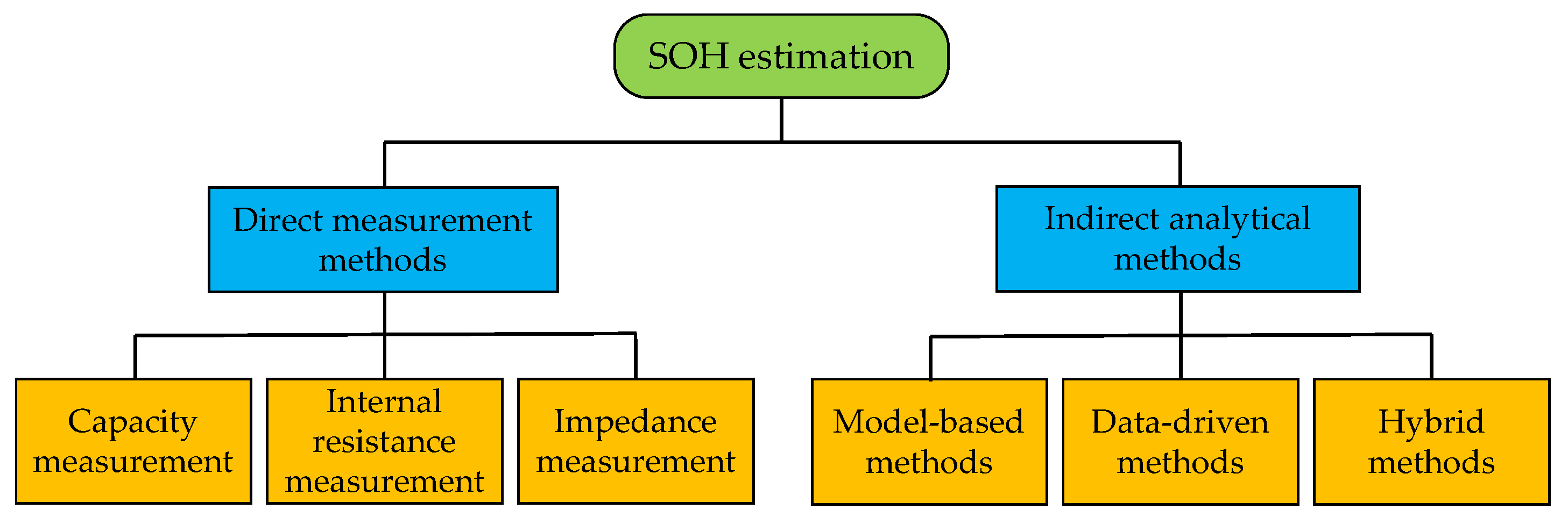
Generally, the existing SOH estimation methods can be divided into two categories, as shown in Figure 1 [6]: the direct measurement methods, like the capacity measurement method, internal resistance measurement test, and impedance measurement method, are suitable for laboratory condition but not practical in actual operations. Indirect analytical methods mainly include model-based, data-driven, and hybrid methods. According to the modeling mechanism, the model-based method can be divided into equivalent circuit model (ECM)-based method and electrochemical model (EM)-based method. The ECM employs lumped components, such as resistors, capacitors, and voltage sources, to describe the battery’s dynamic behavior [7]. It is one of the most promising approaches for online battery parameter identification and state estimation, owing to its ease of implementation and acceptable accuracy for EV applications. Based on the principle of ECM, a state equation and an observe equation are established. Then, filter-based methods, such as extended Kalman filter (EKF) [8] and unscented Kalam filter (UKF) [9], are used for online SOH prediction. The EM aims to describe the thermodynamics, Li-ion diffusion process, SEI film thickness, and side reaction kinetics inside the battery to realize the most accurate battery modeling and state estimation theoretically. However, with many parameters to be identified and partial differential equations, the onboard application of the EM-based SOH estimation remains a significant challenge. The trade-off between model complexity and accuracy still needs further research.

Figure 1.
Classification of SOH estimation methods.
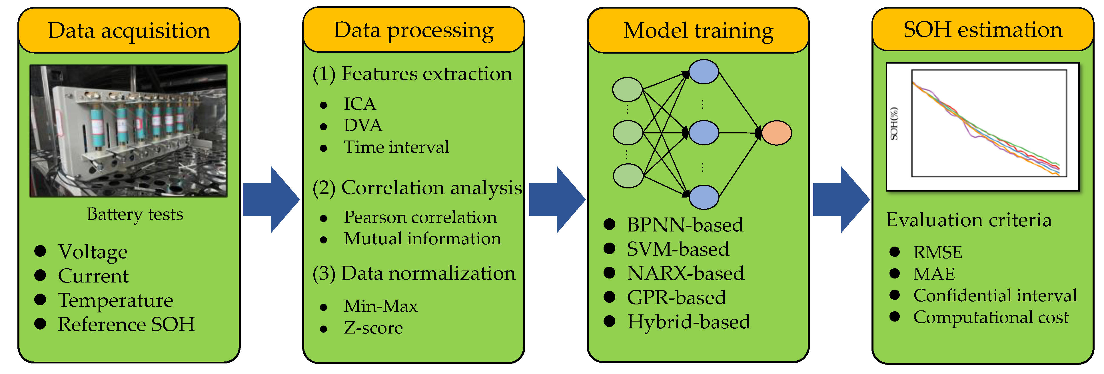
With the development of artificial intelligence, the machine learning (ML)-based data-driven method has gradually become the most popular method for SOH estimation [10]. The data-driven method can estimate battery states based on measured data. It does not require pre-knowledge about the battery aging mechanism or the battery models mentioned above, making it suitable and easily implementable for different LiBs. Typical procedures for developing data-driven SOH estimation methods are shown in Figure 2. In short, the first step is to conduct battery aging tests and collect raw data, such as voltage, current, and temperature. Since the raw data cannot provide sufficient information to reflect SOH, it cannot guarantee an accurate and robust SOH estimation either. The second step is hence to extract high-related health features (HFs) from the raw data using different techniques, such as model-based analysis, incremental curve analysis (ICA), and differential voltage analysis (DVA). In addition, correlation analysis is applied to analyze the correlation of the HFs. After that, the HFs and the reference SOH constitute the training dataset. Subsequently, different ML methods are used to learn and validate the nonlinear relationship between the input features and output based on the training dataset. Finally, the established ML algorithms can be used to estimate SOH for new data.
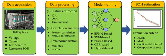
Figure 2.
Procedures for developing data-driven SOH estimation algorithms.
In summary, two key processes for building an accurate data-driven SOH estimation method are health feature extraction and ML algorithm implementation. How to extract high-related and easy-obtained features is the basis for developing a data-driven SOH estimation method and has become a current research hotspot. The current selection of aging features can be divided into three categories:
- (1)
- Features extracted from voltage and temperature curves during the charging and discharging process, especially the constant–current constant–voltage (CCCV) charging and constant–current (CC) discharging processes. For example, Cui et al. [11] extracted eight HFs from the voltage and temperature curves during CC discharging process and built a SOH estimation method. Liu et al. [12] used the discharging voltage difference of equal time intervals as an HF. However, the CC discharging mode rarely occurs in practical applications, making these HFs unusable for EV operations. Cao et al. [13] first analyzed the CC charging and constant–voltage (CV) charging phases, respectively, and then extracted seventeen HFs. The results of Grey relational analysis concluded that the HFs extracted from the CV phase were less closely related to battery degradation. According to the geometrical analysis of the complete CCCV charging profile, Yang et al. [14] extracted four HFs, such as the time of CC mode, the time of CV mode, the slope of the curve at the end of CC charging mode, and the vertical slope at the corner of the CC charging curve. Undeniably, the HFs extracted from the complete CCCV charging profile can reflect the battery degradation, but for the actual charging condition of EVs, the initial charging SOC is not necessarily 0%, and the terminal charging SOC is not 100%.
- (2)
- Features extracted from constructed curves, such as incremental capacity (IC) curve [15], differential voltage (DV) curve [16], and differential temperature (DT) curve [17]. Take the IC curve as an example. Because the IC curve has prominent peaks, many studies have selected relevant features as the HFs to build data-driven SOH estimation methods. For example, Li et al. [18] extracted eleven HFs in the voltage range from 3.8 V to 4.1 V at the voltage interval of 30 mV. Zhao et al. [19] selected the peak and valley values as HFs to construct the SOH prediction method. Moreover, other geometrical characteristics, such as the width of the peak [20], the area under the peak [21], and the slope of the peak [22] are considered HFs. Although valuable features can be extracted from these constructed curves, these curves are easily disturbed by noise in actual operations. Additionally, an appropriate filtering algorithm is required to smooth the original curve, and then accurate HFs can be identified.
- (3)
- Features obtained from electrochemical impedance, or parameters of the ECM, such as polarization capacitance, polarization resistance, and ohmic resistance. For example, Lyu et al. [23] utilized the recursive least squares (RLS) method to identify the parameters of the Thevenin model. The identified ohmic and polarization resistance were used as HFs to train a linear regression model. Similarly, Yang et al. [24] chose ohmic resistance, polarization resistance, polarization capacitance, and state of charge (SOC) as the inputs of the particle swam optimization-least square support vector regression (PSO-LSSVR) method to estimate SOH. Generally, these features need to be identified using additional algorithms, which increases its difficulty in practical applications.
In addition, other HFs, such as sample entropy [25], and Kullback–Leibler distance [26], are employed to reflect the aging states of LiBs. Based on the above review, there are some principles to bear in mind when choosing HFs [27]: (1) suitability for practical working conditions; (2) easy access to acquire; (3) strong adaptability and robustness; (4) considering thermal factor; and (4) high relevant degree. Therefore, this paper employs a multi-feature extraction strategy to extract HFs from partial charging voltage, capacity, and temperature curves to match these principles.
After selecting HFs and constituting the training dataset, different data-driven methods are used to train the SOH estimation model. Widely used ML methods include:
- (1)
- Shallow neural networks (NNs), such as backpropagation neural network (BPNN) [28], extreme learning machine (ELM) [29], radial basis function neural network (RBFNN) [30], are employed owing to their simple implementation.
- (2)
- Deep learning (DL) methods, such as long-short term memory (LSTM) [31], gated recurrent unit (GRU) [32], and convolutional neural network (CNN) [33], are utilized owing to their superior accuracy, adaptation ability, and good generalization.
- (3)
- Probabilistic-based methods, such as Gaussian process regression (GPR) [34], and deep brief network (DBN) [13], are applied owing to their capability to provide the uncertainty of the estimated value.
- (4)
- Ensemble learning methods, such as random forest (RF) [17], AdaBoost [35], and gradient boosting decision tree (GBDT) [36], are used because they do not easily fall into over-fitting.
- (5)
- Support vector machine (SVM)-based methods [37,38] are utilized owing to their simple implementation and high accuracy.
Nonlinear autoregressive with exogenous input neural network (NARXNN) is a subclass of the recurrent neural network (RNN), which is suitable for predicting complex and nonlinear systems [39]. Compared to other RNNs, such as the LSTM and GRU, the NARXNN has a more straightforward structure, fewer parameters, and reasonable accuracy. Although many researchers employed the NARXNN for state of charge (SOC) estimation [40,41,42], only a few researchers applied it for SOH estimation. For example, Khaleghi et al. [43] utilized the open-mode NARXNN to capture the dependency between the HFs and battery SOH. In another work, Cui et al. [11] built the closed-mode NARXNN to estimate the battery SOH. Moreover, the existing methods have used a time-consuming trial-and-error approach for finding the appropriate hyperparameters, which is inefficient. Recently, an effective strategy for hyperparameter tuning has been to combine data-driven algorithms and heuristic optimization techniques. For example, Ren et al. [44] utilized the particle swarm optimization (PSO) algorithm to optimize the number of hidden neurons, the learning rate, and the maximum epochs of the LSTM. Zhang et al. [45] employed the PSO algorithm to optimize the kernel parameters (w and σ) of the RBFNN. Hossain et al. [46] used the gravitational search algorithm (GSA) to find the best number of hidden neurons of the ELM. Compared with other heuristic optimization techniques, the PSO algorithm has the advantages of easy implementation, strong robustness, and global exploration. Therefore, this paper attempts to use the PSO algorithm to find the best values of input delays, feedback delays, and the number of hidden neurons of the NARXNN. Then the NARXNN is employed to build a multi-feature-based SOH estimation model. In summary, the main contributions of this paper are as follows:
- To comprehensively describe the battery aging characteristics, a multi-feature extraction strategy is employed to extract HFs from partial voltage, capacity, and temperature curves. Qualitative and quantitative analysis is used to evaluate the selected HFs.
- The performance of the NARXNN is highly dependent on the number of input delays, feedback delays, and neurons in the hidden layer. Hence, the PSO algorithm is applied to improve the training efficiency of NARXNN by searching for the optimal values of input delays, feedback delays, and the number of hidden neurons.
- The SOH estimators based on a single feature and fusion feature are comprehensively compared to verify the validity of the muti-feature extraction strategy. Moreover, to verify the effectiveness of the proposed PSO-NARXNN, a simple three-layer BPNN and a conventional NARXNN are built for comparison.
2. Data Analysis and Feature Extraction
2.1. Oxford Battery Degradation Dataset
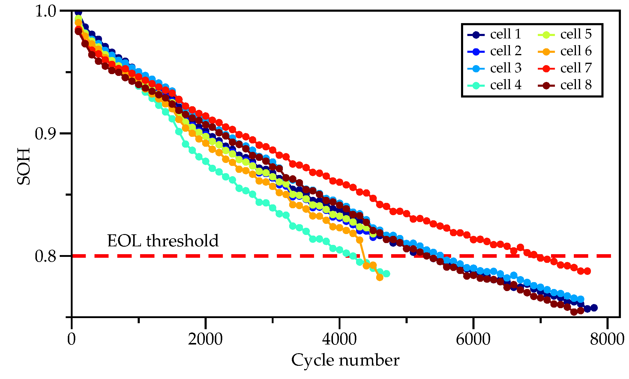
In this paper, a public dataset from the University of Oxford is utilized for LiBs aging analysis and SOH estimation algorithm development. As introduced in Ref. [47], the Oxford aging dataset contains measurements of battery aging data from eight Kokam pouch batteries with a nominal capacity of 740 mAh, noted as cell 1 to cell 8. The negative electrode material is graphite, and the positive electrode material is LiMO2 (where M means a combination of Ni, Co, and Mn, commercially known as NMC) [48]. The cells were all tested in a thermal chamber at 40 °C. The cells were exposed to a CCCV charging profile, followed by a drive cycle discharging profile obtained from the urban Artemis profile. Characterization measurements were taken every 100 cycles. The whole test procedure is summarized in Table 1. The voltage, current, and temperature data is recorded at a sampling interval of 1 s. More details can be found in Ref. [47]. The typical EOL threshold for LiBs is when the SOH decreases to 80%, and the LiBs are suggested to be retired. Hence, only the data with SOH higher than 80% are selected for LiBs aging analysis and SOH estimation algorithm development, as depicted in Figure 3. It is worth noting that even though these 8 LiBs with the same cathode material use the same aging experimental settings, the aging paths are significantly different. One possible reason for this phenomenon is internal variations in material properties from cell manufacturing. Another reason could be the effects of non-uniform environmental temperatures in the thermal chamber.

Table 1.
Test schedule of the Oxford dataset [49].

Figure 3.
SOH curves of cell 1 to cell 8.
2.2. Health Feature Extraction
The proposed multi-feature extraction strategy will be explained in detail in this section.
2.2.1. Voltage Feature Extraction
The terminal voltage and capacity curves of cell 1 under different aging states are shown in Figure 4. Note that only the CC charging phase is recorded in the Oxford dataset. Additionally, as concluded in Ref. [13], the HFs extracted from CC charging phase are more related to the battery SOH. Therefore, we only extract features from CC charging phase.

Figure 4.
(a) Terminal voltage curves of cell 1; (b) Charging capacity curves of cell 1.
As shown in Figure 4a, the time for LiBs to reach 4.2 V gradually decreases as the number of cycles increases, which directly reflects the reduction in usable capacity. This phenomenon can also be demonstrated in Figure 4b, where the charged capacity gradually decreases with the battery SOH decreases. Thus, the charged time and charged capacity of the CC phase can be selected as HFs. However, considering the practical operations of EVs, LiBs are rarely charged from 0% to 100% SOC but in a specific SOC range (e.g., 40% to 80%). Therefore, the charged time and charged capacity from partial CC curves of voltage varying from 3.8 V to 4.0 V (about 35% to 80% SOC) are selected as HFs to reflect the battery degradation, denoted as T1 and Q1, respectively.
2.2.2. Temperature Feature Extraction
As shown in Figure 5a, the raw temperature curves under different aging states are vulnerable to the impact of temperature sensor noise, resulting in difficulty in extracting temperature-related features. Therefore, a finite difference method is utilized in this paper to pre-process the raw temperature curves and then obtain the differential temperature (DT) curves [17]. The expression is as follows:
where is the pre-determined sample interval. Generally, when chooses a larger value, the DT curves cannot present subtle temperature changes. However, if takes a smaller value, the finite difference method cannot eliminate the influence of temperature sensor noise and produce errors. After parameter tuning, the interval sampling = 40 s is selected in this paper. In addition, a Gaussian filter is used to smooth the original DT curves to eliminate the impact of noise further.

Figure 5.
(a) Raw temperature curves of cell 1; (b) Smoothed DT curves of cell 1.
Figure 5b shows the DT curve of cell 1 under different aging states. Overall, the DT curve can be divided into three parts: (1) The DT curve first undergoes a period of rapid ascent, reaching its first peak value (denoted as F1); (2) After that, it undergoes a sharp decline and reaches its first valley value (denoted as F2); (3) Then, it experiences a rapid increase. Note that the DT curve represents the temperature change rate during the charging process. Thus, the entire DT curve shows a particular trend with the SOH decreases. Specifically, the first peak value, F1, gradually decreases, and the voltage corresponding to F1 (denoted as V1) increases with the SOH decreases. Moreover, the voltage corresponding to the valley value F2 (denoted as V2) gradually declines with the SOH decreases, but the valley value F2 does not show a clear upward or downward trend. In addition, the voltage difference between F1 and F2 (denoted as ΔV) shows a decreasing trend. As for the third part, although the DT curve shows an overall increasing trend and then declines, health features are not noticeable. Overall, the first and second parts of the DT curve present an obvious change with the SOH decreases. Therefore, the peak value F1, the voltage corresponding to F1, the voltage corresponding to F2, and the voltage difference ΔV between them, are chosen as HFs to describe the battery degradation.
2.2.3. IC Feature Extraction
The ICA is a widely used method to analyze the aging mechanism of LiBs from the electrochemical level. The IC curve is an effective tool for analyzing capacity loss and extracting HFs. The most important function of ICA is translating the flat capacity curve into the IC curve with clearly identifiable peaks, which can reflect the phase change characteristics of LiBs during active material insertion and delamination. Usually, the IC curve is obtained from the charging process under the CC charging phase by using a differential equation:
where Q represents the capacity, V denotes the voltage, and t is the sampling time.
As shown in Figure 6b, there are two peaks in the IC curve’s middle range (e.g., 3.4–4.0 V), and each peak can reflect the phase change inside the LiBs during the charging process with a 1-C charging rate. It can be found that the area under the peaks decreases with the cycle increases, indicating LAM and LLI [21]. In addition, the peak values decrease with a clear trend. Note that compared with the first peak (between 3.5 V and 3.7 V), the second peak (between 3.7 V and 4.0 V) shows a more noticeable trend during the aging process. Therefore, the value of the second peak (denoted as P1) and the area under the second peak between 3.7 V and 4.0 V (denoted as A1) are chosen as HFs to describe the degradation of battery capacity.

Figure 6.
(a) Charged capacity curves of cell 1; (b) Smoothed IC curves of cell 1.
2.2.4. Correlation Analysis
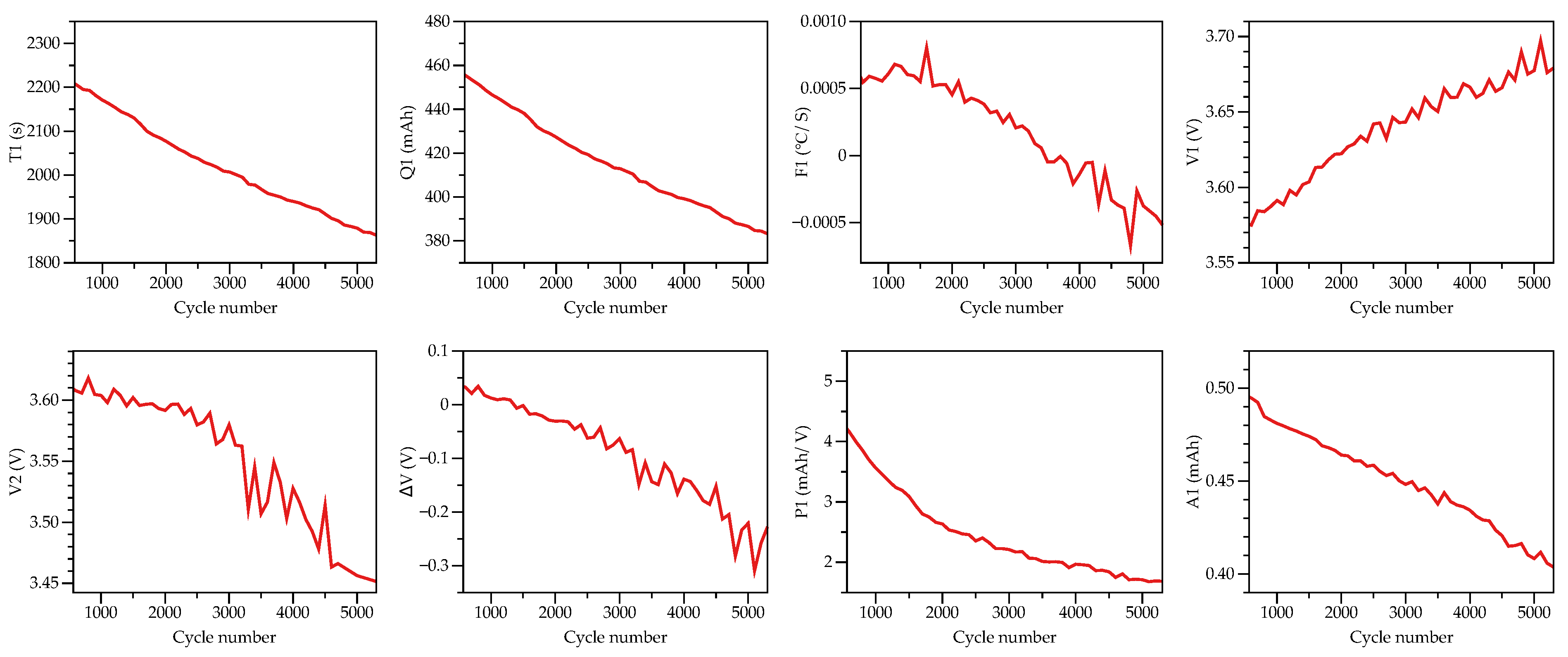
In summary, eight HFs are extracted from partial voltage, capacity, DT, and IC curves, respectively, which can match the feature-selecting principles mentioned in the Introduction. First, the voltage-related features are extracted from partial charging curves, which are suitable for practical conditions and easy to obtain. Second, the temperature-related features consider the thermodynamic factor. Third, the multi-feature extraction strategy can improve adaptability and robustness. Figure 7 shows the tendencies of the eight HFs of cell 1 with the increase of cycle numbers, which can reflect the qualitative relationship between HFs and battery SOH. It can be seen that only the V1 shows an upward trend, while other HFs all show a downward trend with the SOH decreases. In addition, HFs of other cells show a similar change trend as in Figure 7.
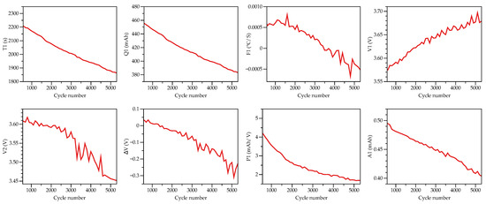
Figure 7.
Relationship between HFs and battery degradation.
To further evaluate the correlation of the selected HFs quantitatively, the Pearson correlation analysis is employed to calculate the correlation coefficient between the HFs and battery SOH. The equation is as follows:
where is the sequence of HF, is the sequence of battery SOH, and are their average values.
Table 2 summarizes the Pearson correlation coefficients between the HFs and battery SOH of eight cells. Generally, the absolute value of the correlation coefficient is closer to 1, indicating that the relational degree is greater. According to the correlation analysis results in Table 2, the absolute Pearson correlation coefficients of the HFs of eight cells are all greater than 0.9, indicating a high relational grade with the battery SOH. Therefore, using these HFs to build a data-driven method for SOH estimation is reasonable.

Table 2.
Correlation analysis results.
3. Related Algorithms
3.1. Nonlinear Autoregressive with Exogenous Input Neural Network
NARXNN is a sort of RNN that can learn to predict one time series by means of giving past values of the same time series and another time series called the external or exogenous time series. The structure of NARXNN is depicted in Figure 8, where TDL represents the time–delay line. According to the feedback mechanism of NARXNN, it can be regarded as a variant of the Jordan NN [50]. The expression of NARXNN is as follows:
where and are activation functions of the output layer and hidden layer respectively, and are weights and biases between the corresponding layers, and represent the input and feedback delays, respectively, and l is the number of hidden neurons.
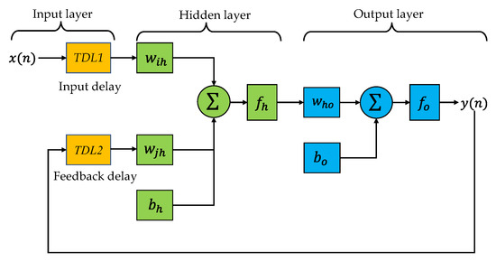
Figure 8.
Structure of NARXNN [43].
The most important hyperparameters of NARXNN are the input delays, feedback delays, number of hidden neurons, feedback mode, and training methods. In this paper, the input delays, feedback delays, and the number of hidden neurons are optimized using the PSO algorithm (introduced in the next section). Regarding the training methods, Levenberg–Marquardt (LM) and Bayesian regularization (BR) methods are the most convenient and common functions. Referring to [11], BR is chosen as the training function in this study. Regarding the feedback mode, there are two types: close and open. The former feeds back the predicted output to the input, while the latter feeds back the target output to the input. Although the open-mode NARXNN has a higher estimation theoretically, the close-mode NARXNN is adopted in this work because of the unavailability of the actual target in practical operations. In addition, the sigmoid transfer function and a linear transfer function are used at the hidden layer and output layer, respectively [51].
3.2. Particle Swarm Optimization
PSO was first proposed by Kennedy and Eberhart in 1995 [52]. Owing to its advantages of easy implementation and strong robustness, PSO has been employed in numerous applications. The basic idea of PSO is to search for the best results of particles with optimal values through an iterative process. Two locations are used for searching for the best solutions in PSO. The first is obtained through the current iteration, denoted as local best, pbest. The second is achieved in earlier iterations, denoted as global best, gbest. By calculating the objective function of each particle, the best pbest can be found in every iteration. Moreover, the best gbest can be found through a continuous update of particles. The position and velocity of every particle are updated as follows:
where and represent the velocity and position of ith particle at kth iteration, respectively, is the optimal solution of ith particle at kth iteration, is the global optimal solution of all particles until kth iteration, w represents weigh factor, and are random numbers between 0 and 1, and and are positive learning factor.
3.3. Flowchart of the PSO-NARXNN
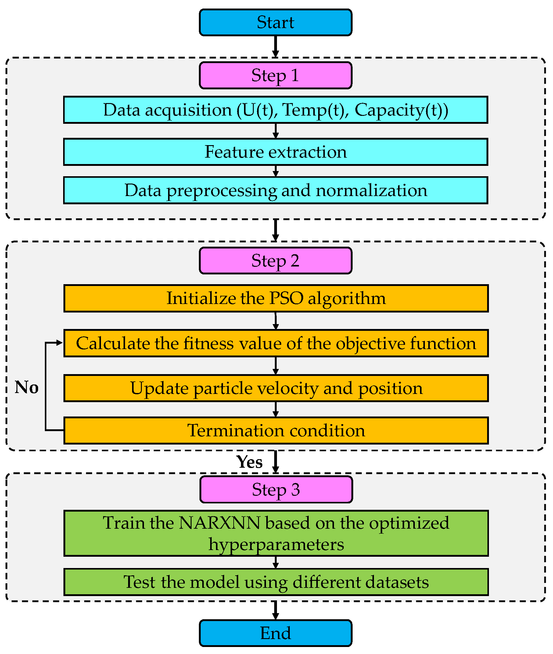
It is well-known that building a high-performance neural network requires appropriate hyperparameter settings. As for the NARXNN, input delays, feedback delays, and the number of hidden neurons are the three most essential hyperparameters determining its overall performance. Hence, in this paper, the PSO algorithm is applied to improve the performance of NARXNN by searching for the optimal value of input delays, feedback delays, and the number of hidden neurons. The flowchart of the PSO-NARXNN is depicted in Figure 9, and the specific steps are as follows:
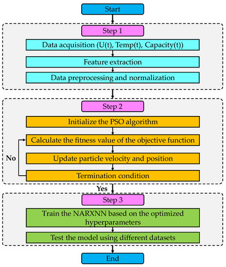
Figure 9.
Flowchart of the PSO-NARXNN.
Step 1: Data processing. Feature extraction and data normalization are the basis for model training. In this paper, the eight HFs mentioned in Section 2.2 are first extracted, then the Z-score normalization method is utilized to transform the original data to no-dimensional forms.
Step 2: PSO algorithm is used to optimize the hyperparameters of NARXNN.
- The main parameters of the PSO algorithm are assigned as follows: the particle dimension D is 3, population size N is 10, maximum iteration M is 100, the boundary limit of input and feedback delays is set between ‘1′ and ‘5′, and the boundary limit of hidden neurons is set between ‘1′ and ‘20′. Then, the initial position is generated randomly within the boundary.
- According to the initial position, which contains the values of input delays, feedback delays, and the number of hidden neurons, the NARXNN is trained based on BR algorithm. The mean square error (MSE) is taken as the objective function to calculate the fitness value, and the lowest value is considered ‘gbest’.
- The particle velocity and position are updated according to Equations (6) and (7), and then the fitness value is calculated to update the ‘pbest’ and ‘gbest’. In addition, the position of particles is verified by whether they are situated in the boundary.
- If the termination conditions are met, the algorithm ends and outputs the optimization results; otherwise, return to 3 in Step 2.
Step 3: The optimized hyperparameters are used to train the NARXNN. Then, the trained NARXNN is tested based on the testing datasets. Moreover, several statistical metrics are used to evaluate the model error. The experimental results will be discussed in the next section.
Note that MATLAB version 2022b (MathWorks, Natick, MA, USA) is used to develop all related algorithms proposed in this paper.
4. Results and Discussion
This section discusses the experimental results of the proposed muti-feature extraction strategy and PSO-NARXNN for SOH estimation. It should be noted that the reference SOH is calculated based on the CC charging characteristic test, as summarized in Table 1. Several statistical metrics, such as the mean absolute error (MAE), the root mean square error (RMSE), and the maximum error (MaxE), are employed to evaluate the estimation results quantitatively. The MAE can measure the average error size, while the RMSE describes the dispersion and convergence performance. The expressions are as follows:
where represents the predicted value, represents the reference value, and N is the number of samples.
To fully use the Oxford aging dataset and verify the generalization of the proposed SOH estimation method, the aging datasets of eight cells are constructed into eight groups for experiments. For example, experimental group 1 represents that the aging dataset of cell 1 is used as a training dataset for model training. Then, the aging datasets of the other seven cells are used as testing datasets. In this way, the feasibility of the selected HFs and the generalization of the proposed SOH method can be evaluated comprehensively.Section 4.1.1, Section 4.1.2 and Section 4.1.3 explain the results of group 1, and Section 4.1.4 gives the results of the other seven experimental groups.
4.1. Results
4.1.1. Optimal Parameters
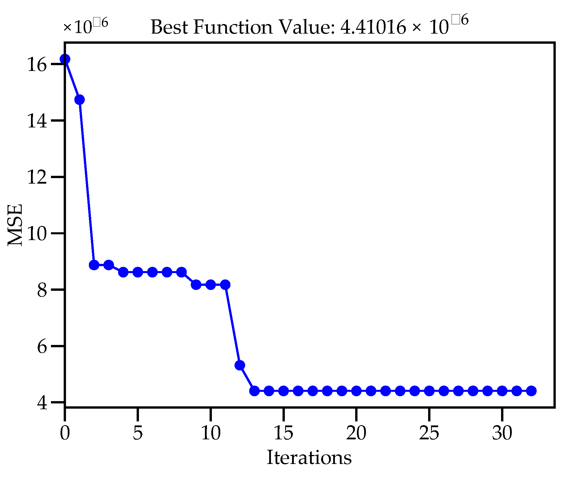
Firstly, the optimal values of input delays, output delays, and the number of hidden neurons are optimized by the PSO algorithm. The convergence curve is shown in Figure 10. It can be seen that the minimum value of the objective function is achieved after 32 iterations when the relative change in the objective function value over the last iteration is less than the tolerance. Moreover, the optimal values of input delays, output delays, and the number of hidden neurons are attained as 1, 2, and 15, respectively. Then, the NARXNN is trained using the optimal values and compared with other algorithms in the following sections.
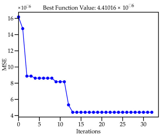
Figure 10.
Convergence curve of PSO algorithm.
4.1.2. Comparison with Different Feature Extraction Strategies
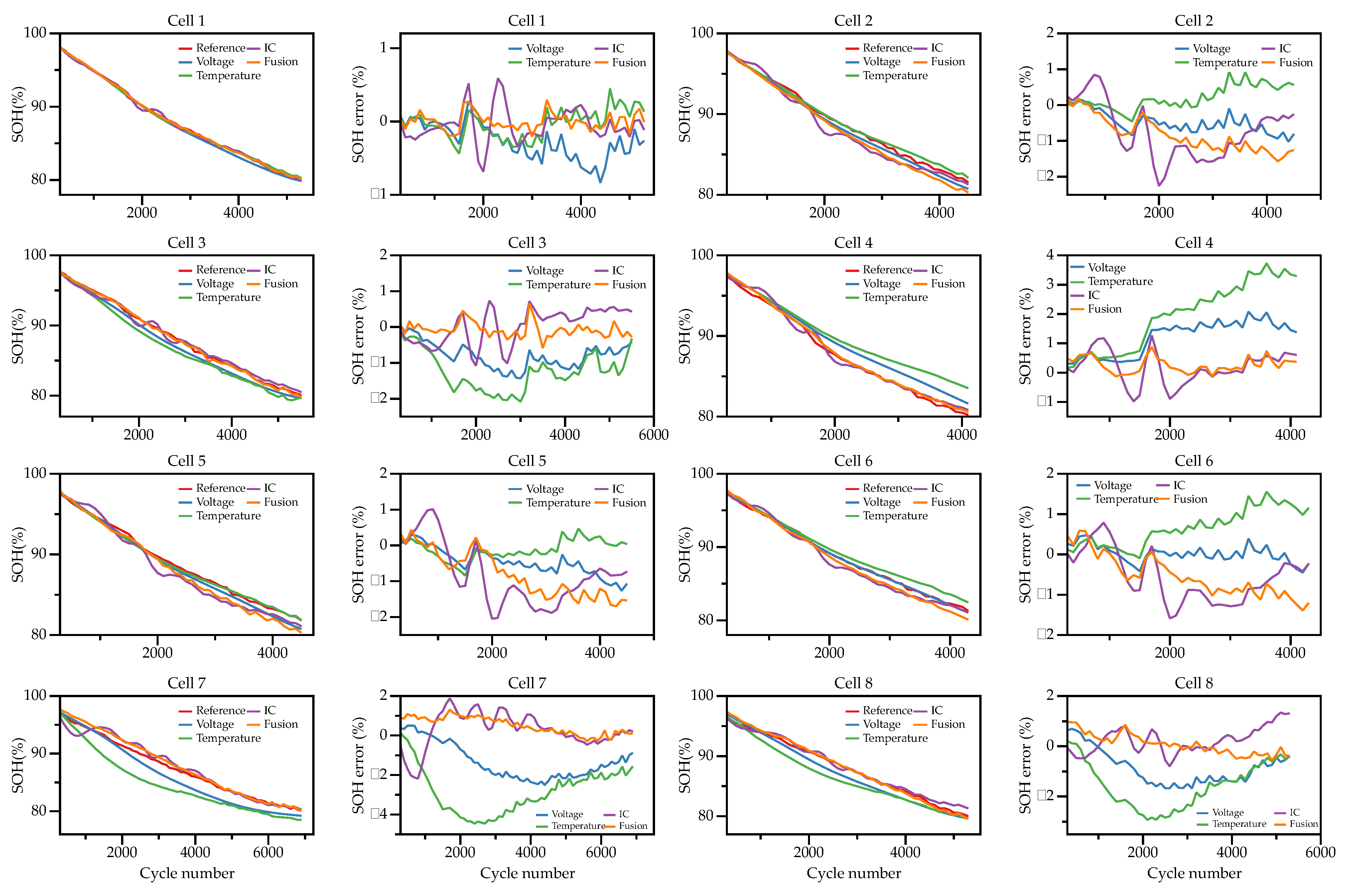
As mentioned in the Introduction, health feature extraction is essential for building a high-performance SOH estimation model. To verify the effectiveness of the proposed multi-feature extraction strategy, the voltage, temperature, IC, and fusion features are separately used to train the PSO-NARXNN and compared in this section. The SOH estimation results based on different feature extraction strategies are shown in Figure 11, and the statistical metrics are given in Table 3.
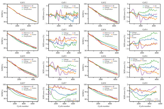
Figure 11.
SOH estimation results of different feature extraction strategies.

Table 3.
Summary of MAE and RMSE of different feature extraction strategies.
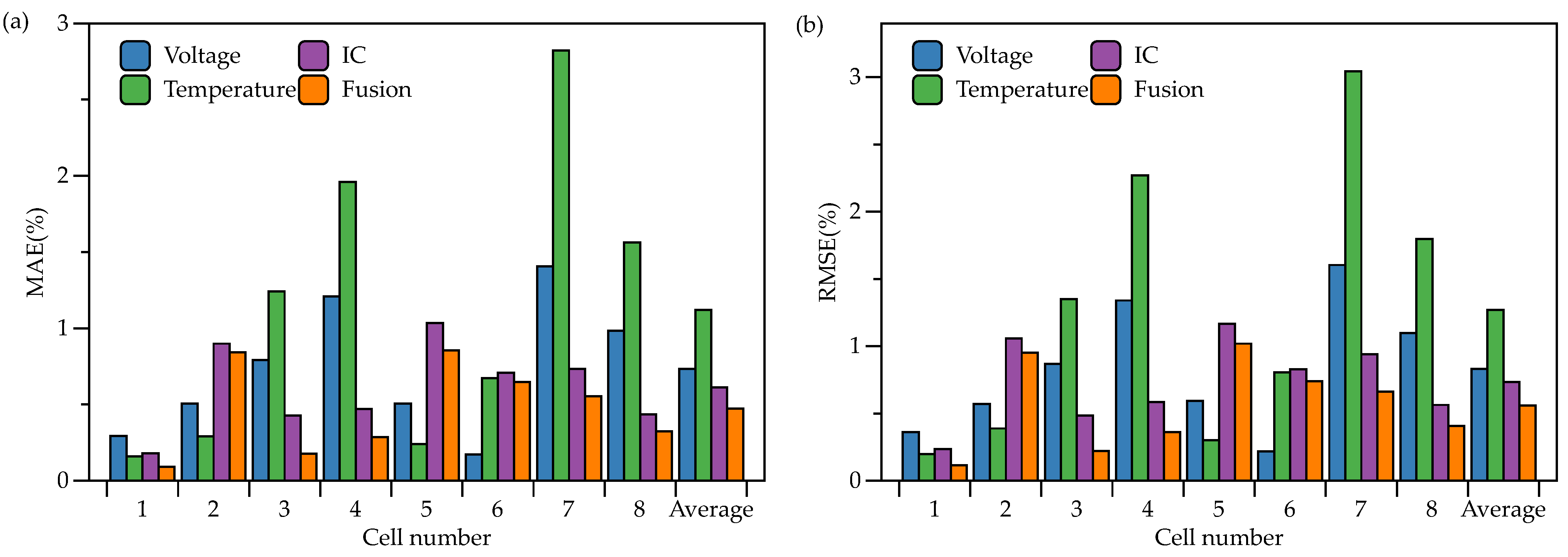
Overall, the fusion feature-based method can obtain accurate and robust estimation results under all testing datasets. In contrast, single feature-based methods can only achieve acceptable estimation results on specific testing datasets. For example, the temperature feature-based method can obtain great estimation accuracy for cell 2 and cell 5 with the MAEs less than 0.3% and RMSEs less than 0.4%. However, the estimation results of other cells are the worst, where the MAEs of cell 3, cell 4, cell 7, and cell 8 are 1.24%, 1.96%, 2.82%, and 1.56%, respectively, while the RMSEs are 1.35%, 2.27%, 3.04%, and 1.80%, respectively. Moreover, the MaxE of cell 7 exceeds 4%, which is unacceptable. The DT curve can reflect the thermodynamic characteristics of LiBs during the degradation process. However, the differential operation may magnify the noise in measurement, and the filtering algorithm may influence the feature extraction process. Thus, only using the temperature feature cannot obtain accurate and robust estimation results for all testing datasets. Regarding the voltage feature, the overall estimation performance is better than the temperature feature, according to the error curves in Figure 11. However, only using the voltage feature cannot guarantee the estimation robustness under different testing datasets. It can be seen that the MAE of cell 6 achieves the lowest value, while the MAEs of cell 4 and cell 7 exceed 1%. The MaxEs of cell 4 and cell 7 exceed 2%. Regarding the IC feature, the IC curve can describe the electrochemical characteristics of LiBs during the aging process. It can be seen that the overall SOH estimation results based on the IC feature are better than the temperature and voltage features, especially for cell 3, cell 4, cell 7, and cell 8. However, compared with the fusion feature-based method, the error curves of the IC feature-based method show more fluctuations, resulting in larger RMSEs and MaxEs, where the MaxEs of cell 2, cell 5, and cell 7 exceed 2%. Finally, the multi-feature extraction strategy can fully use the advantages of different kinds of features and avoid their disadvantages, resulting in more accurate and robust estimation results. It can be seen from Figure 12 that although the MAEs of the fusion feature-based method for cell 2 and cell 5 are not the lowest, it remains within 1%. Moreover, the fusion feature-based method can obtain the best estimation performance for other cells. The average MAE of the fusion feature-based method is 0.47%, which is 57.79%, 35.63%, and 22.73% lower than the temperature, voltage, and IC feature-based methods, respectively. As such, the effectiveness of the proposed multi-feature extraction strategy is verified based on the above analysis.
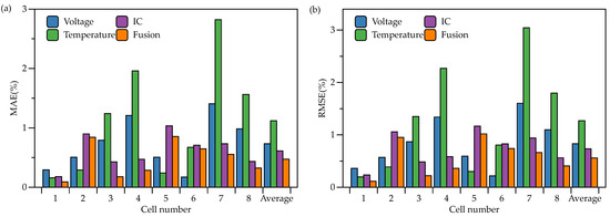
Figure 12.
(a) MAE of different feature extraction strategies; (b) RMSE of different feature extraction strategies.
4.1.3. Comparison with Different Algorithms
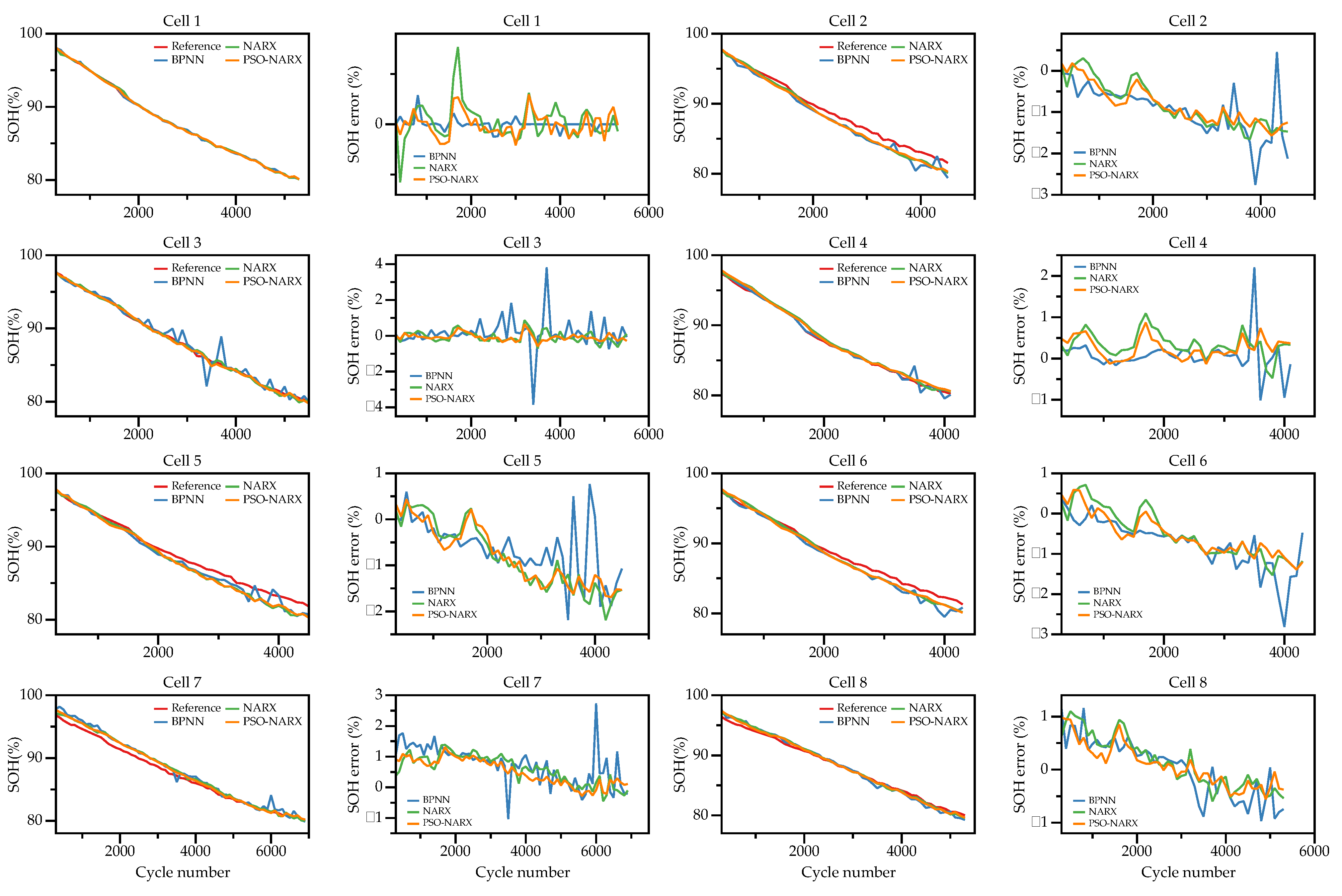
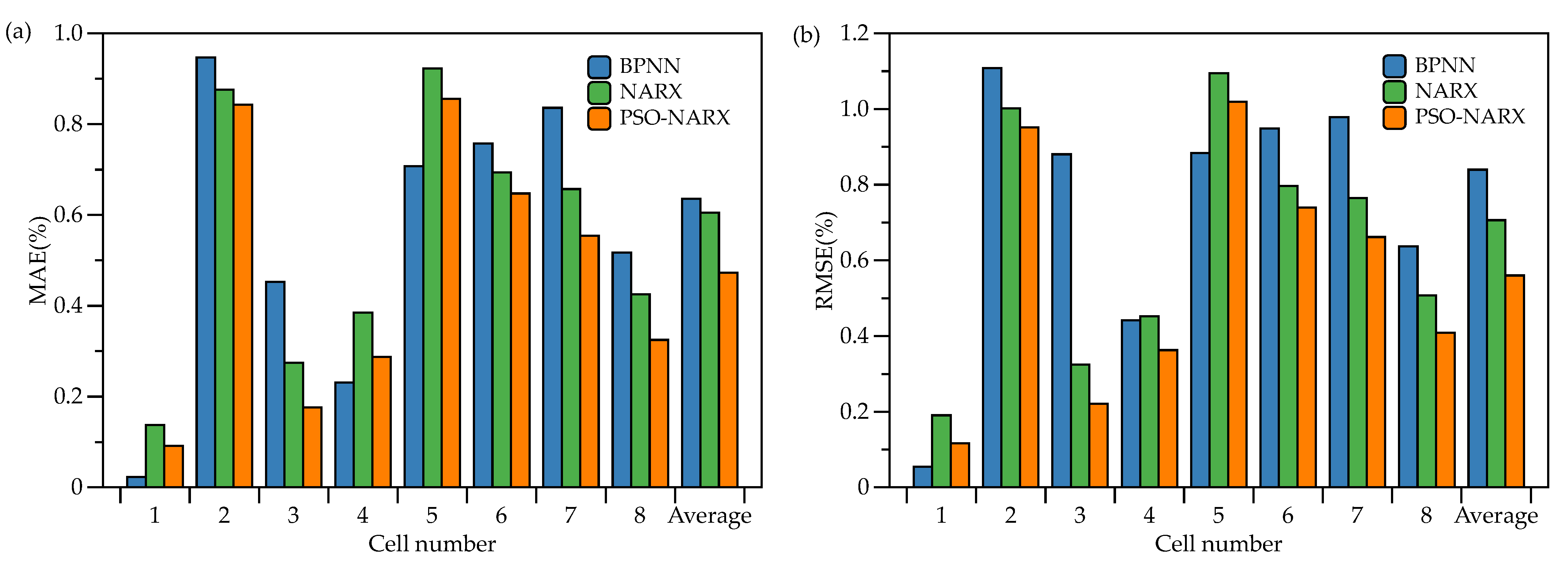
As concluded in Section 4.1.1, the optimal values of input delays, feedback delays, and the number of hidden neurons are optimized by the PSO algorithm. To verify the effectiveness of the optimal hyperparameters, a conventional NARXNN whose input delays, feedback delays, and the number of hidden neurons are randomly assigned is built for comparison. Additionally, to further verify the validity of the selected HFs, a simple three-layer BPNN is trained for comparison, too. For a fair comparison, the hyperparameters and training settings of the above two methods, including the number of hidden neurons, activation function, and training method, are entirely consistent with the PSO-NARXNN method. Figure 13 shows the SOH estimation results, and Figure 14 visually compares the MAE and RMSE of the above three methods. The statistical metrics are given in Table 4.
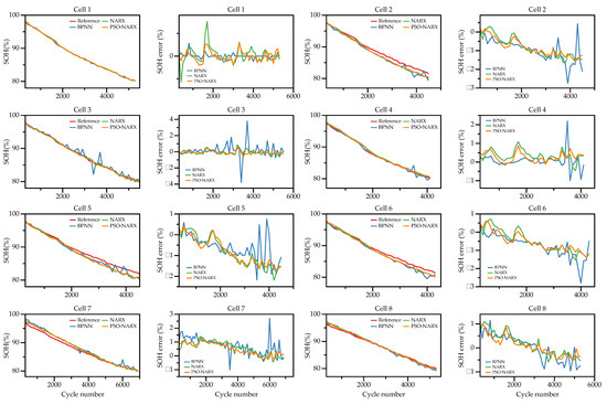
Figure 13.
SOH estimation results of different algorithms.
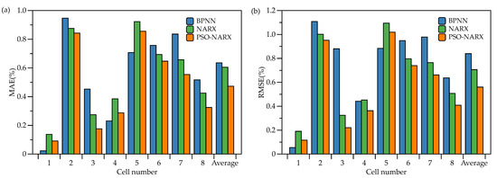
Figure 14.
(a) MAE of different algorithms; (b) RMSE of different algorithms.

Table 4.
Summary of MAE and RMSE of different algorithms.
According to the SOH estimation curves shown in Figure 13, the estimated SOH of the three methods can generally follow the aging path. However, the SOH curves estimated based on the PSO-NARXNN method have better consistency and smoothness with the real SOH trajectory. In contrast, the estimated curves based on the BPNN and conventional NARXNN methods show different degrees of fluctuations. Specifically, regarding the BPNN method, the MAEs of all cells are less than 1%, and only the RMSE of cell 2 exceeds 1%, indicating 1.10%. Moreover, the MAEs of cell 4 and cell 5 achieve the lowest values among the three methods. Therefore, the effectiveness of the proposed multi-feature extraction strategy is further verified because a simple BPNN can obtain a relatively satisfactory estimation performance. However, the MaxEs of the BPNN method are all larger than 2%, and the estimated SOH curves show significant fluctuations, especially during the EOL of LiBs, according to the error curves in Figure 13. As a result of the fluctuation, the BPNN method has an average MAE and RMSE of 0.64% and 0.84%, which are larger than the other two methods. Regarding the conventional NARXNN method, it can achieve an overall better performance in comparison to the BPNN method. Especially, the estimation errors of cell 3 and cell 7 are reduced to a larger extent. The average MAE is 0.60%, 6.7% lower than the BPNN method. Moreover, the average RMSE is 0.70%, which is 16.7% lower than the BPNN method. In addition, according to the error curves in Figure 13, the MaxEs of the conventional NARXNN method are all less than those of the BPNN method, showing a more robust estimation result. This is because the feedback mechanism of the NARXNN can learn information from the past values of output and previous values of exogenous input data. Regarding the PSO-NARXNN, it can be seen from Figure 14 that all MAEs and RMSEs are reduced in comparison to the conventional NARXNN. The error curves in Figure 13 also demonstrate that the PSO-NARXNN has an overall better estimation performance than the conventional NARXNN. The MAE of cell 3 reaches the lowest value, 0.17%. The average MAE and RMSE are 0.47% and 0.56%, which are 21.67% and 20% lower than the conventional NARXNN method and 26.56% and 33.33% lower than the BPNN method. Therefore, the effectiveness of the PSO algorithm is verified.
In summary, by comparing the BPNN and conventional NARXNN methods, the effectiveness of the multi-feature extraction strategy is further demonstrated. Moreover, by comparing the conventional NARXNN and PSO-NARXNN methods, the effectiveness of the optimal values by the PSO algorithm is verified.
4.1.4. Results of Other Experimental Groups
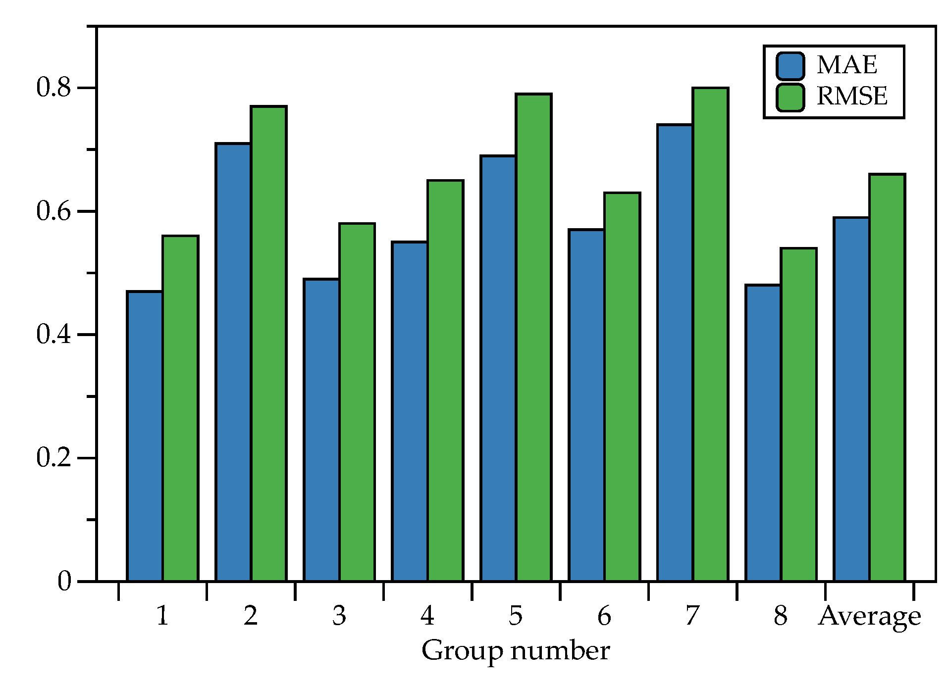
As explained at the beginning of Section 4, there are eight experimental groups to comprehensively evaluate the effectiveness of the proposed multi-feature extraction strategy and PSO-NARXNN model. Section 4.1.2 and 4.1.3 has discussed the experimental results of group 1, which uses the aging dataset of cell 1 to train the model, and then the aging datasets of the other seven cells to test it. In this section, the results of other experimental groups are explained. Owing to space limitation, the average MAE and RMSE of 7 experimental groups are given in Table 5, and Figure 15 intuitively compares them.

Table 5.
Summary of MAE and RMSE of other experimental groups.
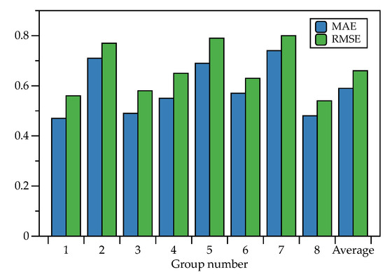
Figure 15.
Comparison of MAE and RMSE of other experimental groups.
As shown in Figure 15, it can be seen that average MAE and RMSE are all less than 1%, which means that no matter which cell aging dataset is used to train the PSO-NARXNN SOH estimation model, it can achieve excellent estimation accuracy for other aging datasets. This result demonstrates the generalization of the proposed PSO-NARXNN SOH estimation method and proves that the multi-feature extraction strategy is valid for different cells. This conclusion also coincides with the observation in the above two sections. To further validate the superior performance of the proposed PSO-NARXNN method, similar methods, especially those with SOH estimation works based on the Oxford dataset, are compared in Table 6. It is evident from Table 6 that the proposed method has higher or at least comparable accuracy than those of other existing approaches. In addition, as explained in the Introduction, the NARXNN has a more straightforward structure and fewer parameters than the GRU, CNN, and RF regressor.

Table 6.
Comparison with other similar works.
Overall, the analysis above comprehensively verifies the effectiveness of the multi-feature extraction strategy and the proposed PSO-NARXNN SOH estimation method on the Oxford aging dataset.
4.2. Discussion
The above results demonstrate the validity of the multi-feature extraction strategy and the performance of the PSO-NARXNN for SOH estimation, but there are still some limitations and shortcomings. First, the selected HFs and the proposed method are verified on one type of LiB. The feasibility on other types of LiBs needs to be further validated. Second, it can be concluded from Section 4.1.3 that a simple three-layer BPNN can obtain a relatively satisfactory estimation accuracy when the HFs are reasonable. Therefore, how to further optimize the HFs and then achieve high-precision estimation using only a simple algorithm deserves further investigation. Third, this research only focuses on SOH estimation methods for cell, while SOH estimation methods for the battery pack are not covered. More studies need to determine whether the selected HFs are suitable for battery pack SOH estimation. Additionally, the computation requirements would become larger when applying the cell estimation method to pack estimation. How to maintain a trade-off between model accuracy and complexity deserves further investigation. Therefore, our future work will employ other aging datasets, such as the NASA dataset [56] and CALCE (Center Advanced Life Cycle Engineering) dataset [57], to validate the feasibility of the proposed multi-feature extraction strategy as well as the PSO-NARXNN. In addition, SOH estimation methods for the battery pack will be investigated based on the research in this paper.
5. Conclusions
To improve the SOH estimation performance, this paper proposes a multi-feature extraction strategy and PSO-NARXNN for accurate SOH estimation of LiBs. Firstly, eight HFs are extracted from partial voltage, capacity, DT, and IC curves to reflect the battery aging process comprehensively. Then, qualitative and quantitative analyses are used to evaluate the effectiveness of the selected HFs. Second, owing to the advantages of simple structure, easy implementation, and high estimation accuracy, the NARXNN is adopted to build an accurate SOH estimation model. To improve the training efficiency, the PSO algorithm is applied to optimize the hyperparameters of NARXNN, including input delays, feedback delays, and the number of hidden neurons. Finally, the proposed multi-feature extraction strategy and PSO-NARXNN are systematically validated using the Oxford aging dataset. The results show that in comparison to a simple three-layer BPNN and a conventional NARXNN, the proposed PSO-NARXNN can achieve higher accuracy and stronger robustness, where the average MAE and RMSE of eight experimental groups are 0.59% and 0.66%, respectively.
Our future work will use other types of LiBs to validate the proposed multi-feature extraction strategy and PSO-NARXNN method. Moreover, the multi-feature extraction strategy will be further optimized, and a simpler algorithm will be used for accurate SOH estimation. Then, the optimized algorithm will be used for battery pack SOH estimation.
Author Contributions
Conceptualization, Z.R. and C.D.; Funding acquisition, C.D. and W.R.; Methodology, Z.R.; Software, Z.R.; Supervision, C.D. and W.R.; Validation, Z.R.; Visualization, Z.R.; Writing—original draft, Z.R.; Writing—review and editing, Z.R., C.D. and W.R. All authors have read and agreed to the published version of the manuscript.
Funding
This research was funded by the Key R&D project of Hubei Province China, grant number 2021AAA006; Foshan Xianhu Laboratory of the Advanced Energy Science and Technology Guangdong Laboratory, grant number XHD2020-003.
Data Availability Statement
The data of this paper are available on the following website: https://ora.ox.ac.uk/objects/uuid:03ba4b01-cfed-46d3-9b1a-7d4a7bdf6fac (accessed on 2 November 2022).
Conflicts of Interest
The authors declare no conflict of interest.
References
- Balasingam, B.; Ahmed, M.; Pattipati, K. Battery Management Systems-Challenges and Some Solutions. Energies 2020, 13, 2825. [Google Scholar] [CrossRef]
- Pastor-Fernández, C.; Yu, T.F.; Widanage, W.D.; Marco, J. Critical Review of Non-Invasive Diagnosis Techniques for Quantification of Degradation Modes in Lithium-Ion Batteries. Renew. Sustain. Energy Rev. 2019, 109, 138–159. [Google Scholar] [CrossRef]
- Waldmann, T.; Iturrondobeitia, A.; Kasper, M.; Ghanbari, N.; Aguesse, F.; Bekaert, E.; Daniel, L.; Genies, S.; Gordon, I.J.; Löble, M.W.; et al. Review—Post-Mortem Analysis of Aged Lithium-Ion Batteries: Disassembly Methodology and Physico-Chemical Analysis Techniques. J. Electrochem. Soc. 2016, 163, A2149–A2164. [Google Scholar] [CrossRef]
- Han, X.; Lu, L.; Zheng, Y.; Feng, X.; Li, Z.; Li, J.; Ouyang, M. A Review on the Key Issues of the Lithium Ion Battery Degradation among the Whole Life Cycle. eTransportation 2019, 1, 100005. [Google Scholar] [CrossRef]
- Che, Y.; Deng, Z.; Li, P.; Tang, X.; Khosravinia, K.; Lin, X.; Hu, X. State of Health Prognostics for Series Battery Packs: A Universal Deep Learning Method. Energy 2022, 238, 121857. [Google Scholar] [CrossRef]
- Xiong, R.; Li, L.; Tian, J. Towards a Smarter Battery Management System: A Critical Review on Battery State of Health Monitoring Methods. J. Power Sources 2018, 405, 18–29. [Google Scholar] [CrossRef]
- Ren, Z.; Du, C.; Wu, Z.; Shao, J.; Deng, W. A Comparative Study of the Influence of Different Open Circuit Voltage Tests on Model-Based State of Charge Estimation for Lithium-Ion Batteries. Int. J. Energy Res. 2021, 45, 13692–13711. [Google Scholar] [CrossRef]
- Vennam, G.; Sahoo, A.; Ahmed, S. A Novel Coupled Electro-Thermal-Aging Model for Simultaneous SOC, SOH, and Parameter Estimation of Lithium-Ion Batteries. In Proceedings of the 2022 American Control Conference (ACC), Atlanta, GA, USA, 8–10 June 2022; pp. 5259–5264. [Google Scholar]
- Zeng, M.; Zhang, P.; Yang, Y.; Xie, C.; Shi, Y. SOC and SOH Joint Estimation of the Power Batteries Based on Fuzzy Unscented Kalman Filtering Algorithm. Energies 2019, 12, 3122. [Google Scholar] [CrossRef]
- Sui, X.; He, S.; Vilsen, S.B.; Meng, J.; Teodorescu, R.; Stroe, D.I. A Review of Non-Probabilistic Machine Learning-Based State of Health Estimation Techniques for Lithium-Ion Battery. Appl. Energy 2021, 300, 117346. [Google Scholar] [CrossRef]
- Cui, Z.; Wang, C.; Gao, X.; Tian, S. State of Health Estimation for Lithium-Ion Battery Based on the Coupling-Loop Nonlinear Autoregressive with Exogenous Inputs Neural Network. Electrochim. Acta 2021, 393, 139047. [Google Scholar] [CrossRef]
- Liu, D.; Zhou, J.; Liao, H.; Peng, Y.; Peng, X. A Health Indicator Extraction and Optimization Framework for Lithium-Ion Battery Degradation Modeling and Prognostics. IEEE Trans. Syst. Man, Cybern. Syst. 2015, 45, 915–928. [Google Scholar] [CrossRef]
- Cao, M.; Zhang, T.; Wang, J.; Liu, Y. A Deep Belief Network Approach to Remaining Capacity Estimation for Lithium-Ion Batteries Based on Charging Process Features. J. Energy Storage 2022, 48, 103825. [Google Scholar] [CrossRef]
- Yang, D.; Zhang, X.; Pan, R.; Wang, Y.; Chen, Z. A Novel Gaussian Process Regression Model for State-of-Health Estimation of Lithium-Ion Battery Using Charging Curve. J. Power Sources 2018, 384, 387–395. [Google Scholar] [CrossRef]
- Li, X.; Wang, Z.; Yan, J. Prognostic Health Condition for Lithium Battery Using the Partial Incremental Capacity and Gaussian Process Regression. J. Power Sources 2019, 421, 56–67. [Google Scholar] [CrossRef]
- Wang, Z.; Yuan, C.; Li, X. Lithium Battery State-of-Health Estimation via Differential Thermal Voltammetry with Gaussian Process Regression. IEEE Trans. Transp. Electrif. 2021, 7, 16–25. [Google Scholar] [CrossRef]
- Lin, M.; Wu, D.; Meng, J.; Wu, J.; Wu, H. A Multi-Feature-Based Multi-Model Fusion Method for State of Health Estimation of Lithium-Ion Batteries. J. Power Sources 2022, 518, 230774. [Google Scholar] [CrossRef]
- Li, X.; Yuan, C.; Li, X.; Wang, Z. State of Health Estimation for Li-Ion Battery Using Incremental Capacity Analysis and Gaussian Process Regression. Energy 2020, 190, 116467. [Google Scholar] [CrossRef]
- Zhao, Q.; Jiang, H.; Chen, B.; Wang, C.; Chang, L. Research on the SOH Prediction Based on the Feature Points of Incremental Capacity Curve. J. Electrochem. Soc. 2021, 168, 110554. [Google Scholar] [CrossRef]
- Yang, S.; Luo, B.; Wang, J.; Kang, J.; Zhu, G. State of Health Estimation for Lithium-Ion Batteries Based on Peak Region Feature Parameters of Incremental Capacity Curve. Diangong Jishu Xuebao/Transactions China Electrotech. Soc. 2021, 36, 2277–2287. [Google Scholar] [CrossRef]
- Zhou, R.; Zhu, R.; Huang, C.G.; Peng, W. State of Health Estimation for Fast-Charging Lithium-Ion Battery Based on Incremental Capacity Analysis. J. Energy Storage 2022, 51, 104560. [Google Scholar] [CrossRef]
- Zhang, S.; Zhai, B.; Guo, X.; Wang, K.; Peng, N.; Zhang, X. Synchronous Estimation of State of Health and Remaining Useful Lifetime for Lithium-Ion Battery Using the Incremental Capacity and Artificial Neural Networks. J. Energy Storage 2019, 26, 100951. [Google Scholar] [CrossRef]
- Lyu, Z.; Wang, G.; Tan, C. A Novel Bayesian Multivariate Linear Regression Model for Online State-of-Health Estimation of Lithium-Ion Battery Using Multiple Health Indicators. Microelectron. Reliab. 2022, 131, 114500. [Google Scholar] [CrossRef]
- Yang, D.; Wang, Y.; Pan, R.; Chen, R.; Chen, Z. State-of-Health Estimation for the Lithium-Ion Battery Based on Support Vector Regression. Appl. Energy 2018, 227, 273–283. [Google Scholar] [CrossRef]
- Cao, M.; Zhang, T.; Yu, B.; Liu, Y. A Method for Interval Prediction of Satellite Battery State of Health Based on Sample Entropy. IEEE Access 2019, 7, 141549–141561. [Google Scholar] [CrossRef]
- Lin, M.; Zeng, X.; Wu, J. State of Health Estimation of Lithium-Ion Battery Based on an Adaptive Tunable Hybrid Radial Basis Function Network. J. Power Sources 2021, 504, 230063. [Google Scholar] [CrossRef]
- Fan, L.; Wang, P.; Cheng, Z. A Remaining Capacity Estimation Approach of Lithium-Ion Batteries Based on Partial Charging Curve and Health Feature Fusion. J. Energy Storage 2021, 43, 103115. [Google Scholar] [CrossRef]
- Kashkooli, A.G.; Fathiannasab, H.; Mao, Z.; Chen, Z. Application of Artificial Intelligence to State-of-Charge and State-of-Health Estimation of Calendar-Aged Lithium-Ion Pouch Cells. J. Electrochem. Soc. 2019, 166, A605–A615. [Google Scholar] [CrossRef]
- Ren, Z.; Du, C. State of Charge Estimation for Lithium-Ion Batteries Using Extreme Learning Machine and Extended Kalman Filter. IFAC Pap. 2022, 55, 197–202. [Google Scholar] [CrossRef]
- Mao, L.; Hu, H.; Chen, J.; Zhao, J.; Qu, K.; Jiang, L. Online State of Health Estimation Method for Lithium-Ion Battery Based on CEEMDAN for Feature Analysis and RBF Neural Network. IEEE J. Emerg. Sel. Top. Power Electron. 2021, 6777. [Google Scholar] [CrossRef]
- Kim, S.; Choi, Y.Y.; Kim, K.J.; Choi, J. Il Forecasting State-of-Health of Lithium-Ion Batteries Using Variational Long Short-Term Memory with Transfer Learning. J. Energy Storage 2021, 41, 102893. [Google Scholar] [CrossRef]
- Rouhi Ardeshiri, R.; Ma, C. Multivariate Gated Recurrent Unit for Battery Remaining Useful Life Prediction: A Deep Learning Approach. Int. J. Energy Res. 2021, 45, 16633–16648. [Google Scholar] [CrossRef]
- Yang, Y. A Machine-Learning Prediction Method of Lithium-Ion Battery Life Based on Charge Process for Different Applications. Appl. Energy 2021, 292, 116897. [Google Scholar] [CrossRef]
- Liu, K.; Li, Y.; Hu, X.; Lucu, M.; Widanage, W.D. Gaussian Process Regression with Automatic Relevance Determination Kernel for Calendar Aging Prediction of Lithium-Ion Batteries. IEEE Trans. Ind. Inform. 2020, 16, 3767–3777. [Google Scholar] [CrossRef]
- Li, R.; Li, W.; Zhang, H. State of Health and Charge Estimation Based on Adaptive Boosting Integrated with Particle Swarm Optimization/Support Vector Machine (AdaBoost-PSO-SVM) Model for Lithium-Ion Batteries. Int. J. Electrochem. Sci. 2022, 17, 1–17. [Google Scholar] [CrossRef]
- Qin, P.; Zhao, L.; Liu, Z. State of Health Prediction for Lithium-Ion Battery Using a Gradient Boosting-Based Data-Driven Method. J. Energy Storage 2022, 47, 103644. [Google Scholar] [CrossRef]
- Li, X.; Yuan, C.; Wang, Z. State of Health Estimation for Li-Ion Battery via Partial Incremental Capacity Analysis Based on Support Vector Regression. Energy 2020, 203, 117852. [Google Scholar] [CrossRef]
- Guo, Y.F.; Huang, K.; Hu, X.Y. A State-of-Health Estimation Method of Lithium-Ion Batteries Based on Multi-Feature Extracted from Constant Current Charging Curve. J. Energy Storage 2021, 36, 102372. [Google Scholar] [CrossRef]
- Sun, W.; Qiu, Y.; Sun, L.; Hua, Q. Neural Network-Based Learning and Estimation of Battery State-of-Charge: A Comparison Study between Direct and Indirect Methodology. Int. J. Energy Res. 2020, 44, 10307–10319. [Google Scholar] [CrossRef]
- Hannan, M.A.; Lipu, M.S.H.; Hussain, A.; Ker, P.J.; Mahlia, T.M.I.; Mansor, M.; Ayob, A.; Saad, M.H.; Dong, Z.Y. Toward Enhanced State of Charge Estimation of Lithium-Ion Batteries Using Optimized Machine Learning Techniques. Sci. Rep. 2020, 10, 4687. [Google Scholar] [CrossRef]
- Hossain Lipu, M.S.; Hussain, A.; Saad, M.H.M.; Ayob, A.; Hannan, M.A. Improved Recurrent NARX Neural Network Model for State of Charge Estimation of Lithium-Ion Battery Using Pso Algorithm. In Proceedings of the 2018 IEEE Symposium on Computer Applications & Industrial Electronics (ISCAIE), Penang, Malaysia, 28–29 April 2018; pp. 354–359. [Google Scholar] [CrossRef]
- Wang, Q.; Gu, H.; Ye, M.; Wei, M.; Xu, X. State of Charge Estimation for Lithium-Ion Battery Based on NARX Recurrent Neural Network and Moving Window Method. IEEE Access 2021, 9, 83364–83375. [Google Scholar] [CrossRef]
- Khaleghi, S.; Karimi, D.; Beheshti, S.H.; Hosen, M.S.; Behi, H.; Berecibar, M.; Van Mierlo, J. Online Health Diagnosis of Lithium-Ion Batteries Based on Nonlinear Autoregressive Neural Network. Appl. Energy 2021, 282, 116159. [Google Scholar] [CrossRef]
- Ren, X.; Liu, S.; Yu, X.; Dong, X. A Method for State-of-Charge Estimation of Lithium-Ion Batteries Based on PSO-LSTM. Energy 2021, 234, 121236. [Google Scholar] [CrossRef]
- Zhang, L.; Zheng, M.; Du, D.; Li, Y.; Fei, M.; Guo, Y.; Li, K. State-of-Charge Estimation of Lithium-Ion Battery Pack Based on Improved RBF Neural Networks. Complexity 2020, 2020, 8840240. [Google Scholar] [CrossRef]
- Hossain Lipu, M.S.; Hannan, M.A.; Hussain, A.; Saad, M.H.; Ayob, A.; Uddin, M.N. Extreme Learning Machine Model for State-of-Charge Estimation of Lithium-Ion Battery Using Gravitational Search Algorithm. IEEE Trans. Ind. Appl. 2019, 55, 4225–4234. [Google Scholar] [CrossRef]
- Christoph, R.B. Diagnosis and Prognosis of Degradation in Lithium-Ion Batteries. Ph.D. Thesis, Department of Engineering Science, University of Oxford, Oxford, UK, 2017. [Google Scholar]
- Birkl, C.R.; McTurk, E.; Roberts, M.R.; Bruce, P.G.; Howey, D.A. A Parametric Open Circuit Voltage Model for Lithium Ion Batteries. J. Electrochem. Soc. 2015, 162, A2271–A2280. [Google Scholar] [CrossRef]
- Chen, Z.; Zhao, H.; Zhang, Y.; Shen, S.; Shen, J.; Liu, Y. State of Health Estimation for Lithium-Ion Batteries Based on Temperature Prediction and Gated Recurrent Unit Neural Network. J. Power Sources 2022, 521, 230892. [Google Scholar] [CrossRef]
- Jordan, M.I. Serial Order: A Parallel Distributed Processing Approach; Ies Report 8604; Institute for Cognitive Science University of California: San Diego, CA, USA, 1986. [Google Scholar]
- Lipu, M.S.H.; Hannan, M.A.; Hussain, A.; Saad, M.H.M.; Ayob, A.; Blaabjerg, F. State of Charge Estimation for Lithium-Ion Battery Using Recurrent NARX Neural Network Model Based Lighting Search Algorithm. IEEE Access 2018, 6, 28150–28161. [Google Scholar] [CrossRef]
- Kennedy, J.; Eberhart, R. Particle Swarm Optimization. In Proceedings of the ICNN’95–International Conference on Neural Networks, Perth, WA, Australia, 27 November–01 December 1995; Volume 4, pp. 1942–1948. [Google Scholar]
- Fan, Y.; Xiao, F.; Li, C.; Yang, G.; Tang, X. A Novel Deep Learning Framework for State of Health Estimation of Lithium-Ion Battery. J. Energy Storage 2020, 32, 101741. [Google Scholar] [CrossRef]
- Goh, H.H.; Lan, Z.; Zhang, D.; Dai, W.; Kurniawan, T.A.; Goh, K.C. Estimation of the State of Health (SOH) of Batteries Using Discrete Curvature Feature Extraction. J. Energy Storage 2022, 50, 104646. [Google Scholar] [CrossRef]
- Gong, Q.; Wang, P.; Cheng, Z. An Encoder-Decoder Model Based on Deep Learning for State of Health Estimation of Lithium-Ion Battery. J. Energy Storage 2022, 46, 103804. [Google Scholar] [CrossRef]
- Saha, B.; Goebel, K. Battery Data Set; NASA Ames Prognostics Data Repository; NASA Ames: Moffett Field, CA, USA, 2007. Available online: http://ti.arc.nasa.gov/project/prognostic-data-repository (accessed on 5 November 2022).
- University of Maryland Battery Data|Center for Advanced Life Cycle Engineering (CALCE). Available online: https://calce.umd.edu/battery-data (accessed on 21 September 2021).
Disclaimer/Publisher’s Note: The statements, opinions and data contained in all publications are solely those of the individual author(s) and contributor(s) and not of MDPI and/or the editor(s). MDPI and/or the editor(s) disclaim responsibility for any injury to people or property resulting from any ideas, methods, instructions or products referred to in the content. |
© 2022 by the authors. Licensee MDPI, Basel, Switzerland. This article is an open access article distributed under the terms and conditions of the Creative Commons Attribution (CC BY) license (https://creativecommons.org/licenses/by/4.0/).

