Abstract
This paper presents battery aging models based on high-current incremental capacity features in the presence of battery cycling profiles characterized by fast charging conditions. In particular, the main peak area under the incremental capacity graph is proposed as a capacity indicator. A dataset from the Toyota Research Institute is analyzed. Batteries’ cycling data are characterized by various single- or double-step fast charges in constant current to reach 80% of the battery state of charge; the remaining charge process is performed by a 1C charge. Depending on the battery, a linear or logarithmic model was identified as the best suitable for representing the capacity–peak area relationship. The generalization capabilities of the proposed models are evaluated by performing an inference analysis of the fitting results over groups of batteries. Finally, we evaluated the prediction performance of the models by adopting a cross-validation approach.
1. Introduction
Multiple technical factors heavily limiting the widespread adoption of Electric Vehicles (EVs) are associated with the management and performance of batteries. Range anxiety, charge times and battery lifetime are very often identified as the three main factors that negatively impact the consumers’ perception of EVs. The reduction in flexibility and users’ comfort introduced by relatively long charge times, and the consequent reduction of willingness to use EVs, are part of the main arguments in favor of developing fast charging methods and infrastructures [1].
Fast charging requires high currents, which deeply increase battery degradation rates [2], due to the acceleration of processes such as lithium plating. The relationships between the fast charging protocol parameters and different battery aging mechanisms have been the topic of several research works [3,4,5]. In particular, multistep fast charging with a last step of 1C after reaching a given State of Charge (SoC) value has been shown to minimize the degradation rate induced by the use of high current rates during charging [4].
The increase in the charge current rates, and the associated rise on battery stress conditions, such as high temperatures, boosts the importance of proper battery monitoring and management, including the need for accurate and reliable battery capacity and State of Health (SoH) estimation. Recent literature classifies the methods usually employed for the estimation of battery capacity into three main groups: model-based, data-driven and experimental methods [6,7]. The usefulness of any of those approaches under a fast charge framework is defined by the inclusion of experiments or data with high current rates during the characterization or training stages.
Experimental battery capacity estimation methods typically require the characterization of the relationships between specific indicators and the battery capacity. Those relationships can be used later for estimating the capacity during normal usage of the battery. For a reliable estimation, the capacity indicator should be obtained regularly under similar operating conditions. In order to meet these requirements, usage scenarios that are repeated during typical operation need to be identified and characterized.
For example, the work in [8] proposes the times expended on fixed voltage ranges during a constant current (CC) charge as SoH indicators, using decision regression tree models for combining the results for multiple charge sections. The authors of [9] propose linear models linking the capacity with the variations of the battery surface temperature while charging. In the literature, multiple models for the estimation of the battery capacity, taking as input resistances computed during discharge current steps at fixed interval, have been proposed [10,11]. The features extracted from Incremental Capacity (IC) curves constitute a very popular family of capacity indicators in the recent literature [12,13]. Additionally, the parameters of models representing the voltage–IC relationship have been exploited as indicators for SoH estimation [14].
It is worth mentioning that such indicators have been identified for batteries aged without considering fast charging scenarios. Then, there is still a lack of models capable of relating the battery capacity and suitable indicators when considering degradation paths introduced by fast charging. In the case of batteries charged using multistep fast charging policies, such as the one studied in [4], the 1C CC final stage is an interesting candidate for capacity indicators analysis. In this stage, High-Current Incremental Capacity (HCIC) features can easily be computed [13]. Previously, for batteries aged without considering fast charging conditions, such features have been exploited for capacity estimation using relatively simple models, which is of interest for eventual on-board implementations.
Laboratory IC-based characterization methods have extensively been explored in the literature [15]. Unfortunately, such methods use data acquired during low current charges and discharges, highly limiting their applicability on real-world scenarios. During recent years, there has been an effort oriented toward extending the capacity and SoH estimation based on IC-based indicators to conditions with currents higher than C/5 and up to 1C currents [16]. For instance, Riviere et al. propose models based on the area under one of the peaks of IC curves obtained at a C/3 CC charge [17]. A similar approach was proposed by Tang et al. in [18] but computing the IC curves during 1C current charges. The work in [19] introduced a fuzzy logic based model for SoH estimation with one of the inputs being the peak area of the IC curve computed during a C/2 CC charge. A Gaussian Process Regression (GPR) model for capacity degradation was proposed in [20], employing as inputs a set of points from the IC curve acquired during a 0.75C CC charge. The authors of [21] trained a support vector machine for the estimation of SoH from the main peak features of 1C charge IC curves, using the data of a set of batteries aged using fixed uniform cycles. Similarly, in [22], the authors propose models for the estimation of battery variables, including capacity, from fixed points of the SoC against IC and Differential Voltage (DV) curves, which are both computed using the data from C/2 charges; again, the batteries aging was achieved by applying typical CC-constant voltage (CV) profiles. Recently, efforts have been oriented toward extending the applicability of high current IC-based methods to more general scenarios by considering batteries aged with varied usage patterns, including random and driving profiles [13]. Scenarios considering IC-based SoH estimation for batteries aged with fast charging profiles have also been recently explored [23], employing linear multifeature models.
Reliable capacity indicators and models specifically developed for batteries aged under fast charging conditions are still open research topics. The challenges in this area lie in the fact that the stress factors introduced by fast charging accelerate the degradation processes, leading to non-linear capacity trajectories, even during the battery first life (typically defined as the period between the start of the battery useful life and the point at which its capacity reaches a value of 80% of its initial value).
This work aims to extend the applicability of the main peak of the HCIC curve as an indicator of the discharge capacity to usage scenarios including multistep fast charging both in regression and in prediction. Even if linear models have been shown to be enough for representing the relationship between IC main peak features and the capacity, the use of high currents during fast charging will lead to more complex relationships between the capacity and potential indicators. This work focuses on proposing models capable of representing the IC curve main peak area and capacity relationship even when considering the non-linearity introduced by the regular use of high currents during charge. This is achieved by conducting a regression analysis over 89 batteries from a publicly available dataset shared by the Toyota Research Institute [24]. The proposed models are characterized by their simplicity, high generalization capabilities and low errors when considering capacity prediction.
The paper is organized as follows. In Section 2, we introduce the Toyota Research Institute fast charging dataset by describing the characteristics of the batteries and aging experiments. In Section 3, we present the procedure used to extract the high current IC curves and to extract the peak features. The models and initial inference analysis on individual batteries are presented in Section 4. Then, in Section 5, we evaluate the fitting results of the models on groups of batteries aged considering similar fast charging policies. In Section 6, we show the performance of the models in a prediction scenario using a cross-validation process based on the split of batteries. Finally, the conclusions are presented in Section 7.
2. Toyota Fast Charging Dataset Description
The dataset includes data for 135 lithium iron phosphate (LFP)/graphite battery cells cycled using profiles including fast-charging conditions [24,25]. The cells have a nominal capacity of 1100 and a nominal voltage of . Their upper and lower cutoff voltages are and , respectively.
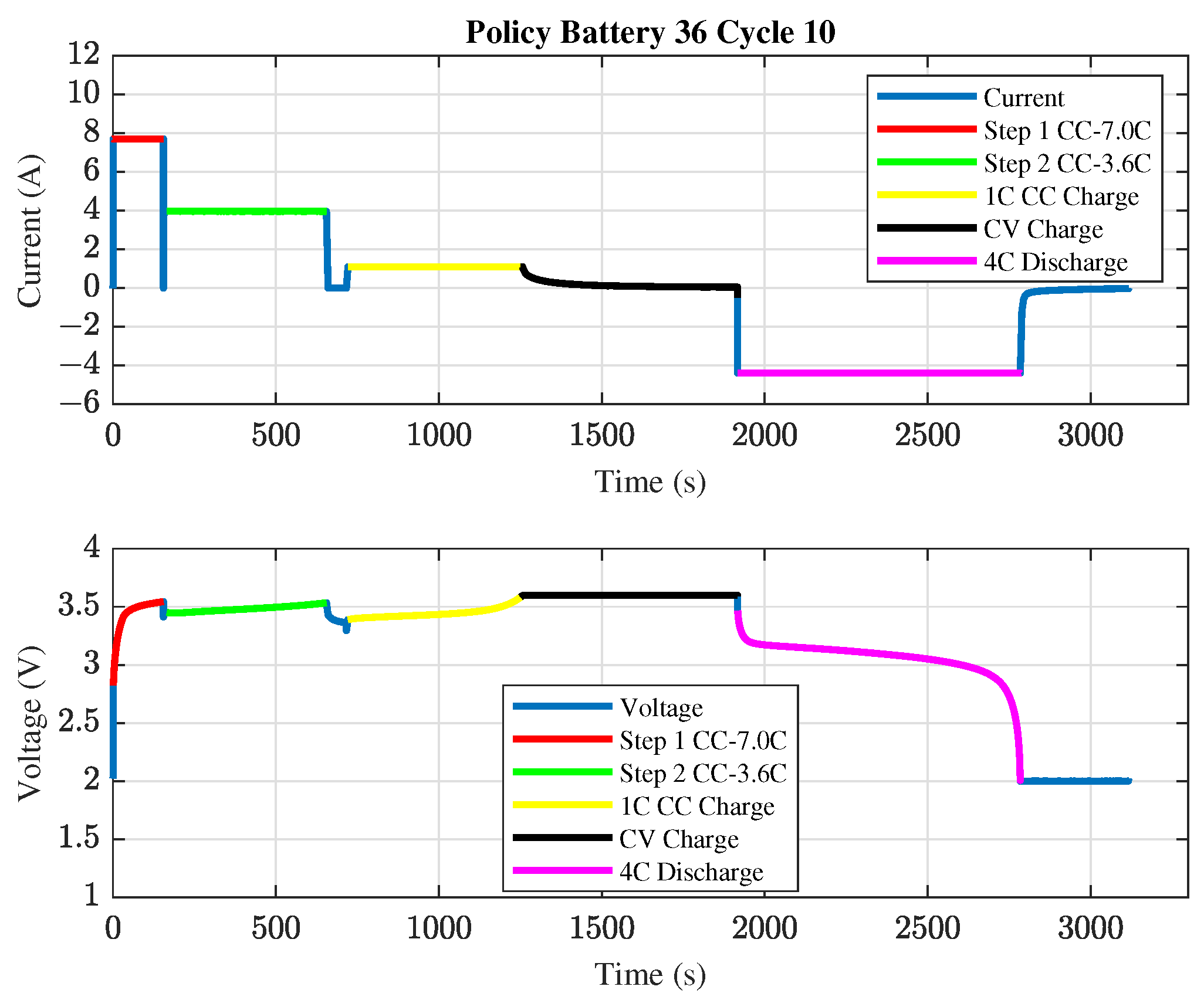
The batteries were cycled while placed in a forced convection temperature chamber set to 30 °C. An example of a typical cycle is shown in Figure 1 (the example refers to battery #36). The cycle includes the following phases:
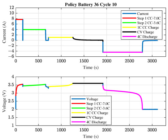
Figure 1.
Example of full charge and discharge cycle for battery #36 of the dataset.
- 1.
- Fast charge including one or more current steps (red and green steps in Figure 1);
- 2.
- Rest phase, lasting between 5 and 5 , depending on the cell;
- 3.
- 1C CC charging up to , followed by a CV stage, ending when the current reaches the low current threshold of C/50 or C/20 depending on the battery;
- 4.
- Discharge at 4C down to the lower cutoff voltage;
- 5.
- Rest phase before the next cycle, with durations between 1 and 5 , depending on the cell.
Each battery has assigned a cycling policy described by a string with the format:
Here, the three fields define the experiment fast charging stage of the cycle for each battery. In a first step, the CC value is used to charge the battery up to the SoC value , which is expressed as a percentage. The second CC step current brings the battery up to 80% SoC. The values for and are formatted as x_d, where x is the integer part and d is the fractional part.
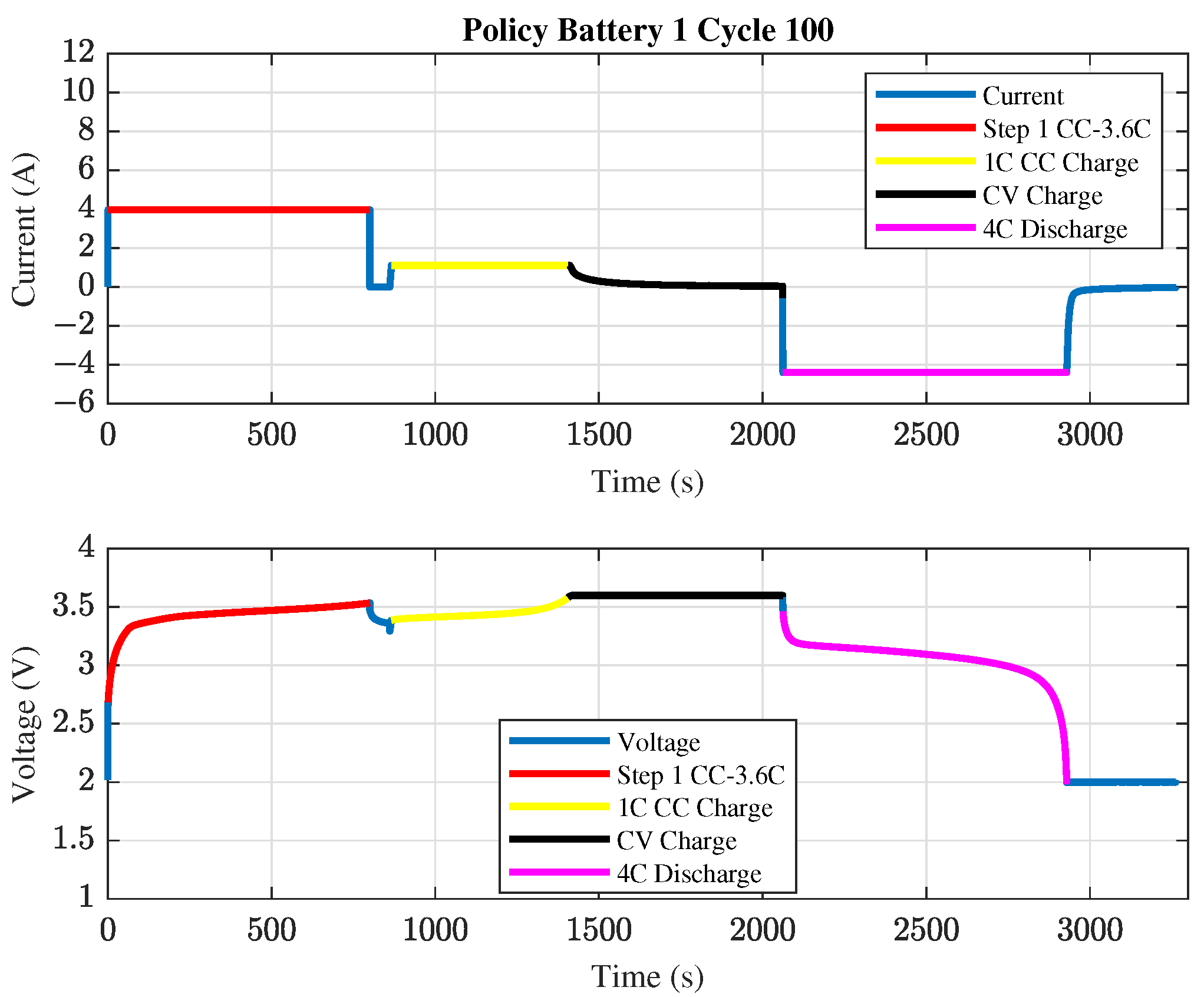
Figure 1 shows an example of the charging and discharging cycles for battery 36, which has a 7C-30PER_3_6C policy. Considering the string defining the policy, the cycle is characterized by a first step current at 7C up to 30% SoC and a second step current at 3.6C up to 80% SoC. In the case of policies with a single fast charging step, is set equal to , and %. Figure 2 shows a typical cycle for battery #1, which is characterized by a single fast charging step of 3.6C up to 80% SoC (3_6C-80PER_3_6C).
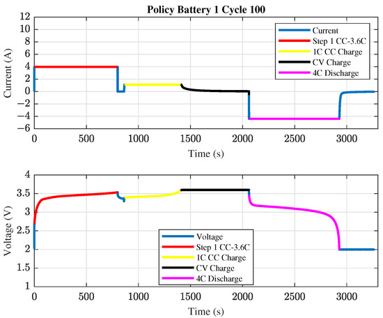
Figure 2.
Example of full charge and discharge cycle for battery #1 of the dataset.
The dataset is divided into three “batches” of 46, 48, 46 sets of data each. In this work, we use the first two batches only, for a total of 89 batteries, because they include tests for which it is possible to obtain the main peak of the IC curves. The analyzed 89 batteries were cycled under 63 different fast-charging policies, with first-step currents from 1C to 8C and second-step currents from 3C to 6C. The batteries have a widely varying cycle life ranging from 148 to 2238 cycles.
In order to analyze the aging trends in the dataset, it is worthwhile to group batteries characterized by similar cycling conditions. Therefore, we divide the 89 batteries into 15 groups with similar fast charging policies. The groups labeled 1, 2 and 3 have a one-step charging policy, whose current increases with the group ID. The other groups have a two-step charging policy with a first-step current that grows with group ID. The batteries in groups 1, 8, 9, 11, 12 and 15 are characterized by equal values for both and ; for groups 7, 10, 13 and 14, is the same within each group, while varies. The remaining groups collect the remaining batteries (2–6). Table 1 collects all the information about the batteries grouping considered in this work.

Table 1.
Considered batteries groups defined according to fast charging policy.
3. Incremental Capacity Main Peak Area Extraction
We evaluate the high-current IC for the 89 batteries belonging to the first two batches of the dataset according to the procedure described in detail by Ospina Agudelo et al. in [13]. In particular, we extract the main peak features, namely its position, height and area, from the 1C CC charging stage. For the available dataset, such a stage always starts when the battery reaches 80% SoC. In practice, the initial SoC value may be selected according to the application, depending on the battery technology and usage patterns.
As discussed in [13], by definition, the main peak area, , can be interpreted as a partial capacity related to the full capacity, meaning that it can be used as capacity indicator regardless of the initial SoC value as long as the employed value is kept constant between computations. The procedure for extraction can be summarized in the following main steps:
- Extraction of current and voltage data during a CC charge stage;
- Filtering of the voltage data using a Savitzky–Golay (SG) approach, leading to the filtered voltage ;
- Computation of the capacity q through integration with a trapezoidal approximation;
- Computation of the incremental capacity ():where k is the discrete time step;
- Application of a Gaussian-Weighted Moving Average filter (GWMA) to to obtain ;
- Extraction of peak position (), peak height (), and in a voltage window , as illustrated by Figure 3, which shows an example of an IC curve filtered by the GWMA filter.
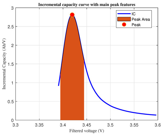 Figure 3. Incremental capacity curve sample with main peak features highlighted.
The selection of the SG filter for the voltage signal over other moving window filters was motivated by its capability to preserve the location of interest points of the curve [26]. Similarly, for the filtering of the data, the GWMA gave better performance than simpler alternatives, such as the moving average or SG filters. With a suitable tuning of the filter window, the GWMA filter reaches desirable smoothing levels with very low distortion of the IC curve features. The higher performance of this filter compared to other approaches is confirmed by Li et al. for low-current IC [27].
The filters parameters have been adjusted for the dataset. The window of the SG filter is set equal to five samples, the window for the GWMA filter is 20 , and . The value of was selected empirically by aiming to maximize the correlation between and SoH while avoiding that the voltage range used for the area computation falls outside of the available voltage data points. Furthermore, it is worth highlighting that the use of a fixed during the whole battery first life aims to enable the computation even when the data for the whole peak is not available.
4. Models for Capacity Estimation from the Incremental Capacity Main Peak Area
The procedure described in Section 3 is applied to all the available cycles for the 89 batteries. It is worth mentioning that some cycles are affected by errors in the acquisition, such as missing portions of data, and were not processed for IC curve extraction in order to avoid unnecessary outlier points. After the removal of the irregular cycles, the discharge capacity Q of the battery, computed in the 4C-discharge phase, can be related, cycle by cycle for each battery, to the IC peak area . It is worth noting that the computation of Q through a 4C CC discharge current, which is the only one available in all tests, leads to lower capacity values than those expected using typical characterization currents, such as 1C or C/20. Nevertheless, despite the underestimation, we expect that the conclusions obtained for this scenario, regarding the relation, hold for typical characterization cases.
A visual inspection of the scatter plots for the batteries first life allowed us to identify two potential sets of cells: batteries with linear and non-linear relationships. In order to evaluate which model is suitable for each battery, we perform a regression analysis on all the first life data available for each battery. We consider one linear model and three non-linear models.
The first model considered is a linear equation:
where and are the fitting coefficients representing, respectively, the slope and intercept of the model. An example of a scatter plot for a battery in the linear set is presented in Figure 4, which also includes the fitted linear model.
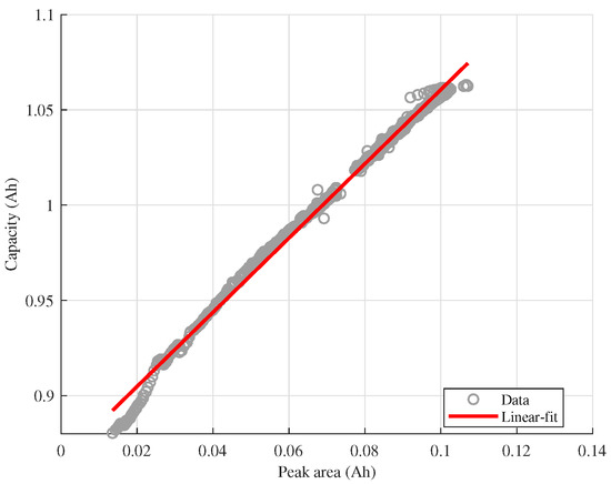
Figure 4.
Example of linear (solid line) model fitting for battery #18 first life data (markers).
For the batteries with a clear non-linear relationship, three additional models were considered, starting with a second-degree polynomial function:
where , and are the model coefficients. The third model is characterized by a power law:
with fitting parameters , , and . Finally, the shape of the aging curve suggests to consider also a logarithmic model:
The model is again characterized by two fitting coefficients, and .
Figure 5 shows an example of the performance of the four fitting models for battery #42. In this case, as well as for the other batteries in the non-linear set, the power law model has on average the best fitting performance in terms of Root Mean Squared Error (RMSE).
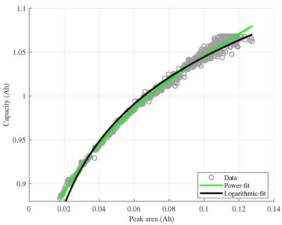
Figure 5.
Example of power law and logarithmic (solid line) models fitting for battery #42 first life data (markers).
We compute the fitting coefficients for each battery in Matlab by using the built-in function fit. The function gives as output the fitting coefficients of the models, the square of the correlation coefficient , and the RMSE. In order to summarize the obtained results, we computed the mean and the standard deviation over all the batteries of the models coefficients, and RMSE. The aggregated results are presented in Table 2.

Table 2.
Average values and standard deviations of the parameters of the linear, polynomial, power and logarithmic models for all 89 batteries.
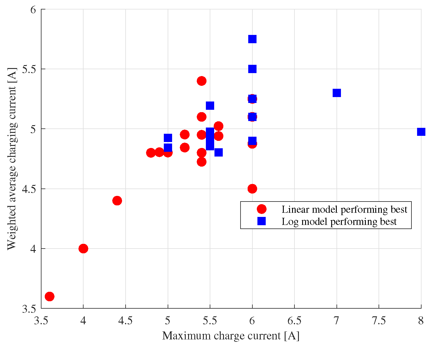
The average is satisfactorily high for all the models, with the polynomial and power law models having the highest averages over all the batteries. The power law model is also characterized by the lowest average RMSE (less than ). Unfortunately, its coefficients deeply vary among batteries, as shown by the highest values of standard deviation for the fitting coefficients (overtaking 45%). Such values indicate that the parameter values are strongly dispersed, and this model has poor generalization capabilities when considering varied aging policies. Conversely, the logarithmic model has good values for and RMSE, and, in addition, the values of the standard deviations for and are low. This result suggests using the logarithmic model to represent the link when the linear model is not enough. After an analysis of the obtained values per battery, we divided the batteries into two sets: Set A including all the batteries from groups with a majority of cases with an value for the linear model higher than the one for the logarithmic model and Set B for the batteries from the remaining groups. In order to identify if there is any relation between the fast charging policy parameters and which is the model with the highest for each battery, we checked the distribution of the batteries for which the logarithmic and linear models gave the best performance in terms of the fast charging stage characteristics. This is summarized in Figure 6, where we plot the maximum fast charging current (namely ) against the weighted average fast charging current, which is computed as:
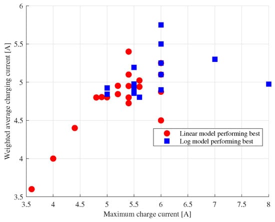
Figure 6.
Maximum and weighted current during fast charging for the batteries with a difference in higher than 1%.
The points in the plot in Figure 6 represent the batteries with a difference over 1% between the values for the linear and logarithmic models, with the circles corresponding to batteries better represented by the linear model and the squares the batteries with higher for the logarithmic model. The distribution of the points in the plain highlights that batteries with lower maximum and average currents can be better represented using a linear relationship, while for the cases with higher maximum currents, the non-linearity of the capacity fading leads to a relation better represented by the logarithmic model.
5. Fitting Results on Battery Groups
In order to further evaluate the generalization capabilities of the models for Sets A and B, we perform fits of the linear and logarithmic models per group introduced in Table 1. For each group, the fitted data include the first-life data of all batteries.
Table 3 shows the results of the linear and logarithmic fits for each battery group, including the models coefficients, and RMSE. Additionally, Table 3 also presents the average and standard deviation of each quantity. On average, over all the groups, values over and RMSE values under were obtained for both models, showing the suitability of both models for representing the relationship between Q and for multiple batteries cycled under similar fast charging regimes.

Table 3.
Values of , , , , , and RMSE () for the linear and logarithmic models computed for the 15 groups.
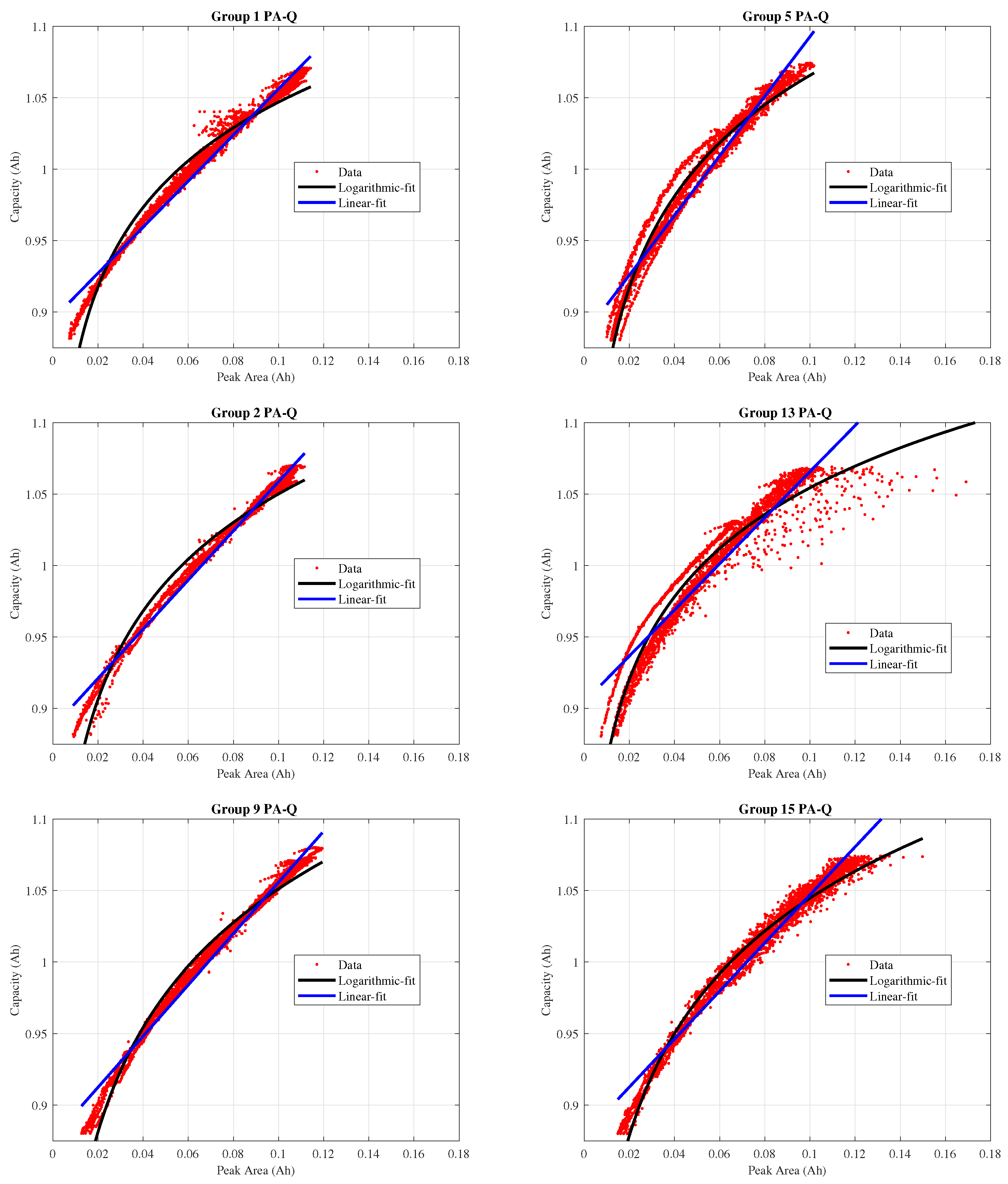
As expected, the logarithmic performs better for groups 4, 5, 13, 14 and 15, which include most of the batteries identified in the previous section as having a non-linear relationship. In particular, increases over 1% in terms of with respect to the linear model can be observed for groups 5, 13 and 15, which is further evidenced by the scatter plots in the right side of Figure 7, where it can be observed how the logarithmic model is better at following the non-linear tendency of said battery groups. For the remaining groups, the linear model seems to be enough for characterizing the relation during the first life, as it was previously identified for batteries aged using non-fast-charging patterns [13]. It is worth mentioning that during the first life, the linear model seems to have the best fitting performance when the considered batteries were aged with a single step fast charging policy at relatively low current values, as evidenced by the results for groups 1 and 2, as presented in the left side of Figure 7.
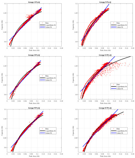
Figure 7.
Capacity Q as a function of the peak area for various battery groups.
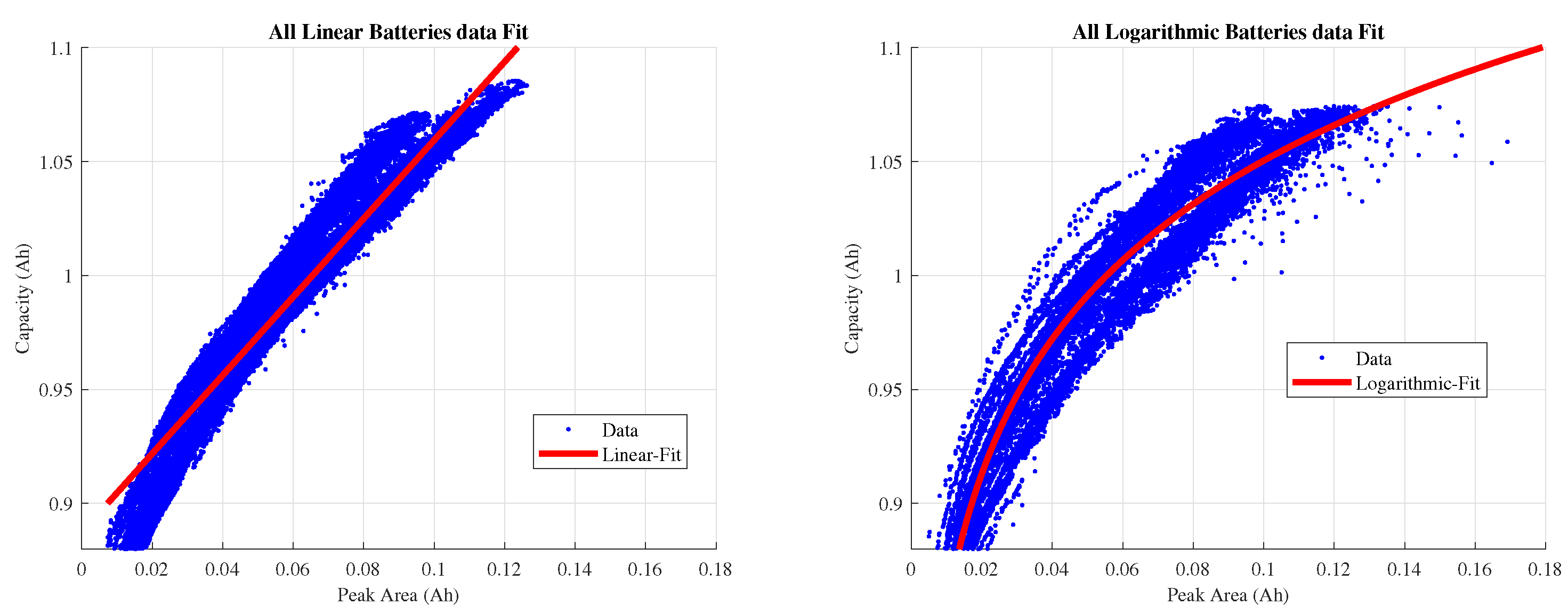
As a final evaluation of the generalization capabilities of the linear and logarithmic models during the first life of batteries, we performed a single fit per batteries set and evaluated their and RMSE. The results for the linear and logarithmic models fitted using the data from Set A and Set B, respectively, are presented in Figure 8.

Figure 8.
Linear (left) and logarithmic (right) models applied to all the first-life data of Set A and Set B.
Even with the considerable dispersion in the datapoints available for the batteries identified as following a logarithmic tendency, for both sets, values over 0.9 were found as presented in Table 4. With RMSE values of % and % for the linear and logarithmic models, respectively, over the available first-life datapoints, we can conclude that the models are suitable for representing the relationship even when profiles with vastly different fast-charging current values are considered.

Table 4.
Values of , , , and RMSE calculated for calculated for all batteries in Set A and values of , , , and RMSE for all batteries in Set B.
6. Peak Area-Based Models for Battery Capacity Prediction
In Section 4, the inference analysis of battery data showed that the linear and logarithmic models (2) and (5) are the most suitable for the representation of the relationship for batteries Set A (groups 1, 2, 3, 6, 7, 8, 9, 10, 11 and 12) and Set B (groups 4, 5, 13, 14 and 15), respectively. In this section, we move from inference to prediction using the same models. We emulate a scenario in which the models are initially trained on a given set of batteries, which is called the training set. Then, we use the trained models to predict the battery capacity on another set, namely the test set, evaluating the forecasting performance of such models.
We implemented the aforementioned scenario by dividing both Set A and Set B into two parts each. The first part, employed as a training set, is used to estimate the coefficients for the linear and logarithmic models using ordinary least squares. The other part of the set is used for the evaluation of the prediction performance in terms of Mean Squared Error (MSE). We take into consideration that each set contains multiple groups of batteries, containing from three to eight batteries each. Therefore, the data split focuses on each group. For each group in each set, 70% of the batteries are randomly selected, and their data are added to the training set. Conversely, the data of the remaining batteries are added to the test set.
6.1. Prediction on Battery First Life
The first prediction analysis is performed only on the first-life data available for each battery. For Sets A and B, the model fitting and evaluation procedures were performed for 10,000 random splits of batteries. For all the trained models, we collected the MSE values achieved in each test and compute their average and standard deviation , as summarized by the upper half of Table 5.

Table 5.
Prediction average results for 10,000 random splits of data.
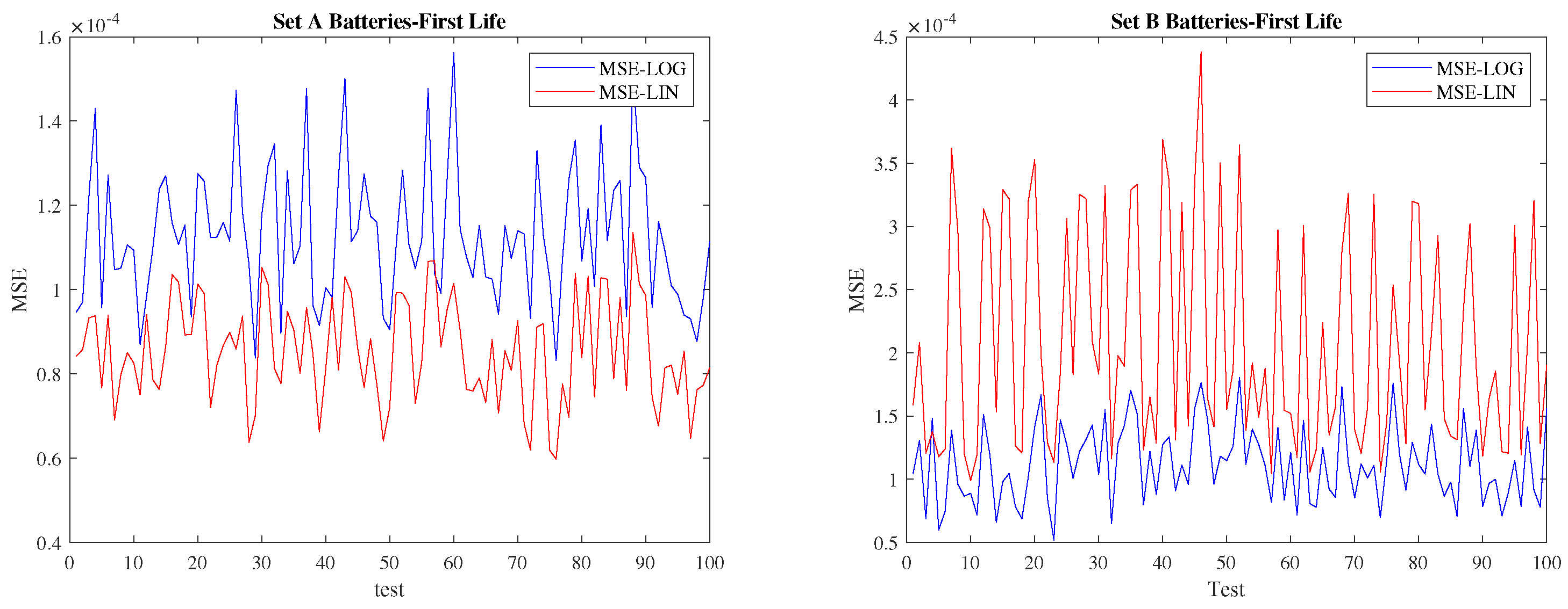
As expected, the linear model shows a lower over all the tests for Set A, with a decrease of % with respect to the logarithmic model. The opposite is true for Set B, for which the logarithmic model introduced a reduction of % in the when compared with the linear model. These results are in full agreement with the inference analysis of Section 5. Figure 9 graphically represents the results in terms of MSE for the first 100 prediction tests.
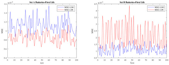
Figure 9.
First life prediction results for 100 random splits of data test.
The right-hand side plot in the Figure 9 highlights multiple spikes in the MSE plot for the linear model, corresponding to cases on which batteries with higher current values during fast charging are left only on the test set, leading to high errors. The logarithmic model shows a considerably lower dependency of MSE on the battery split, highlighting its suitability as a global model.
6.2. Prediction beyond First Life
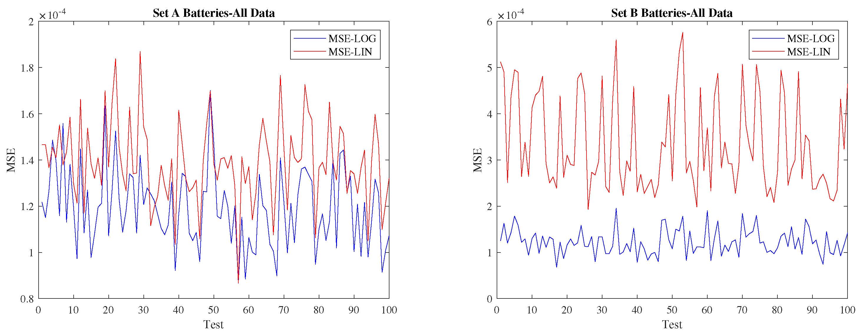
The prediction results beyond the first life of the batteries are shown in the bottom of Table 5 and in Figure 10. It is worth noticing that these results of the predictions change here with respect to those presented above. Here, the logarithmic model has the lowest MSE for the majority of the data splits. On the one hand, for the batteries in Set A, where all batteries go beyond the first life, the very well-known “elbow” effect appears. Obviously, such an effect can better be represented by the logarithmic model, even if the improvement introduced by this model is of only % with respect to the linear model, as shown in the left-hand side plot of Figure 10. The right-hand side plot clearly shows that the logarithmic model is much more accurate for batteries in Set B. The improvement is larger than the one achieved from first-life prediction.
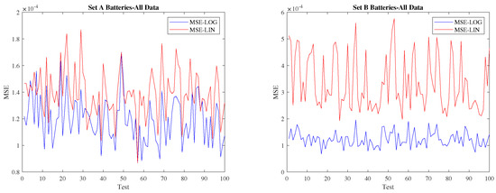
Figure 10.
Full-life prediction results for 100 random splits of data test.
These results show that the logarithmic model is of high interest when considering battery capacity estimation beyond the typical first-life threshold. We believe that it can be considered a promising global modeling approach to battery aging in a framework with fast charging and extended life.
7. Conclusions
The Incremental Capacity (IC) analysis applied to the batteries in the Toyota fast charging dataset shows that the peak area of the IC curves is a viable indicator to estimate the 4C discharge capacity Q and state-of-health for batteries cycled with fast charging profiles. During a fitting analysis performed over individual batteries subject to multistep fast charging profiles during first life, we identified that batteries with maximum and average fast charging currents under 5 showed a linear , which is in agreement with previous results considering usage patterns without fast charging.
When employing higher currents, both maximum and on average, the relationship may exhibit non-linear tendencies, which can accurately be represented by a logarithmic model. Logarithmic representations were favored over other non-linear alternatives, as the fitting results obtained with the logarithmic models lead to lower standard deviations in the adjusted model coefficients. Those results were confirmed for battery groups with similar fast charging policies, showing the generalization capabilities of the models.
Then, batteries were classified into two sets: those for which the linear model performed better during the inference analysis, and the remaining ones, namely Sets A and B. The performance on a prediction framework of the linear and logarithmic models was evaluated by adopting a cross-validation approach. For each set, we adopted a 70–30% training–test split of batteries. The training and test procedure was repeated 10,000 times for each set. As expected, the linear model presented a lower average MSE over all the tests for Set A, with a decrease of 24.35% with respect to the logarithmic model. The opposite is true for Set B, for which the logarithmic model introduced a reduction of 44.73% in terms of average MSE when compared with the linear model. These results change when extending the prediction analysis beyond the first life of the batteries; in such a case, the logarithmic model has the lowest MSE for the majority of the data splits. On the one hand, for the batteries in Set A, going beyond first life leads to the appearance of the very well-known “elbow” effect, which can be better represented by the logarithmic model. On the other hand, the inclusion of data points beyond the first life further improves the logarithmic model performance for batteries in Set B. These results show that the logarithmic model is of great interest for battery capacity estimation beyond the typical first-life threshold.
Author Contributions
Conceptualization, L.L., B.O.A. and W.Z.; methodology, L.L., B.O.A. and W.Z.; software, L.L.; validation, L.L. and B.O.A.; formal analysis, L.L. and B.O.A.; investigation, L.L., B.O.A. and W.Z.; resources, W.Z. and E.M.; data curation, L.L. and B.O.A.; writing—original draft preparation, L.L., B.O.A. and W.Z.; writing—review and editing, L.L., B.O.A., W.Z. and E.M.; visualization, L.L.; supervision, W.Z. and E.M.; project administration, W.Z. and E.M.; funding acquisition, W.Z. and E.M. All authors have read and agreed to the published version of the manuscript.
Funding
The work was supported in part by funds of the projects “Holistic approach to EneRgy-efficient smart nanOGRIDS—HEROGRIDS” (PRIN 2017 2017WA5ZT3) within the Italian MUR 2017 PRIN program, FARB funds of the University of Salerno, and by funds of a public grant overseen by the French National Research Agency (ANR) as part of the “Investissements d’Avenir” program (reference: ANR-16-IDEX-0008).
Data Availability Statement
Not applicable.
Conflicts of Interest
The authors declare no conflict of interest.
Abbreviations
The following abbreviations are used in this manuscript:
| CC | Constant Current |
| CV | Constant Voltage |
| DV | Differential Voltage |
| EV | Electric Vehicle |
| GPR | Gaussian Process Regression |
| GWMA | Gaussian-Weighted Moving Average |
| HCIC | High-Current Incremental Capacity |
| IC | Incremental Capacity |
| LFP | Lithium Iron Phosphate |
| MSE | Mean Squared Error |
| RMSE | Root Mean Squared Error |
| SG | Savitzky–Golay |
| SoC | State of Charge |
| SoH | State of Health |
References
- Stockkamp, C.; Schäfer, J.; Millemann, J.A.; Heidenreich, S. Identifying Factors Associated with Consumers’ Adoption of e-Mobility—A Systematic Literature Review. Sustainability 2021, 13, 10975. [Google Scholar] [CrossRef]
- Keil, P.; Jossen, A. Charging protocols for lithium-ion batteries and their impact on cycle life—An experimental study with different 18650 high-power cells. J. Energy Storage 2016, 6, 125–141. [Google Scholar] [CrossRef]
- Mathieu, R.; Briat, O.; Gyan, P.; Vinassa, J.M. Electro-Thermal Behavior of Four Fast Charging Protocols for a Lithium-Ion Cell at Different Temperatures. In Proceedings of the IECON 2018—44th Annual Conference of the IEEE Industrial Electronics Society, Washington, DC, USA, 21–23 October 2018; pp. 1777–1782. [Google Scholar] [CrossRef]
- Epding, B.; Rumberg, B.; Mense, M.; Jahnke, H.; Kwade, A. Aging-Optimized Fast Charging of Lithium Ion Cells Based on Three-Electrode Cell Measurements. Energy Technol. 2020, 8, 2000457. [Google Scholar] [CrossRef]
- Mathieu, R.; Briat, O.; Gyan, P.; Vinassa, J.M. Comparison of the impact of fast charging on the cycle life of three lithium-ion cells under several parameters of charge protocol and temperatures. Appl. Energy 2021, 283, 116344. [Google Scholar] [CrossRef]
- Noura, N.; Boulon, L.; Jemeï, S. A Review of Battery State of Health Estimation Methods: Hybrid Electric Vehicle Challenges. World Electr. Veh. J. 2020, 11, 66. [Google Scholar] [CrossRef]
- Park, S.; Ahn, J.; Kang, T.; Park, S.; Kim, Y.; Cho, I.; Kim, J. Review of state-of-the-art battery state estimation technologies for battery management systems of stationary energy storage systems. J. Power Electron. 2020, 20, 1526–1540. [Google Scholar] [CrossRef]
- Lin, C.; Xu, J.; Shi, M.; Mei, X. Constant current charging time based fast state-of-health estimation for lithium-ion batteries. Energy 2022, 247, 123556. [Google Scholar] [CrossRef]
- Yang, J.; Cai, Y.; Mi, C. Lithium-ion battery capacity estimation based on battery surface temperature change under constant-current charge scenario. Energy 2022, 241, 122879. [Google Scholar] [CrossRef]
- Li, K.; Zhou, P.; Lu, Y.; Han, X.; Li, X.; Zheng, Y. Battery life estimation based on cloud data for electric vehicles. J. Power Sources 2020, 468, 228192. [Google Scholar] [CrossRef]
- Tan, X.; Tan, Y.; Zhan, D.; Yu, Z.; Fan, Y.; Qiu, J.; Li, J. Real-Time State-of-Health Estimation of Lithium-Ion Batteries Based on the Equivalent Internal Resistance. IEEE Access 2020, 8, 56811–56822. [Google Scholar] [CrossRef]
- Jenu, S.; Hentunen, A.; Haavisto, J.; Pihlatie, M. State of health estimation of cycle aged large format lithium-ion cells based on partial charging. J. Energy Storage 2022, 46, 103855. [Google Scholar] [CrossRef]
- Ospina Agudelo, B.; Zamboni, W.; Monmasson, E. Application domain extension of incremental capacity-based battery SoH indicators. Energy 2021, 234, 121224. [Google Scholar] [CrossRef]
- Zhang, Y.; Liu, Y.; Wang, J.; Zhang, T. State-of-health estimation for lithium-ion batteries by combining model-based incremental capacity analysis with support vector regression. Energy 2022, 239, 121986. [Google Scholar] [CrossRef]
- Riviere, E.; Sari, A.; Venet, P.; Meniere, F.; Bultel, Y. Innovative incremental capacity analysis implementation for c/lifepo 4 cell state-of-health estimation in electrical vehicles. Batteries 2019, 5, 37. [Google Scholar] [CrossRef]
- Fly, A.; Chen, R. Rate dependency of incremental capacity analysis (dQ/dV) as a diagnostic tool for lithium-ion batteries. J. Energy Storage 2020, 29, 101329. [Google Scholar] [CrossRef]
- Riviere, E.; Venet, P.; Sari, A.; Meniere, F.; Bultel, Y. LiFePO4 Battery State of Health Online Estimation Using Electric Vehicle Embedded Incremental Capacity Analysis. In Proceedings of the 2015 IEEE Vehicle Power and Propulsion Conference, VPPC 2015 Proceedings, Montreal, QC, Canada, 19–22 October 2015. [Google Scholar] [CrossRef]
- Tang, X.; Zou, C.; Yao, K.; Chen, G.; Liu, B.; He, Z.; Gao, F. A fast estimation algorithm for lithium-ion battery state of health. J. Power Sources 2018, 396, 453–458. [Google Scholar] [CrossRef]
- Tang, J.; Liu, Q.; Liu, S.; Xie, X.; Zhou, J.; Li, Z. A Health Monitoring Method Based on Multiple Indicators to Eliminate Influences of Estimation Dispersion for Lithium-Ion Batteries. IEEE Access 2019, 7, 122302–122314. [Google Scholar] [CrossRef]
- Li, X.; Yuan, C.; Li, X.; Wang, Z. State of health estimation for Li-Ion battery using incremental capacity analysis and Gaussian process regression. Energy 2020, 190, 116467. [Google Scholar] [CrossRef]
- Li, X.; Yuan, C.; Wang, Z. State of health estimation for Li-ion battery via partial incremental capacity analysis based on support vector regression. Energy 2020, 203, 117852. [Google Scholar] [CrossRef]
- Zheng, L.; Zhu, J.; Lu, D.D.C.; Wang, G.; He, T. Incremental capacity analysis and differential voltage analysis based state of charge and capacity estimation for lithium-ion batteries. Energy 2018, 150, 759–769. [Google Scholar] [CrossRef]
- Ospina Agudelo, B.; Zamboni, W.; Postiglione, F.; Monmasson, E. Battery State-of-Health estimation based on multiple charge and discharge features. Energy 2023, 263, 125637. [Google Scholar] [CrossRef]
- Severson, K.A.; Attia, P.M.; Jin, N.; Perkins, N.; Jiang, B.; Yang, Z.; Chen, M.H.; Aykol, M.; Herring, P.K.; Fraggedakis, D.; et al. Data-driven prediction of battery cycle life before capacity degradation. Nat. Energy 2019, 4, 383–391. [Google Scholar] [CrossRef]
- Severson, K.A.; Attia, P.M.; Jin, N.; Perkins, N.; Jiang, B.; Yang, Z.; Chen, M.H.; Aykol, M.; Herring, P.K.; Fraggedakis, D.; et al. Data-Driven Prediction of Battery Cycle Life before Capacity Degradation—Dataset. Toyota Res. Inst. 2019. Available online: https://data.matr.io/1/projects/5c48dd2bc625d700019f3204 (accessed on 1 December 2022).
- Schafer, R.W. What Is a Savitzky-Golay Filter? Lecture Notes. IEEE Signal Process. Mag. 2011, 28, 111–117. [Google Scholar] [CrossRef]
- Li, Y.; Abdel-Monem, M.; Gopalakrishnan, R.; Berecibar, M.; Nanini-Maury, E.; Omar, N.; van den Bossche, P.; Van Mierlo, J. A quick on-line state of health estimation method for Li-ion battery with incremental capacity curves processed by Gaussian filter. J. Power Sources 2018, 373, 40–53. [Google Scholar] [CrossRef]
Disclaimer/Publisher’s Note: The statements, opinions and data contained in all publications are solely those of the individual author(s) and contributor(s) and not of MDPI and/or the editor(s). MDPI and/or the editor(s) disclaim responsibility for any injury to people or property resulting from any ideas, methods, instructions or products referred to in the content. |
© 2022 by the authors. Licensee MDPI, Basel, Switzerland. This article is an open access article distributed under the terms and conditions of the Creative Commons Attribution (CC BY) license (https://creativecommons.org/licenses/by/4.0/).

