An Incremental Capacity Parametric Model Based on Logistic Equations for Battery State Estimation and Monitoring

Abstract

An incremental capacity parametric model for batteries is proposed. The model is based on Verhulst’s logistic equations and distributions in order to describe incremental capacity peaks. The model performance is compared with polynomial models and is demonstrated on a commercial lithium-ion cell. Experimental data features low-current discharges performed at temperatures ranging from −20 °C to 55 °C. The results demonstrate several advantages of the model compared to empirical models. The proposed model enables a clear description of the geometric features of incremental capacity peaks. It also doubles as an open circuit voltage model as the voltage curve can be fully recovered from parameterization on incremental capacity curves. The study of temperature sensitivity show that peak geometric parameters can be modelled as a function of temperature. An example of practical application is then displayed by using the model to estimate battery state-of-charge from voltage and temperature measurements. This example can expand to other practical applications for battery management systems such as state-of-health monitoring.

1. Introduction

Lithium-ion batteries are widely used in a variety of applications ranging from small portable electronics to multi-kWh systems such as electric vehicles (EVs) or grid energy storage. To ensure safety, operability, and long lifetime of the batteries, a battery management system (BMS) is integrated with the battery pack. A BMS can be made of a single system connected to each cell in the pack or it can be split into a master controller and multiple slave modules [1]. It generally fulfills three tasks: acquisition, estimation, and control [2]. Acquisition consists of measuring voltage, current and temperature of either the pack or subparts of the pack, down to the cell. The purpose of estimation is to evaluate both the state-of-charge (SoC) and the state-of-health (SoH) of each individual cell, based on cell models and/or algorithms. Control revolves around balancing the cells to avoid SoC disparities which could lead to safety issues or important gaps between batteries SoHs. This control is generally optimized to meet specific requirements for the application, meaning the estimation method will be responsible for how well the battery pack performs and lasts.

SoC estimation in BMS directly relies on cell voltage measurements jointly with algorithms based on a model of the cell electrical behavior [3,4]. The voltage of a lithium-ion cell is comprised of two parts. The first part has a thermodynamic origin and is called the open-circuit voltage (OCV), which is the voltage in steady-state. The second part has a kinetic part, which consists of overvoltage caused by internal phenomena in the cell [5]. The models used for SoC estimation thus contain these two parts, whether they can be classified as electrochemical models (physical, close to first principles) [6], equivalent circuit model (electrical, empirical) [7], or data-driven (statistical, black-box) [8]. Moreover, it has been a recent trend to couple these different methods for improved results such as physics-based equivalent circuit models [9] and physics-informed data-driven methods [10]. The rest of this article focuses on the OCV part of the cell voltage.

The OCV can be obtained through cell voltage measurements by either waiting for the steady-state, mathematically subtracting the influence of the voltage relaxation [11], or approximating it by performing low-current current charge or discharge to approach the steady-state [12]. The OCV primarily depends on the cell electrode materials [13]. In addition, the OCV also depends on cell temperature and varies with cell degradation throughout its service life [14]. To summarize, the accuracy of the SoC estimation strongly depends on the accuracy of the OCV model and there have been intense research efforts to improve it. Ideally, the OCV model must be robust and easily adaptable to different cell materials, temperatures, and ageing states.

Several approaches to OCV modelling can be distinguished in the existing literature. Some studies do not aim to mathematically model the OCV. Instead, the experimentally measured OCV is implemented as a lookup table for the cell electrical model [15,16]. The advantages include its simplicity of use and its accuracy, if the lookup table is recorded at a sufficient SoC resolution. However, the OCV also change with temperature and ageing. Especially, taking ageing into account in the lookup table is complex as it cannot be recorded at the beginning of life and several ageing trajectories are possible. Thus, modeling effort can open new opportunities for considering the modification of OCV by temperature and ageing, as it is, in theory, possible to describe the OCV curve with less parameters to be stored, and then to adapt some of these parameters. Other studies propose empirical OCV models, such as those based on polynomials or other usual mathematical functions. Zhang et al. investigated the accuracy of OCV models based on polynomials [17]. Polynomial expressions provide good accuracy and are very adaptable to different electrode chemistries. The main drawback is that these are so distant from OCV physical origin that their parameters lack physical significance when building a multidimensional model, such as demonstrated with sensitivity to temperature in the study of Zhang et al. Apart from polynomials, many examples of empirical models based on different combinations of usual functions have been proposed and can accurately model the OCV curve [4,18,19]. The main obstacle is that such empirical expressions lack adaptability to different electrode chemistries, while also suffering from a lack of physical significance such as for polynomial models. Other studies proposed models closer to the physical origin of OCV by applying thermodynamic principles. Ohzuku and Ueda, as well as Ali, proposed models based on modified Nernst equations [20,21]. However, the models lack accuracy because the OCV does not follow strict Nernstian behavior. To account for this, Karthikeyan et al. developed a model based on the Redlich-Kister equation [22]. The model shows good accuracy for different electrode chemistry. However, the evolution of the numerous parameters with temperature or SoH is not studied. Lavigne et al. proposed a polynomial simplification of the model from Karthikeyan et al. and studied the evolution of model parameters with SoH [23]. Birkl et al. proposed an OCV model based on additive terms of the Fermi–Dirac distribution function [24]. The model shows good accuracy and is adaptable to any Li-ion cell chemistry. However, it features a high number of parameters (24) to adapt to varying temperature or SoH. The main drawback of thermodynamic models is that they often require prior physical knowledge about electrode materials, which makes the model identification more complex.

Interestingly, other studies have proposed modeling the incremental capacity (IC) curve instead of the OCV curve [25,26,27,28]. The IC is the derivative of the capacity with respect to voltage and is thus directly linked to the OCV–SoC relationship. The derivation enables to highlight the phase transitions of electrodes materials, which are plateaus in the OCV curve, as distinguishable peaks in the IC curve. Incremental capacity analysis (ICA) has been widely used in the literature as a way to gain insights into electrode degradation mechanisms and, more generally, as a way to monitor SoH [29,30,31,32,33,34]. In our opinion, modeling the IC curve instead of the OCV curve allows for a direct link between the need for SoC estimation based on OCV and for SoH monitoring based on ICA. The OCV can then be easily recovered by derivation without further need for modeling. An IC model should be both adaptable to different chemistries and robust to different battery states.

In this paper, we thus introduce an IC model for lithium-ion batteries which doubles as an OCV model. The model is based on additive terms of the so-called logistic functions derived from Verhulst’s work [35]. The logistic model provides a good compromise between accuracy and physical meaning. It enables a clear description of the geometric features of IC peaks, and each parameter can be attributed to physical quantities.

This article follows the subsequent structure. Section 2 gives the theoretical background of the proposed incremental capacity model. Section 3 details the experimental methods that were followed to obtain the data. Section 4 analyzes and discusses the results and includes a comparison of the proposed model accuracy with polynomial empirical models, an extension to a multidimensional model by accounting for the effect of temperature, and an example of application of the model for SoC estimation, paving the way for other usages of the model.

2. Incremental Capacity Parametric Model Based on Logistic Equations

This section gathers the theoretical background of the proposed IC model based on Verhulst’s logistic equations.

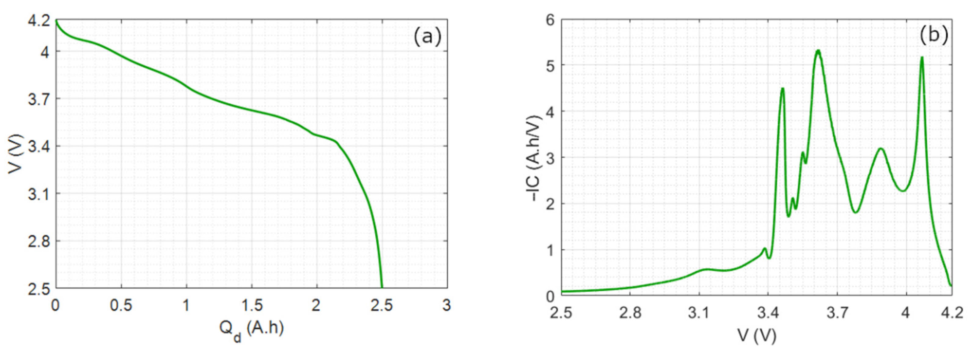
2.1. Open Circuit Voltage and Incremental Capacity

The OCV is the voltage of the cell at a steady state. The cell OCV is the subtraction of the positive electrode open circuit potential (OCP) by that of the negative electrode. Each OCP depends on the concentration of lithium ions in the electrode. On the cell level, the OCV depends on the SoC (the ratio of the amount of capacity left to be discharged on the maximum discharged capacity).

The electrodes OCP display voltage features that are characteristic of the electrode materials and of the chemical phase transitions they undergo in the SoC operating window of the cell [36]. During a bi-phasic transition, the potential of an electrode is independent of the concentration in lithium ions. Hence, the electrode OCP can exhibit potential plateaus. At the cell level, the potential plateaus of each electrode can happen jointly or separately depending on the cell balancing. Thus, the cell OCV displays certain features that depend on the electrode materials and on electrode balancing. Figure 1a provides an example with a low-current discharge to approach the steady-state voltage, represented as a function of the discharged capacity. The voltage curve exhibits features which are characteristic of the cell studied in this paper, comprising a graphite negative electrode and a lithium-nickel-cobalt-aluminum oxide positive electrode (see Section 3 for further details).

As these features are subtle in the voltage curve, it is useful to use derivation to highlight them. For the so-called incremental capacity $IC=f\left(V\right)$, the following derivative is used

$$IC\left(V\right)=\frac{dQ}{dV}\left(V\right),$$

(1)

where $Q$ is the capacity (in A.h), which can either be charged $Q_c$ or discharged $Q_d$, and $V$ is the voltage (in volts). Hence, a plateau in the voltage curve, indicating a transition between two chemical phases, becomes a peak in the IC curve. Figure 1b shows the IC curve corresponding to the previous voltage curve. The peaks at the cell level are convolutions of IC peaks of each electrode [30]. The goal of this article is to develop a general modeling framework of such IC curves, for all battery chemistries and all states.

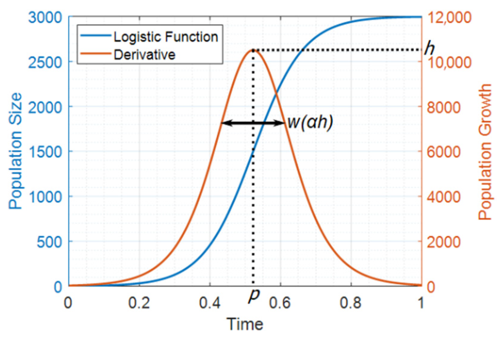
2.2. Verhulst’s Logistic Equations

Historically, P.-F. Verhulst was looking for a human population model accounting for limited resources [35]. In his 1845 publication, he proposed a model based on a differential equation that modifies the Malthusian exponential growth model. The proposed differential equation and all mathematical details are given in Appendix A, while the main equations are kept in the main text. The solution of the proposed differential equation is what P.-F. Verhulst called the logistic equation:

$$y\left(t\right)=\frac{K}{1+\left(\frac{K}{y_0}-1\right)e^{-rt}},$$

(2)

where $y\left(t\right)$ is the population at a given time $t$ and with initial condition $y\left(t=0\right)=y_0$, r is the growth rate, and K the carrying capacity (the maximum population a species can carry given a finite amount of resources). Its derivative is what Verhulst called the logistic distribution and is written as follow

$$\frac{dy}{dt}\left(t\right)=\frac{K\left(\frac{K}{y_0}-1\right)r{e}^{-rt}}{{\left[1+\left(\frac{K}{y_0}-1\right)e^{-rt}\right]}^2}$$

(3)

The logistic Equation (2) and the logistic distribution (3) are represented for a given set of parameters in Figure 2 for illustration purposes. The logistic equation is a case of sigmoid function. It connects asymptotically two parallel segments, defined by the initial population $y_0$ and the maximum population $K$. It has an inflection point which corresponds to a peak for its derivative with symmetry of its left and right side. These geometric properties are used to model IC peaks in the following.

2.3. Incremental Capacity Parametric Model

Each phase transition, corresponding to an IC peak, can be seen as a quantity of the lithium ions exchanged between electrodes as the charge or discharge process occurs. This makes Verhulst’s logistic equation and its derivative particularly fitting, because an analogy between human populations and ions populations can be made. Using this analogy to model the IC curve, population $y$ becomes the capacity $Q$ and time $t$ becomes the voltage $V$.

To model one IC peak, it is more convenient to describe the logistic distribution with its geometric parameters as illustrated on Figure 2. The geometric parameters are its position $p$, its height $h$, and its width $w$ (measured at 94% of the peak’s height, see Appendix A). They can be expressed from $y_0$, $r$, and $K$ (see Appendix A) as follows

$$\{\begin{array}{c}w=\frac{1}{r}\\ h=\frac{Kr}{4}\\ p=\frac{1}{r}\ln \left(\frac{K}{y_0}-1\right)\end{array} .$$

(4)

The logistic Equation (2) and the logistic distribution (3) can then be expressed as functions of $p$, $h$, and $w$, and be simplified by using trigonometric functions (see Appendix A). This process gives the equations that will be used:

$$\{\begin{array}{c}y\left(t\right)=2hw\left[1+\tanh \left(\frac{t-p}{2w}\right)\right]\\ \frac{dy}{dt}\left(t\right)=h{\sec \mathrm{h}}^2\left(\frac{t-p}{2w}\right)\end{array}$$

(5)

In order to accurately model an $IC=f\left(V\right)$ curve such as that shown in Figure 1b, additive terms of the derivative of Equation (5) are used to consider the multiple peaks as expressed in

$$IC\left(V\right)={\displaystyle \sum }_{n=1}^N{h}_n{\sec \mathrm{h}}^2\left(\frac{V-p_n}{2w_n}\right)$$

(6)

where $IC$ is the derivative of $Q_d$ over $V$ (in A.h/V), $N$ is the number of peaks considered, $n$ is the index of each peak, $h_n$ is the height (in A.h/V) of the peak $n$, $p_n$ is the position (in V) of the peak $n$, and $w_n$ is the width (in V) of the peak $n$.

By precisely fitting each peak, it is possible to obtain a matrix of 3 × N parameters, and compute the charged or discharged capacity models $Q=f\left(V\right)$ using additive terms of logistic equations based on Equation (5). As the hyperbolic tangent is a strictly increasing function, the capacity must increase when the voltage increases. Hence, it is the charged capacity $Q_c$ that is expressed as a function of voltage by Equation (7). The discharged capacity $Q_d$ is then easily obtained with Equation (8), where $Q_{d,max}$ is the maximal capacity measured in discharge. The state-of-charge $SoC$ is finally defined by Equation (9).

$$Q_c\left(V\right)={\displaystyle \sum }_{n=1}^{N}2h_n{w}_n\left[1+\tanh \left(\frac{V-p_n}{2w_n}\right)\right]$$

(7)

$$Q_d\left(V\right)=Q_{d,max}-Q_c\left(V\right).$$

(8)

$$SoC\left(V\right)=\frac{Q_{d_{max}}-Q_d\left(V\right)}{Q_{d_{max}}}.$$

(9)

The obtained model $Q=f\left(V\right)$ is equivalent to the model $V=f\left(Q\right)$ or $V=f\left(SoC\right)$. Hence, a model of the OCV curve is obtained in the same process.

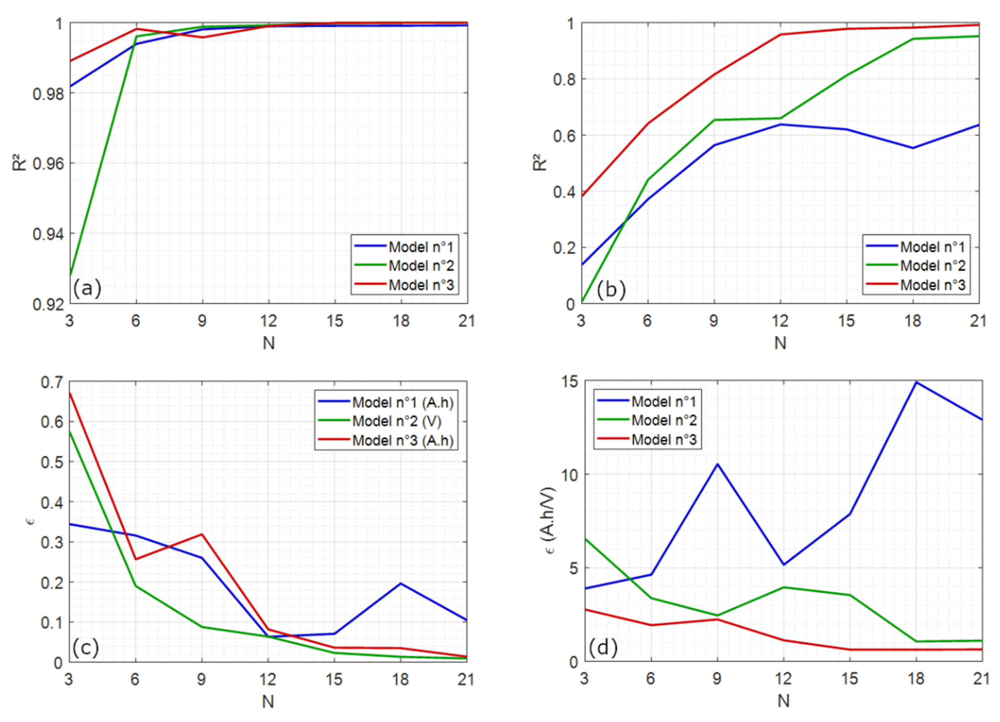
2.4. Comparison with Polynomial Models

In order to demonstrate the performance of the proposed logistic model, it is useful to compare it to a polynomial model.

Generally, polynomial models are defined as a voltage function of SoC, which is particularly useful for equivalent circuit models [17]. However, for SoC estimations, a dedicated SoC (equivalently capacity) function of voltage is required. No general formula exists for finding the roots of polynomials of 5th or more order. As finding the roots is necessary to inverse the polynomial, here, two distinct polynomial models must be defined, one for the SoC (or equivalently capacity), and one for the voltage. The two following models are defined:

$$Q_d\left(V\right)={\displaystyle \sum }_{n=0}^N{a}_n{V}^n$$

(10)

$$V\left(Q_d\right)={\displaystyle \sum }_{n=0}^N{b}_n{Q}_d{}^n,$$

(11)

where $a_n$ (in A.h/V) and $b_n$ (in V/(A.h)) are the polynomials coefficients, $N$ is the order of the polynomial (which thus have $N$ + 1 parameters), and $n$ is the index for each parameters.

3. Experimental Methods

This section gives the experimental details; namely, the characteristics of the lithium-ion cell used and the experimental protocol to gather data to fit the model on.

3.1. Cell Characteristics and Test Equipment

One commercial lithium-ion cell was chosen to perform the experiments. The cell is the Samsung INR18650-25R5 cylindrical 18650. This cell is made of a graphite negative electrode and a LiNi_0.8Al_0.15Co_0.05O₂ (nickel-cobalt-aluminum, NCA) positive electrode. It has a rated nominal capacity of 2.5 A.h, and an operating voltage window between 2.5 V and 4.2 V.

The tests were performed on the Cacyssée platform of the IMS laboratory. All the tests were performed inside a controlled thermal environment with a CLIMATS climatic chamber. Measurements were performed using the 4-wire method and recorded by a BioLogic BCS-815 potentiostat connected to a computer and controlled through the BT-Lab software. Data points were recorded every second.

3.2. Protocol of Experiments

The main goal of the experiments was to obtain low-current discharge data of the graphite/NCA cell in order to numerically derive the incremental capacity curve and parameterize the proposed model. Low-current discharges were preferred to other OCV acquisition methods because it allows us to readily approach the OCV while obtaining many data points, thus enabling numerical derivation [30]. Measurement starts by a 3 h rest for thermal and electrical relaxation. Then, a constant-current–constant-voltage (CC-CV) discharge is performed with a CC current of C/2 (1.25 A) until a cutoff voltage of 2.5 V is reached and maintained in CV stage until the absolute current drops below C/20 (125 mA). Immediately after, a CC charge at C/20 (125 mA) is carried out until a cutoff voltage of 4.2 V. Finally, the low-current discharge is recorded in CC mode at C/20 (125 mA) until a cutoff voltage of 2.5 V. The results constitute the data used in this article. As a side note, the experimental data were obtained by completely charging and discharging the cell at a low current rate to demonstrate a proof-of-concept of the method. In real applications such as electric vehicles, such ideal conditions often cannot be met. However, several methods to accommodate real conditions and recover the IC curves can be employed such as for using partial charging data [37] and using higher current rate [38,39]. Additionally, the OCV hysteresis between charge and discharge that can be observed for certain electrode chemistries [40] was not taken into account in this work for the sake of succinctness. To consider the hysteresis, the low rate discharges could be doubled by low rate charges. Then, the rest of the method should be applied in the same manner, but on charge data.

The other goal of the experiments was to obtain data at different temperatures in order to demonstrate the suitability of the model when a physical dimension is added and its application in accurate SoC estimation at varying temperatures. For this, the previously described low-current discharge test was repeated at different temperature. The tested temperatures were, in order: 55 °C, 40 °C, 25 °C, 10 °C, 0 °C, −10 °C, and −20 °C. The experimental protocol is the same as described in the preceding paragraph, with the temperature change in the thermal chamber being carried out before the 3 h rest starts. It can be remarked that the discharge rate of C/20 gradually becomes a less good approximation of the OCV when the temperature decreases due to kinetic limitations [38]. To improve the OCV approximation, the discharge rate can be reduced, although it was kept constant here for all temperatures to keep the experimental protocol identical.

Incremental capacity data presented in the rest of this article are obtained in the following way. First, high frequency noise on the measured voltage of low-current discharge data is filtered. Then, both the voltage and the capacity derivatives are computed using the gradient function in MATLAB^®. Finally, Equation (1) is used to obtain the IC.

Concerning the procedure used to parameterize the compared models, two different MATLAB^® functions were used. For the proposed logistic model, the function lsqcurvefit is used to solve this nonlinear curve-fitting problem in the least-squares sense. For the two polynomial models, the function polyfit is used to find the best polynomial coefficients, also in the least squares sense.

4. Results and Discussions

The obtained experimental data are used to parameterize the proposed IC model. Before extending the model to a varying temperature, the particular case of 25 °C is studied with a comparison of the proposed model to polynomial models.

4.1. Study of the 25 °C Case

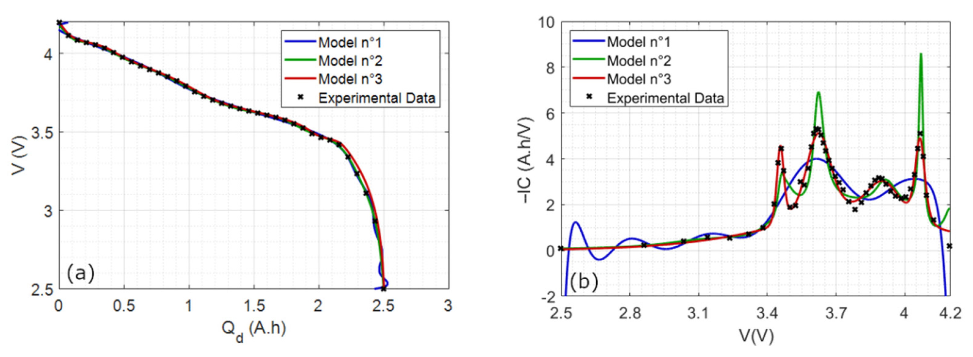
4.1.1. Comparison with Polynomial Models

The models described in Section 2 were fitted to the experimental data. This was carried out for both voltage vs. capacity data and IC vs. voltage data in order to compare the two approaches to modelling the relationship between voltage and capacity (or SoC). In this subsection, “Model n°1” refers to the polynomial $Q=f\left(V\right)$ model of Equation (10), “Model n°2” refers to the polynomial $V=f\left(Q\right)$ model of Equation (11), and “Model n°3” refers to the proposed logistic model either in the form $IC=f\left(V\right)$ of Equation (6) or $Q=f\left(V\right)$ of Equation (7) depending on the current working data.

As the three compared models are adaptative, they do not contain a fixed number of parameters. Hence, a comparison of their accuracy against experimental data as a function of the number of model parameters was first completed. Figure 3 shows the evolution of the coefficient of determination $R^2$ and the root-mean-square error (RMSE) $ϵ$ with the number of parameters for the three compared models and for both voltage vs. capacity data and IC vs. voltage data.

Based on the $R^2$ criterion, the three compared model show a similar good fit to voltage vs. capacity data for $N=6$ or more parameters (Figure 3a). However, the proposed model shows clear superiority when looking at IC vs. voltage data (Figure 3b), with the logistic model being a good fit after only $N=12$ or more parameters, whereas the polynomial models struggle to match these experimental data. Based on the RMSE $ϵ$, the proposed logistic model also shows an advantage. On voltage vs. capacity data, the logistic model performs equivalently to the polynomial model n°2 for $N=12$ or more parameters, while polynomial model n°1 stays a little behind (Figure 3c). On IC vs. voltage data, the logistic model presents a significantly reduced error compared to the polynomial models (Figure 3d), showing clear superiority similar to that observed with $R^2$. It can be noted that the RMSE $ϵ$ and $R^2$ do not show a monotonic evolution with the order of polynomials, contrarily to the logistic model with increasing number of parameters. This behavior is inherent to the nature of polynomial curve-fitting problem, because higher-order polynomials can be oscillatory and lead to a poorer fit to the experimental data points (Mathworks.com, “polyfit, Polynomial curve fitting”. URL = “https://fr.mathworks.com/help/matlab/ref/polyfit.html”, accessed on 7 April 2022).

Based on the results presented in Figure 3, the proposed model shows significative improvements to fit both the capacity and its derivative. This also allows us to determine how many peaks can be kept without significantly reducing the accuracy of the model. For both sets of experimental data and for both fit criteria ($R^2$ and $ϵ$), the logistic model shows already a very good fit to experimental data for $N=15$ parameters, while adding more parameters do not significantly improve the fit. Thus, a number of 15 parameters is selected for the rest of the study. For the proposed model, this means 5 IC peaks are considered for this specific cell. For the polynomial models, this corresponds to a 14th order polynomial.

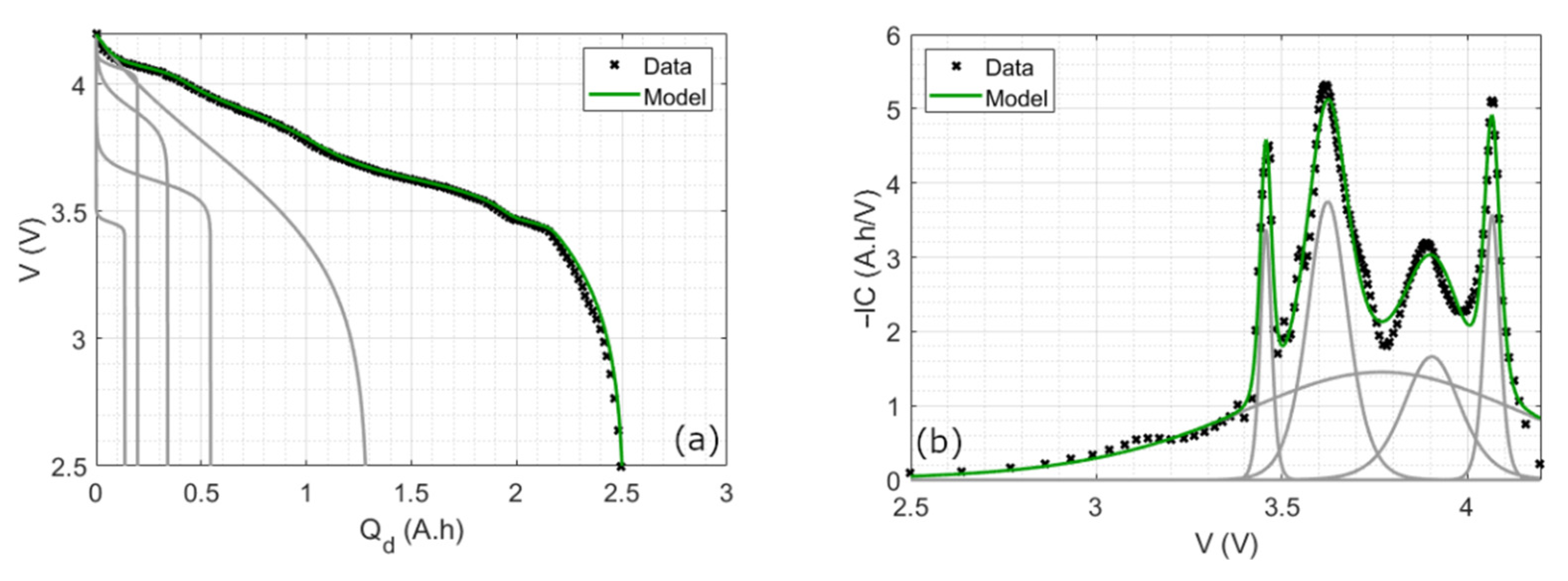
4.1.2. Final Reconstruction

Figure 4 shows the final reconstruction of the proposed logistic model on voltage and incremental capacity curves with $N=15$. It can be seen that the incremental capacity peaks (Figure 4b) are well described by additive terms of the logistic distribution expressed by Equation (6). The incremental capacity curve is thus rebuilt. Each IC peak corresponds to a signature in voltage (Figure 4a), with the multiple contributions adding up to the voltage curve as expressed in Equation (7).

The end of charge and end of discharge points of the OCV are important for calculating the capacity. Here, we can observe that both the whole curve in general, and the endpoints in particular are accurately represented. This is an advantage of fitting the IC curve to recover the OCV: because peaks are geometrically modeled, the accuracy is intrinsically dependent on choosing the right number of peaks for the model. Thus, the method is flexible and would result in a good accuracy for other cell chemistries. Moreover, the method would work similarly on charge data to consider the voltage hysteresis, with the IC peaks in the hysteresis voltage window and corresponding logistic model parameters slightly modified.

With the number of parameters fixed at $N=15$, the fit to experimental data is shown and compared between the three models in Figure 5.

When looking at the whole voltage vs. discharge capacity curve (Figure 5a), the three models show a similar fit to experimental data. However, when looking at the IC curve (Figure 5b), the proposed model demonstrates its advantage compared to the polynomial models. It shows a clear geometric description of IC peaks, which is not the case for polynomials, even at a 14th order.

If the models presented until now fit data in specific conditions (a C/20 discharge at 25 °C on a fresh batterie), the possibility to extend the model to more conditions must be studied. This is carried out in the following way with different temperatures for the logistic model. Because the proposed logistic model has already shown its edge at 25 °C and because polynomials are non-physical, meaning that their parameters do not follow a clear trend with varying temperatures as observed by Zhang et al. [17], polynomial models are not studied further.

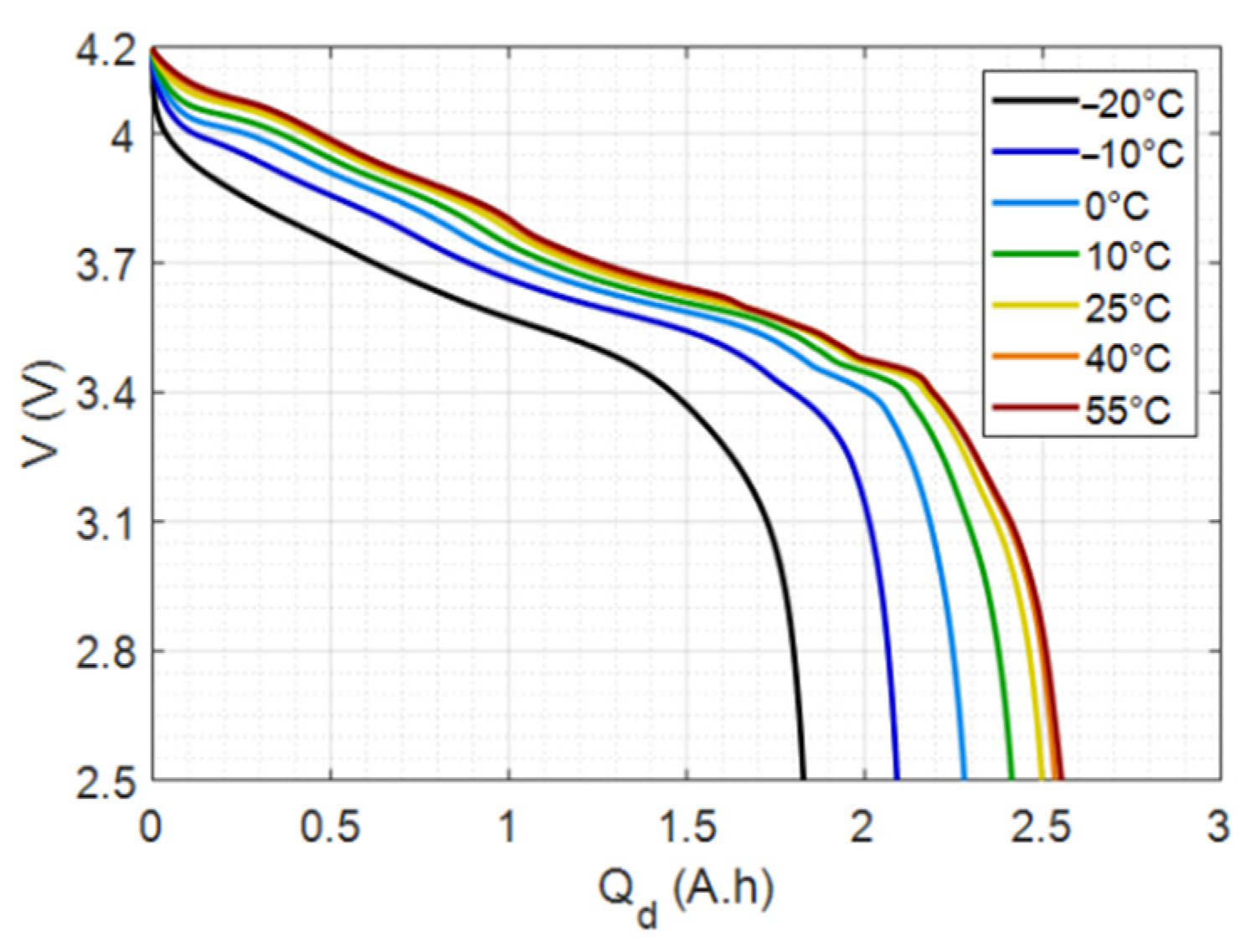
4.2. Study of the Sensitivity to Temperature

Low-current discharges at seven different temperatures were recorded over a wide range, between −20 °C and 55 °C. The C/20 discharge experimental data for each temperature are plotted in Figure 6.

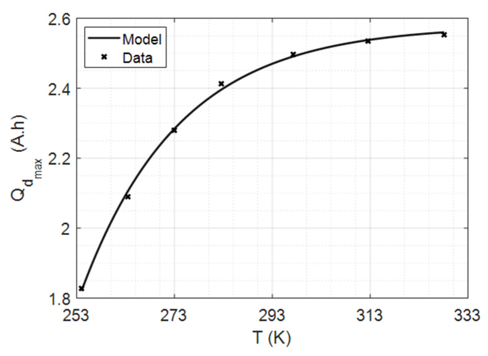
4.2.1. Maximum Capacity vs. Temperature

Two phenomena caused by temperature can be observed on those curves. Firstly, the maximum capacity $Q_{d,max}$ that can be discharged from the cell increases with temperature (Figure 6). This measured maximum capacity has been extracted and reported in Figure 7 as a function of temperature. It can be modeled empirically by using an exponential law of the Arrhenius type expressed by Equation (12). The obtained parameters are given by

Table 1. Parameters of Equation (12) model. It has a correlation coefficient R²; of 0.9984 and a maximum relative error of 0.76%.

${\mathit{Q}}_0[\mathbf{A}.\mathbf{h}]$	${\mathit{Q}}_1[\mathbf{A}.\mathbf{h}]$	${\mathit{T}}_0\left[\mathbf{K}\right]$	${\mathit{T}}_1\left[\mathbf{K}\right]$
1.82	0.76	253.99	20.09

.

$$Q_{d_{max}}\left(T\right)=Q_0+Q_1\left(1-e^{-\frac{T-T_0}{T_1}}\right)$$

(12)

This maximum capacity quantification is necessary to extend SoC definition of Equation (9) to varying temperatures with Equation (13), where $Q_d\left(V,T\right)$ is the discharged capacity of the cell at any given voltage V and temperature T.

$$SoC\left(V,T\right)=\frac{Q_{d_{max}}\left(T\right)-Q_d\left(V,T\right)}{Q_{d_{max}}\left(T\right)}.$$

(13)

Secondly, temperature also affects the smoothness of the discharge curve, with flat voltage intervals being more distinguishable at a higher temperature. This is highlighted in the IC curves in the following.

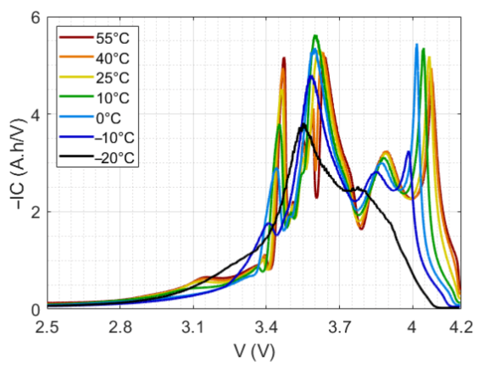
4.2.2. Incremental Capacity vs. Temperature

From the discharge curves presented in Figure 6, the IC curves have been derived and are presented in Figure 8 for all temperatures. As stated previously, the temperature affects both the maximum capacity, which is evidenced by a decreasing area under IC curves when the temperature decreases, and the smoothness of the discharge curve, which is evidenced by the number of peaks that can be distinguished. This second effect is particularly well seen in IC curves: as temperature goes down, the number of distinguishable peaks decreases. This comes from the voltage plateaus, which are less noticeable at lower temperatures, as observed previously in Figure 6.

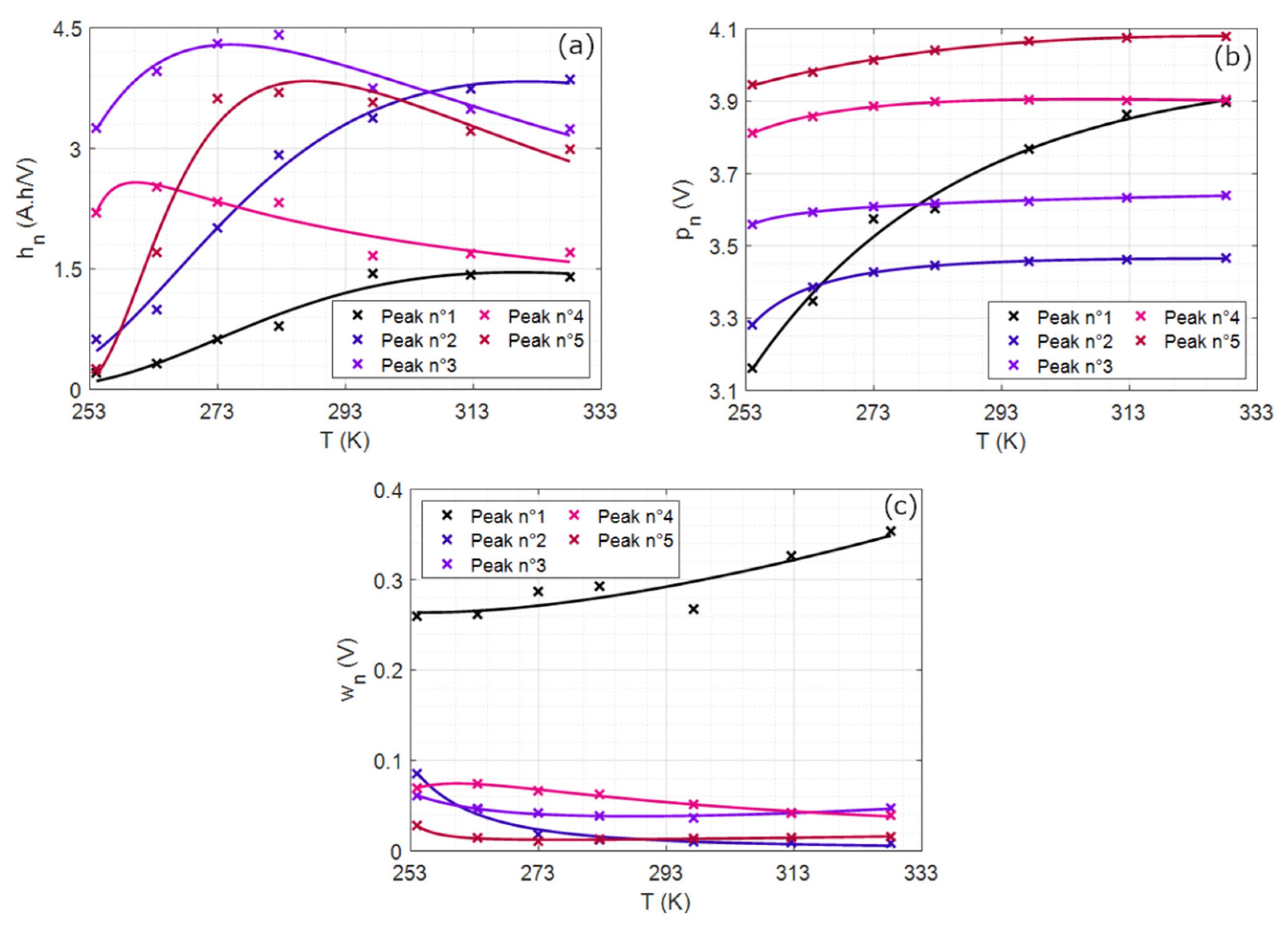
4.2.3. Peak Geometric Properties vs. Temperature and Model

The logistic model geometric parameters $h_n$, $p_n$, and $w_n$ of the five IC peaks were identified based on fitting Equation (6) to the IC curves of Figure 8 at different temperatures. The evolutions of each parameter with temperature are reported in Figure 9. As it can be seen, temperature affects each parameter of each peak in a particular way. Positions and widths have relatively monotonous evolutions with temperature: peaks tend to displace towards higher voltages while becoming thinner, except for the first peak which grows larger. This is not the case for their heights; however, where the first two peaks increase with temperature in a monotonous way, the amplitude of the three others increase from low to mid temperatures and decrease for higher temperatures.

Each peak parameter variation with temperature can be modelized using the same empirical equation, which is a modified Arrhenius law with a temperature offset expressed by

$$x_n=x_0{\left(T-T_0\right)}^{\alpha }{e}^{ \frac{E_a}{k_{B\left(T-T_0\right)}}},$$

(14)

where $x_n$ is the considered parameter (either $h_n$, $p_n$, or $w_n$), $x_0$ is a constant parameter independent of temperature, $T_0$ is the temperature offset (in K), $\alpha$ is a real power modulating the effect of the temperature pre-factor, $E_a$ is the activation energy (in J), kB is the Boltzmann constant (in J/K). Equation (14) model lines are plotted on top of identified parameters in Figure 9. It can be seen that this simple model accurately accounts for temperature variations in the geometric parameters $h_n$, $p_n$, and $w_n$.

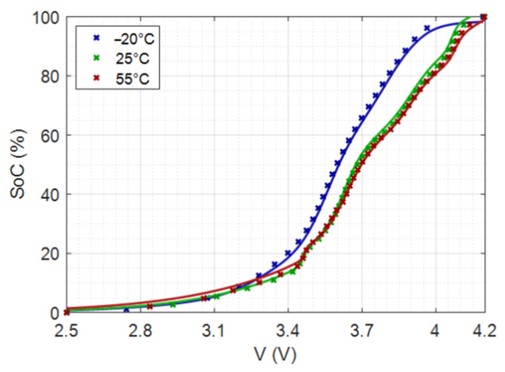
4.2.4. Application to SoC Estimation from OCV Measurements at Different Temperatures

One goal of developing such a model is to have an accurate OCV model to improve SoC estimation in BMS. For example, as the OCV depends on the temperature, having only a lookup table of the OCV measured, for example, at 25 °C, would lead to SoC estimation error if an OCV measured at a vastly different temperature is fed to the algorithm. Here, we use the bi-dimensional model of $Q=f\left(V,T\right)$ that we parameterized previously to demonstrate the usefulness of the model to take into account a wide range of thermal conditions.

Using Equations (6)–(8) and (12)–(14), a combined model of SoC as a function of voltage and temperature can be built. Figure 10 shows the comparison between the proposed model and SoC-V experimental data at three distinct temperatures. For all curves, the squared correlation coefficient R² is over 0.9997, and the maximum absolute error on the SoC is 2.22%. Hence, the complete model shows good agreement with experimental data. As can be seen in the figure, for a given measurement of voltage, absolute error for SoC estimation of up to 20% can be made over a wide temperature range if temperature is not considered in the OCV-SOC model.

This example of application demonstrates the usefulness of the model for SoC estimation considering temperature effect on the OCV. In the next paragraph, other potential interests of the model are discussed.

4.3. Other Usages of the Proposed Model

This article developed an IC model and showed a full parameterization for a lithium-ion cell. This parameterization was carried out directly with experimental data collected on a full cell and showed the performance of the model in accounting for IC peaks, OCV jumps and plateaus, as well as sensitivity of OCV to temperature. However, working with full cell data means that the contributions of the positive and negative electrode are mixed: additive for the OCV, convolutive for the IC.

Applying the same model and parameterization process to half-cell [41] data would provide additional interests for this model. Indeed, applying the model to half-cell data would yield quantitative and physical information about the chemical process happening in one electrode. Similar to the full cell, the model can describe the electrode IC curve with multiple peaks. The obtained geometric parameters $p_n$, $h_n$, and $w_n$ would then be closer to physical meaning. The position $p_n$ would directly give the potential at which a phase transition reaction happens in the electrode (in V). Moreover, the area below the IC peak can be computed from the height $h_n$ and width $w_n$. This area would give access to the amount of capacity (in Ah) exchanged in this reaction, and ultimately in the number of lithium ions. Applying the model to the positive and negative electrode half-cells would then allow us to reconstruct the full cell model as described in [30]. This would also simplify the modeling of the evolution of model parameters with temperature or SoH.

This quantitative information would also be useful for SoH monitoring. As mentioned in the introduction, ICA is an established technique in the literature and used to retrieve information about the degradation of battery electrodes. ICA can be used for a qualitative assessment of ageing and electrode degradation mechanisms [33]. When used quantitively, ICA also provides more insights into degradation [39]. Hence, the proposed logistic model would naturally couple with quantitative ICA analysis for SoH monitoring and ageing comprehension. During the ageing process, the impact of the degradation mechanisms can be synthetized in the following degradation modes: loss of lithium inventory, loss of positive and negative active matter, and ohmic resistance increase. These degradation modes impact the IC curve by shifting peaks’ positions, as well as modifying peaks’ amplitudes and widths [30]. Hence, the modification of the IC curve during the ageing process can be considered by adapting the model geometric parameters position $p_n$, height $h_n$, and width $w_n$, similar to the method carried out with the impact of temperature. We have already previously undertaken preliminary works in ICA peak tracking with ageing [29,42] and this research interest will be explored further. Additionally, the applicability of the model for incremental capacity-based SoH estimation could be investigated and compared to other proposed methods [43]. Moreover, the proposed model and its coupling with quantitative ICA analysis would naturally give tools to model the evolution of the OCV curve with ageing.

5. Conclusions

This paper developed an incremental capacity parametric model for lithium-ion batteries. It is also equivalent to a model of the OCV characteristic. The model is based on additive terms of Verhulst’s logistic equations in order to describe incremental capacity peaks geometrically. This semi-physical approach is proposed as an alternative to empirical or thermodynamic OCV models in BMS for battery state estimation and monitoring.

The model performance was compared with empirical polynomial models and was demonstrated on a commercial graphite/NCA cell. Low-current discharges performed at temperatures ranging from −20 °C to 55 °C were used to parameterize the model. The results demonstrated that the proposed model gives the advantage of:

• Offering a reversible OCV and incremental capacity model, with parameterization possible on both curves.
• Using a flexible mathematical structure, adaptable to any Li-ion electrode materials.
• Clearly describing incremental capacity peaks with model parameters giving quantitative information about each electrode chemical reactions in different battery states.
• Using a semi-physical approach requiring no prior-knowledge about electrode materials, while enabling to model the evolution of model parameters in varying battery conditions.
• Including the sensitivity of the OCV to temperature in the OCV model.

An example of practical application was proposed by using the model to estimate battery SoC from voltage and temperature measurements, improving the robustness of SoC estimation at varying temperatures in BMS. Future work includes the parameterization of the model on electrode half-cell data and the use of the model for state-of-health monitoring with incremental capacity analysis. Ultimately, the model could be used to improve the modelling of the OCV curve modifications with battery ageing.

References

1. Hoque, M.M.; Hannan, M.A.; Mohamed, A.; Ayob, A. Battery charge equalization controller in electric vehicle applications: A review. Renew. Sustain. Energy Rev. 2017, 75, 1363–1385. [Google Scholar] [CrossRef]
2. Lelie, M.; Braun, T.; Knips, M.; Nordmann, H.; Ringbeck, F.; Zappen, H.; Sauer, D.U. Battery Management System Hardware Concepts: An Overview. Appl. Sci. 2018, 8, 534. [Google Scholar] [CrossRef] [Green Version]
3. Waag, W.; Fleischer, C.; Sauer, D.U. Critical review of the methods for monitoring of lithium-ion batteries in electric and hybrid vehicles. J. Power Sources 2014, 258, 321–339. [Google Scholar] [CrossRef]
4. Meng, J.; Luo, G.; Ricco, M.; Swierczynski, M.; Stroe, D.-I.; Teodorescu, R. Overview of Lithium-Ion Battery Modeling Methods for State-of-Charge Estimation in Electrical Vehicles. Appl. Sci. 2018, 8, 659. [Google Scholar] [CrossRef] [Green Version]
5. Jossen, A. Fundamentals of battery dynamics. J. Power Sources 2006, 154, 530–538. [Google Scholar] [CrossRef]
6. Zheng, L.; Zhang, L.; Zhu, J.; Wang, G.; Jiang, J. Co-estimation of state-of-charge, capacity and resistance for lithium-ion batteries based on a high-fidelity electrochemical model. Appl. Energy 2016, 180, 424–434. [Google Scholar] [CrossRef]
7. Zhang, C.; Wang, L.Y.; Li, X.; Chen, W.; Yin, G.G.; Jiang, J. Robust and Adaptive Estimation of State of Charge for Lithium-Ion Batteries. IEEE Trans. Ind. Electron. 2015, 62, 4948–4957. [Google Scholar] [CrossRef]
8. Kang, L.; Zhao, X.; Ma, J. A new neural network model for the state-of-charge estimation in the battery degradation process. Appl. Energy 2014, 121, 20–27. [Google Scholar] [CrossRef]
9. Geng, Z.; Wang, S.; Lacey, M.J.; Brandell, D.; Thiringer, T. Bridging physics-based and equivalent circuit models for lithium-ion batteries. Electrochim. Acta 2021, 372, 137829. [Google Scholar] [CrossRef]
10. Li, W.; Zhang, J.; Ringbeck, F.; Jöst, D.; Zhang, L.; Wei, Z.; Sauer, D.U. Physics-informed neural networks for electrode-level state estimation in lithium-ion batteries. J. Power Sources 2021, 506, 230034. [Google Scholar] [CrossRef]
11. Pei, L.; Wang, T.; Lu, R.; Zhu, C. Development of a voltage relaxation model for rapid open-circuit voltage prediction in lithium-ion batteries. J. Power Sources 2014, 253, 412–418. [Google Scholar] [CrossRef]
12. Dubarry, M.; Svoboda, V.; Hwu, R.; Liaw, B.Y. Capacity loss in rechargeable lithium cells during cycle life testing: The importance of determining state-of-charge. J. Power Sources 2007, 174, 1121–1125. [Google Scholar] [CrossRef]
13. Nitta, N.; Wu, F.; Lee, J.T.; Yushin, G. Li-ion battery materials: Present and future. Mater. Today 2015, 18, 252–264. [Google Scholar] [CrossRef]
14. Farmann, A.; Sauer, D.U. A study on the dependency of the open-circuit voltage on temperature and actual aging state of lithium-ion batteries. J. Power Sources 2017, 347, 1–13. [Google Scholar] [CrossRef]
15. Lin, X.; Perez, H.E.; Mohan, S.; Siegel, J.; Stefanopoulou, A.G.; Ding, Y.; Castanier, M.P. A lumped-parameter electro-thermal model for cylindrical batteries. J. Power Sources 2014, 257, 1–11. [Google Scholar] [CrossRef]
16. Zhang, Y.C.; Briat, O.; Boulon, L.; Deletage, J.-Y.; Martin, C.; Coccetti, F.; Vinassa, J.-M. Non-isothermal Ragone plots of Li-ion cells from datasheet and galvanostatic discharge tests. Appl. Energy 2019, 247, 703–715. [Google Scholar] [CrossRef]
17. Zhang, R.; Xia, B.; Li, B.; Cao, L.; Lai, Y.; Zheng, W.; Wang, H.; Wang, W.; Wang, M. A Study on the Open Circuit Voltage and State of Charge Characterization of High Capacity Lithium-Ion Battery Under Different Temperature. Energies 2018, 11, 2408. [Google Scholar] [CrossRef] [Green Version]
18. Zhang, C.; Jiang, J.; Zhang, L.; Liu, S.; Wang, L.; Loh, P.C. A Generalized SOC-OCV Model for Lithium-Ion Batteries and the SOC Estimation for LNMCO Battery. Energies 2016, 9, 900. [Google Scholar] [CrossRef] [Green Version]
19. Weng, C.; Sun, J.; Peng, H. A unified open-circuit-voltage model of lithium-ion batteries for state-of-charge estimation and state-of-health monitoring. J. Power Sources 2014, 258, 228–237. [Google Scholar] [CrossRef]
20. Ohzuku, T.; Ueda, A. Phenomenological Expression of Solid-State Redox Potentials of LiCoO2, LiCo1/2Ni1/2O2, and LiNiO2 Insertion Electrodes. J. Electrochem. Soc. 1997, 144, 2780. [Google Scholar] [CrossRef]
21. Ali, S.A.H. Thermodynamic analysis of lithium ion cells. Ionics 2005, 11, 410–413. [Google Scholar] [CrossRef]
22. Karthikeyan, D.K.; Sikha, G.; White, R.E. Thermodynamic model development for lithium intercalation electrodes. J. Power Sources 2008, 185, 1398–1407. [Google Scholar] [CrossRef]
23. Lavigne, L.; Sabatier, J.; Francisco, J.M.; Guillemard, F.; Noury, A. Lithium-ion Open Circuit Voltage (OCV) curve modelling and its ageing adjustment. J. Power Sources 2016, 324, 694–703. [Google Scholar] [CrossRef]
24. Birkl, C.R.; McTurk, E.; Roberts, M.R.; Bruce, P.G.; Howey, D. A Parametric Open Circuit Voltage Model for Lithium Ion Batteries. J. Electrochem. Soc. 2015, 162, A2271–A2280. [Google Scholar] [CrossRef] [Green Version]
25. Li, X.; Jiang, J.; Wang, L.Y.; Chen, D.; Zhang, Y.; Zhang, C. A capacity model based on charging process for state of health estimation of lithium ion batteries. Appl. Energy 2016, 177, 537–543. [Google Scholar] [CrossRef]
26. Weng, C.; Feng, X.; Sun, J.; Peng, H. State-of-health monitoring of lithium-ion battery modules and packs via incremental capacity peak tracking. Appl. Energy 2016, 180, 360–368. [Google Scholar] [CrossRef] [Green Version]
27. Zheng, L.; Zhu, J.; Lu, D.D.-C.; Wang, G.; He, T. Incremental capacity analysis and differential voltage analysis based state of charge and capacity estimation for lithium-ion batteries. Energy 2018, 150, 759–769. [Google Scholar] [CrossRef]
28. Bian, X.; Liu, L.; Yan, J. A model for state-of-health estimation of lithium ion batteries based on charging profiles. Energy 2019, 177, 57–65. [Google Scholar] [CrossRef]
29. Maures, M.; Zhang, Y.; Martin, C.; Delétage, J.-Y.; Vinassa, J.-M.; Briat, O. Impact of temperature on calendar ageing of Lithium-ion battery using incremental capacity analysis. Microelectron. Reliab. 2019, 100–101, 113364. [Google Scholar] [CrossRef]
30. Dubarry, M.; Truchot, C.; Liaw, B.Y. Synthesize battery degradation modes via a diagnostic and prognostic model. J. Power Sources 2012, 219, 204–216. [Google Scholar] [CrossRef]
31. Baure, G.; Dubarry, M. Synthetic vs. Real Driving Cycles: A Comparison of Electric Vehicle Battery Degradation. Batteries 2019, 5, 42. [Google Scholar] [CrossRef] [Green Version]
32. Riviere, E.; Sari, A.; Venet, P.; Meniere, F.; Bultel, Y. Innovative Incremental Capacity Analysis Implementation for C/LiFePO4 Cell State-of-Health Estimation in Electrical Vehicles. Batteries 2019, 5, 37. [Google Scholar] [CrossRef] [Green Version]
33. Mathieu, R.; Briat, O.; Gyan, P.; Vinassa, J.-M. Comparison of the impact of fast charging on the cycle life of three lithium-ion cells under several parameters of charge protocol and temperatures. Appl. Energy 2020, 283, 116344. [Google Scholar] [CrossRef]
34. Krupp, A.; Ferg, E.; Schuldt, F.; Derendorf, K.; Agert, C. Incremental Capacity Analysis as a State of Health Estimation Method for Lithium-Ion Battery Modules with Series-Connected Cells. Batteries 2020, 7, 2. [Google Scholar] [CrossRef]
35. Verhulst, P.-F. Recherches mathématiques sur la loi d’accroissement de la population. Nouv. Mém. L’académie Des Sci. B-Lett. Brux. Tome XVIII 1845, 18, 1–38. [Google Scholar]
36. Liu, C.; Neale, Z.G.; Cao, G. Understanding electrochemical potentials of cathode materials in rechargeable batteries. Mater. Today 2016, 19, 109–123. [Google Scholar] [CrossRef]
37. Yang, S.; Zhang, C.; Jiang, J.; Zhang, W.; Gao, Y.; Zhang, L. A voltage reconstruction model based on partial charging curve for state-of-health estimation of lithium-ion batteries. J. Energy Storage 2021, 35, 102271. [Google Scholar] [CrossRef]
38. Schindler, S.; Baure, G.; Danzer, M.A.; Dubarry, M. Kinetics accommodation in Li-ion mechanistic modeling. J. Power Sources 2019, 440, 227117. [Google Scholar] [CrossRef]
39. Fly, A.; Chen, R. Rate dependency of incremental capacity analysis (dQ/dV) as a diagnostic tool for lithium-ion batteries. J. Energy Storage 2020, 29, 101329. [Google Scholar] [CrossRef]
40. Dreyer, W.; Jamnik, J.; Guhlke, C.; Huth, R.; Moškon, J.; Gaberšček, M. The thermodynamic origin of hysteresis in insertion batteries. Nat. Mater. 2010, 9, 448–453. [Google Scholar] [CrossRef]
41. Waldmann, T.; Iturrondobeitia, A.; Kasper, M.; Ghanbari, N.; Aguesse, F.; Bekaert, E.; Daniel, L.; Genies, S.; Gordon, I.J.; Löble, M.W.; et al. Review—Post-Mortem Analysis of Aged Lithium-Ion Batteries: Disassembly Methodology and Physico-Chemical Analysis Techniques. J. Electrochem. Soc. 2016, 163, A2149–A2164. [Google Scholar] [CrossRef]
42. Maures, M.; Capitaine, A.; Delétage, J.-Y.; Vinassa, J.-M.; Briat, O. Lithium-ion battery SoH estimation based on incremental capacity peak tracking at several current levels for online application. Microelectron. Reliab. 2020, 114, 113798. [Google Scholar] [CrossRef]
43. Jiang, B.; Dai, H.; Wei, X. Incremental capacity analysis based adaptive capacity estimation for lithium-ion battery considering charging condition. Appl. Energy 2020, 269, 115074. [Google Scholar] [CrossRef]
Figure 1. (a) Low-current discharge measured at 25 °C and C/20, and (b) corresponding incremental capacity curve (Note: during the discharge, IC peaks are negative, but are plotted positively here for clarity).
Batteries 08 00039 g001
Figure 2. Example of a logistic function Equation (2) (blue) and its derivative Equation (3) (red) with parameters: y 0 = 2 , K = 3000 and r = 14 . Geometric peak parameters position p , height h , and width w from Equation (5) are illustrated.
Batteries 08 00039 g002
Figure 3. Accuracy comparison between polynomial models (n°1 and 2) and the proposed model (n°3) for a given number of parameters N : Coefficient of determination R 2 and RMSE ϵ of the models against (left, (a,c)) capacity vs. voltage data, and (right, (b,d)) incremental capacity vs. voltage data.
Batteries 08 00039 g003
Figure 4. Reconstruction of the proposed logistic model against experimental data at 25 °C on (a) the voltage curve and (b) the IC curve. Grey curves correspond to additive terms of Equation (5), adding up to the reconstructed model in green.
Batteries 08 00039 g004
Figure 5. Comparison between polynomial models (n°1 and 2) and the proposed model (n°3) against experimental data at 25 °C (a) on the discharge curve and (b) corresponding IC curve.
Batteries 08 00039 g005
Figure 6. Low-current discharge curves measured at different temperatures.
Batteries 08 00039 g006
Figure 7. Maximum discharged capacity measured against test temperature and Equation (12) model.
Batteries 08 00039 g007
Figure 8. Incremental capacity curves at different temperatures.
Batteries 08 00039 g008
Figure 9. Geometric parameters of incremental capacity peaks against temperature: (a) heights h n , (b) positions p n , and (c) widths w n . Each cross corresponds to the value found for each temperature using Equation (6) model, while each line is a temperature model of each parameter using Equation (14).
Batteries 08 00039 g009
Figure 10. Estimation of the SoC at different voltages and temperatures using the proposed S o C = f ( V , T ) model. Crosses represent experimental data while lines are the combined models.
Batteries 08 00039 g010