Comparison of Capacity Fade for the Constant Current and WLTC Drive Cycle Discharge Modes for Commercial LiFeYPO₄ Cells Used in xEV Vehicles

Abstract

In this paper, capacity fade of LiFeYPO₄/graphite commercial cells during 116 cycles under different temperatures is studied. The cells were discharged in two modes, during Drive Cycle (DrC) discharge cycles the cell was discharged with current waveform calculated for example battery electric vehicle (BEV) under WLTC 3b drive cycle conditions, whereas during Constant Current (CC) discharge cycles the cell was discharged with a constant current of the same root mean square of the current, as the WLTC 3b current waveform and with the same depth of discharge. All the cells were charged in constant current/constant voltage mode. Two fresh cells were used for each discharge mode at 25 °C and as the results were similar, only one cell per discharge mode was used at the other temperatures 5 °C and 45 °C. Furthermore, simulation P2D model of calendar and cycle life was calibrated based on experimental data. SoC floating was observed during cycling for both discharge modes, accompanied with slight increase in end discharge voltage and growth of energy efficiency. Concluding the results for 25 °C, not waveform character, but the amount of electric charge in combination with calendar aging has the most effect on the cycle life, which is also proved by the simulation. For 5 °C, the capacity fade is milder for DrC discharge cycles, but simulation results do not prove that, which would demand further investigation. The results for 45 °C are apparently dependent on a higher amount of discharged and charged electric charge and influenced by calendar life, simulated capacity fade corresponds quite well to the experiment. The best State of Health (SoH) simulation results are for temperature 45 °C, RMSE is 0.10% SoH, for the other temperatures RMSE is 0.20 and 0.93% SoH for 25 and 5 °C, respectively.

1. Introduction

1.1. xEV

Battery electric vehicles (BEV), plug-in hybrid electric vehicles (PHEV), hybrid electric vehicles (HEV) and fuel cell electric vehicles (FCEV), together referred to as xEV, are of growing importance in road transportation recently.

Critical part of xEV in terms of performance and usability is a traction battery, which not only limits reachable range of the vehicle, but also influences vehicle life cycle economics due to calendar and cycle aging of electrochemical cells. Both calendar and cycle aging are complex processes depending on many circumstances, such as chemistry of anode and cathode or storage and operational conditions of the battery [1]. Calendar and cycle aging are often considered as additive, but interactions may occur. Both mechanisms lead to capacity fade, which can be measured as the gradual decrease in state of health (SoH), which is the ratio between actual and fresh cell capacity under the same conditions, such as fully charged cell, discharging current, temperature, or cut-off voltage.

1.2. LiFeYPO₄

LiFePO₄ and LiFeYPO₄ cathodes are widely used in the automotive and bus industries. When LiFePO₄ cathode is doped by yttrium, it has a remarkable effect on battery performance, such as charge/discharge and capacity-voltage curves [2]. Furthermore, there is a difference is in the behavior of chemical elements yttrium and iron. While iron is very susceptible to oxidation and reactions with other chemical compounds, the element yttrium is more chemically stable. The result is much stronger chemical stability and durability, especially in terms of calendar life [3].

1.3. Testing of Cycle Aging

LiFe(Y)PO₄/graphite commercial batteries are tested by manufacturers. The manufacturers or suppliers are providing data about cycle aging under specific operational conditions, which may be sufficiently specified [4] or at least partly specified [5]. Researchers have performed many experimental tests focused on cycle aging, including the influence of varying current rates and DoDs (Depth of Discharges) [6]; operating conditions typical to high-power automotive applications, such as high charge and discharge rate; elevated temperatures and wide state-of-charge windows [7]; or influence of different test temperatures from −10 up to 45 °C [8]. All the above mentioned and other published experiments were performed with Constant Current (CC) discharging and Constant Current/Constant Voltage (CC/CV) charging. The character of charging is the same for testing batteries in laboratory conditions and in real operation of traction battery, whereas the character of discharging is of a significant difference. When tested under typical laboratory conditions, batteries are discharged in CC mode, while when used in xEV, there is a strong time dependency of instantaneous values of traction current. The traction current profile is rather similar to the character of drive cycles, such as Worldwide harmonized Light vehicles Test Cycle (WLTC), New European Driving Cycle (NEDC), etc. There are experimental results on testing traction batteries during real driving [9], as well as comparison of battery degradation for synthetic vs. real driving cycles [10], but to the best of the authors’ knowledge, no comparison of cycle aging under CC/CV vs. drive cycle conditions have been published yet.

1.4. Simulation of Cycle Aging

Battery degradation models fall into model-based estimation methods, that can be used for estimation of battery internal states, such as SoH [11]. Model-based aging studies mainly include empirical model [12], semi-empirical and electrochemical models [13,14]. Owing to the fact that the aforementioned SoH cannot be measured directly, more accurate degradation models for reliable SoH estimations are of critical importance. It is obvious that a substantial part of a performance of the BMSs relies on that models.

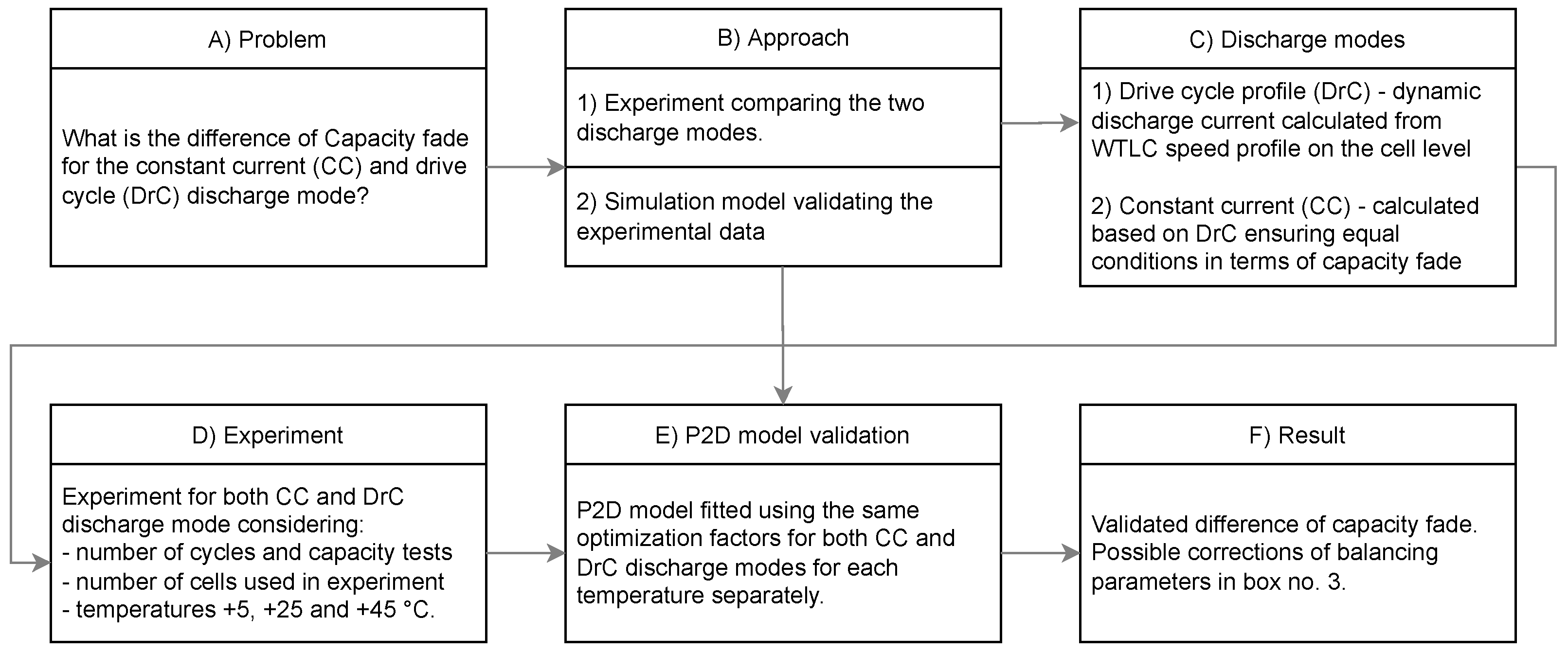
1.5. Objectives of This Paper

This paper aims to answer two basic questions that have not yet been answered anywhere:

(a)

What is the difference of capacity fade for the CC and DrC discharge mode?

(b)

How can be commonly available CC discharging results of capacity fade understood in terms of supposed dynamic WLTC discharging profile representing real performance of the xEV battery?

This paper aims to present a comparison between cycle aging performed under two different characters of discharging and charging:

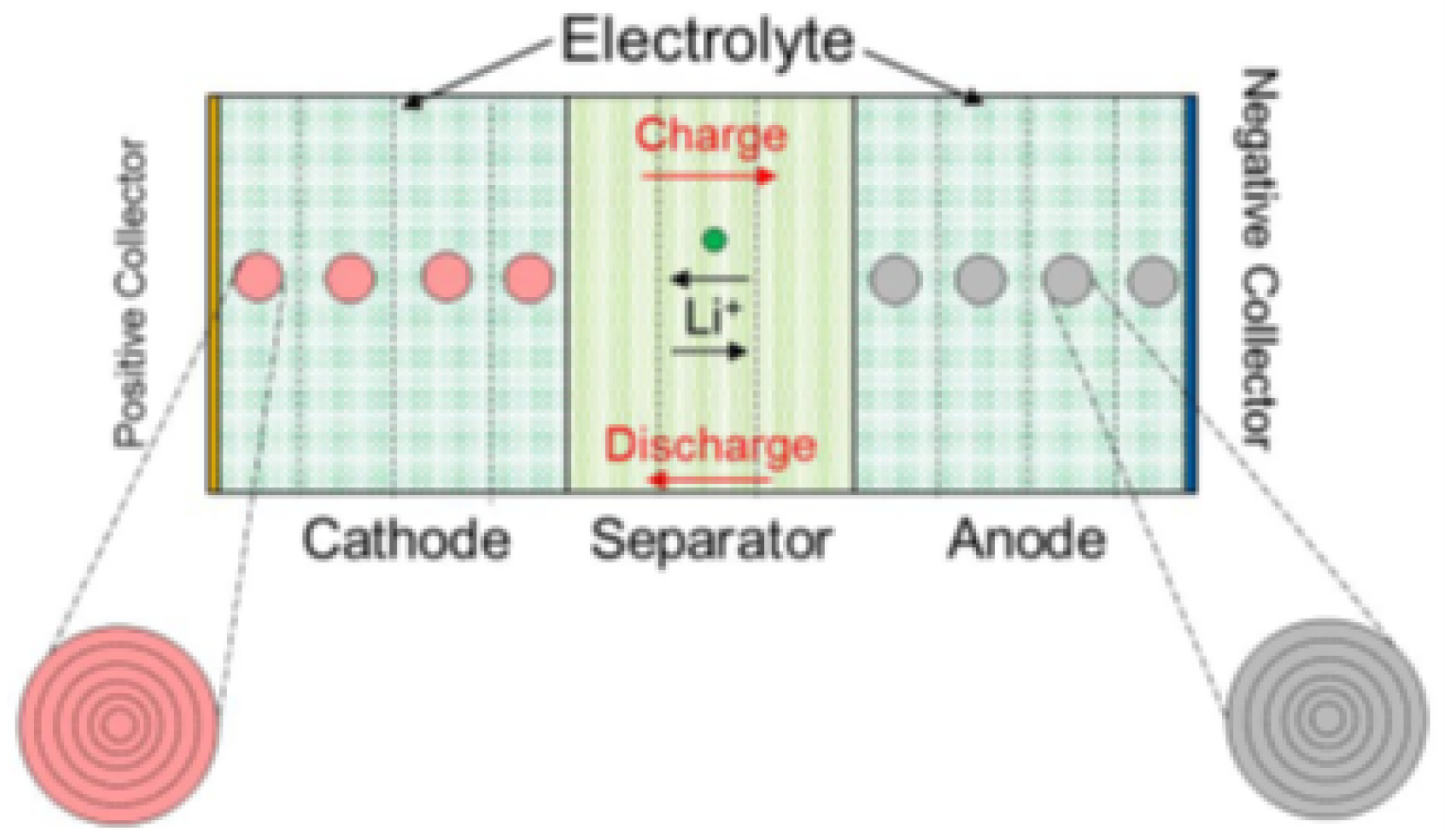
• CC discharge cycles: this is the usual test mode, when the battery is discharged in CC mode and charged in CC/CV mode.
• Drive cycle discharge cycles: battery is discharged with a current waveform based on drive cycle and it is charged in CC/CV mode.

Furthermore, it aims to find relation between parameters of cyclic testing of CC discharge cycles and drive cycle discharge cycles with the same effect on capacity fade. All the work is focused on automotive applications.

2. Methods of Comparison

The method used for studying the difference of Capacity fade for the two discharge modes is summarized in Figure 1. Each box in the figure is referenced to appropriate section of this paper.

2.1. General Considerations

As this work is focused on automotive applications, three different temperatures, namely, 5, 25 and 45 °C are studied. The scope of temperatures does not include temperatures below 0 °C, as 1. negative temperatures significantly worsen capacity fade for the selected battery chemistry, 2. traction battery of xEV is anticipated to operate mostly within temperatures above 0 °C. Due to limited time available, 100 cycles are carried out under different cycle conditions for each commercial cell tested, whereas capacity tests occur every 25 cycles. Altogether with formatting and capacity tests, 116 cycles were measured for each cell. Readers are referred to [15] for cycle life behavior of LFP cells in the range of thousands of cycles.

Experimental results serve as data for calibrating the capacity fade of an electrochemical pseudo 2-D (P2D) model.

The approach described in this Section 2 can be understood as a proposal of conversion between cycle life with discharging in CC and DrC discharge modes.

2.2. Battery Chemistry Selection

For the experiment, the LiFeYPO₄ Winston 40 Ah battery was selected for several reasons. Lithium iron phosphate (LFP) and lithium iron yttrium phosphate (LYP) battery is a proven and widely used technology in applications where a lower energy density was accepted. However, in the last year, we see more often its utilization in personal cars for its lower price, safety, lifetime, and improved energy density [16,17,18].

Further, the LYP battery was selected due to its availability on the market and the need to purchase a certain quantity for the experiment. LiFeYPO₄ Winston 40 Ah battery model was used based on previous experience of the research team and already existing mathematical model validated during previous research [19].

2.3. Electric Current Waveform for the Experiment

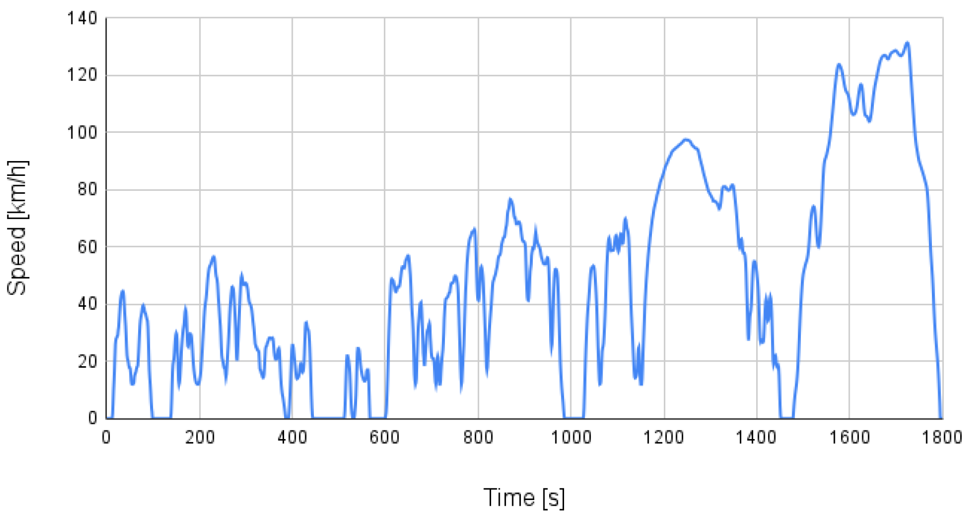
2.3.1. Vehicle Test Cycle

The Worldwide harmonized Light vehicles Test Cycles (WLTC) are chassis dynamometer tests for the determination of emissions and fuel consumption from light-duty vehicles. These cycles are part of the Worldwide harmonized Light vehicles Test Procedures (WLTP), which completely replaced the former European NEDC procedure in 2019. The WLTC is a cycle consisting of four dynamic phases (52% urban and 48% non-urban) representing real driving [20].

To reproduce real-world vehicle behavior and to generate authentic drive cycle discharge cycles current waveform, the WLTC Class 3b depicted in Figure 2 was used as a reference for the purpose of this paper, as it corresponds to cars driven in Europe.

2.3.2. Battery Electric Vehicle Model

A vehicle dynamic model of a personal battery electric vehicle (BEV) was needed to extract the electric current waveform, consequently used for the experiment as a cell current. A GT-SUITE example model of the BEV by Gamma Technologies was used as a basis [21].

The mathematical model of the longitudinal vehicle dynamic model was used to translate the vehicle speed curve into the electric current. This simplified model assumes that the vehicle performs only forward movement and considers all energy-requiring aspects, mainly aerodynamic drag, rolling resistance, gradient force, inertial force, and then powertrain losses in the gearbox, electric motor, and battery itself. Auxiliary consumption for on-board systems was set as a constant value. The vehicle model from GT-Suite performed forward dynamic analysis thanks to the driver model that follows the required speed curve and controls the throttle. The final electric current was acquired by translating the power requirement from the driver according to the battery conditions (temperature, SOC, voltage) using the GT-AutoLion battery model.

This model was then adjusted for the purpose of the experiment. The original sub-model of the battery was replaced with the LiFeYPO₄ Winston model using the pre-calibrated GT-AutoLion block. Several vehicle parameters were changed to the characteristics of an urban middle-sized BEV, where LFP and LYP battery technologies are utilized and have further potential.

The final designed traction battery consists of 164 cells, where 82 cells are connected in series with two parallel branches. The battery weighs 270 kg and has a nominal voltage of 277 V and the total energy of 22.18 kWh. The curb weight of the vehicle was set to 1300 kg.

Aerodynamic coefficient and front area were increased compared to the original GT-SUITE example model since urban vehicles are more angulated.

Table 1. Modified vehicle parameters and parameters that influence the performance simulation the most.

Component	Variable	Value	Unit
Vehicle	Mass	1300	kg
Vehicle	Front area	2.1	m${}^2$
Vehicle	Drag coefficient	0.31	-
Tire	Rolling resistance coefficient	0.015	-
Differential	Final Drive Ratio	7.05	-
Differential	Efficiency	0.95	-
Electric motor	Efficiency	original map fcn (rpm. Nm)	-
Battery cell	Capacity	40	Ah
Battery cell	Nominal voltage	3.3	V
Battery cell	Weight	1600	g
Battery system	Connection	82 ser × 2 par	-
Battery system	Nominal voltage	277.2	V
Battery system	Total energy	22.18	kWh
Boundary condition	Auxiliary power	300	W
Boundary condition	Passenger and Cargo Mass	80	kg
Boundary condition	The initial State of Charge	100	%

shows modified vehicle parameters and parameters that influence the performance simulation the most. If the parameter is not mentioned in the table, it was not changed compared to the original GT-SUITE example model.

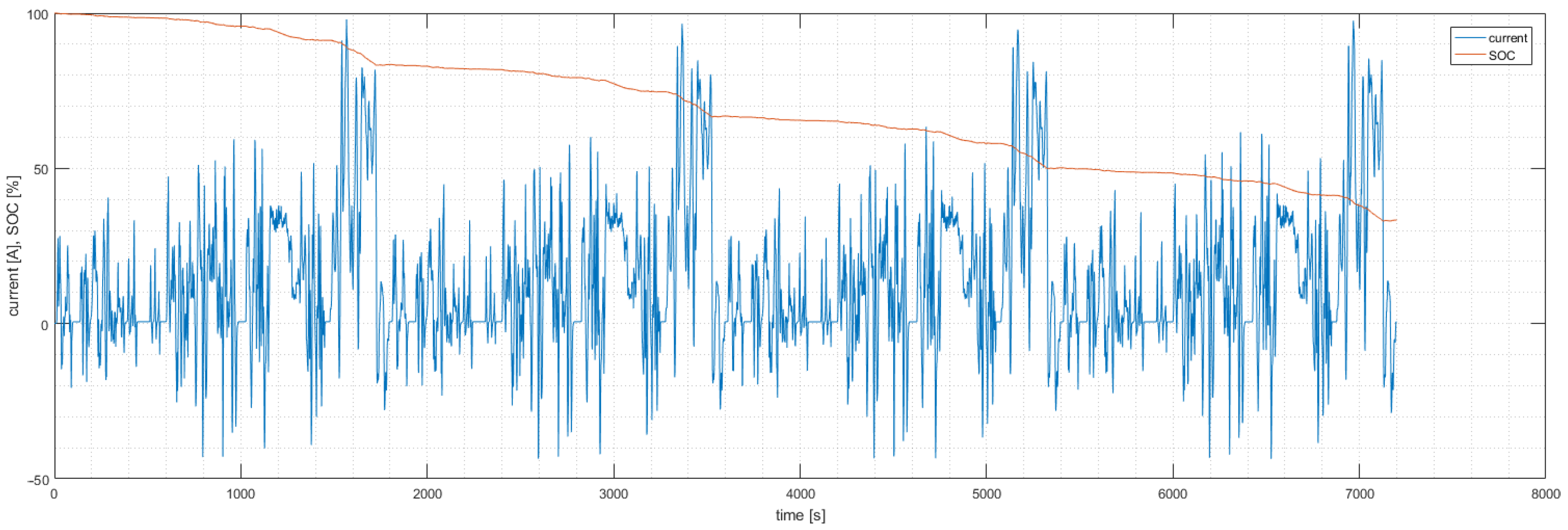
2.4. Drive Cycle Mode

The WLTC 3b drive cycle was performed four times consecutively with the above-described battery-electric vehicle model to create a representative electric current waveform of a traction battery in real conditions. The vehicle model fulfills the required velocity profile and no battery derating occurs.

Figure 3 below shows the resulting electric current of the BEV model. The initial state of charge (SoC) is 100% and at the end of the simulation, the value of SoC is 33.33%, which corresponds to 66.67% DoD.

The final drive cycle discharge cycle for the experiment consists of the presented electric current followed by CC/CV charging.

2.5. Continuous Current Mode

One of the research goals of this paper is to create a CC profile that would represent the dynamic load of the electric current and have the same effect on the capacity fade as the drive cycle dynamic profile.

According to various sources [1,22,23], capacity fade is mostly enhanced by high temperatures, high cycling rate, and high DoD of the battery cell. Therefore, the RMS of the electric current from the drive cycle modes is used as a reference and the main impact variable which causes the capacity fade taking into account the heating effect of the electric current.

The RMS of the electric current under the drive cycle mode of the vehicle model described in Section 2.4 above equals 26 Amperes per cell or a C-rate of 0.65 C. This constant current value therefore corresponds to the current of the drive cycle mode vehicle model and is then used as the set CC discharge current for the experiment.

2.6. Simulation

In this paper, the pseudo-two dimensional model (the P2D) within the cell simulation tool GT-AutoLion (version 2022) was used for capacity fade model calibration through the selected aging mechanisms. The GT-AutoLion calendar aging model was calibrated based on experimental results for a 25 °C calendar aging sample cell (referred to as CalAge). Parameters of the cycle aging model were then calibrated separately for each temperature based on experimental results of all the remaining cells.

3. Experiment Set-Up

The experimental set-up is apparent in Figure 4. Both the supply and load are programmable devices connected in parallel to the battery. The diode is used for protection of the power supply. Significant quantities are measured using a DAQ card installed in the Control PC and using embedded means of individual devices.

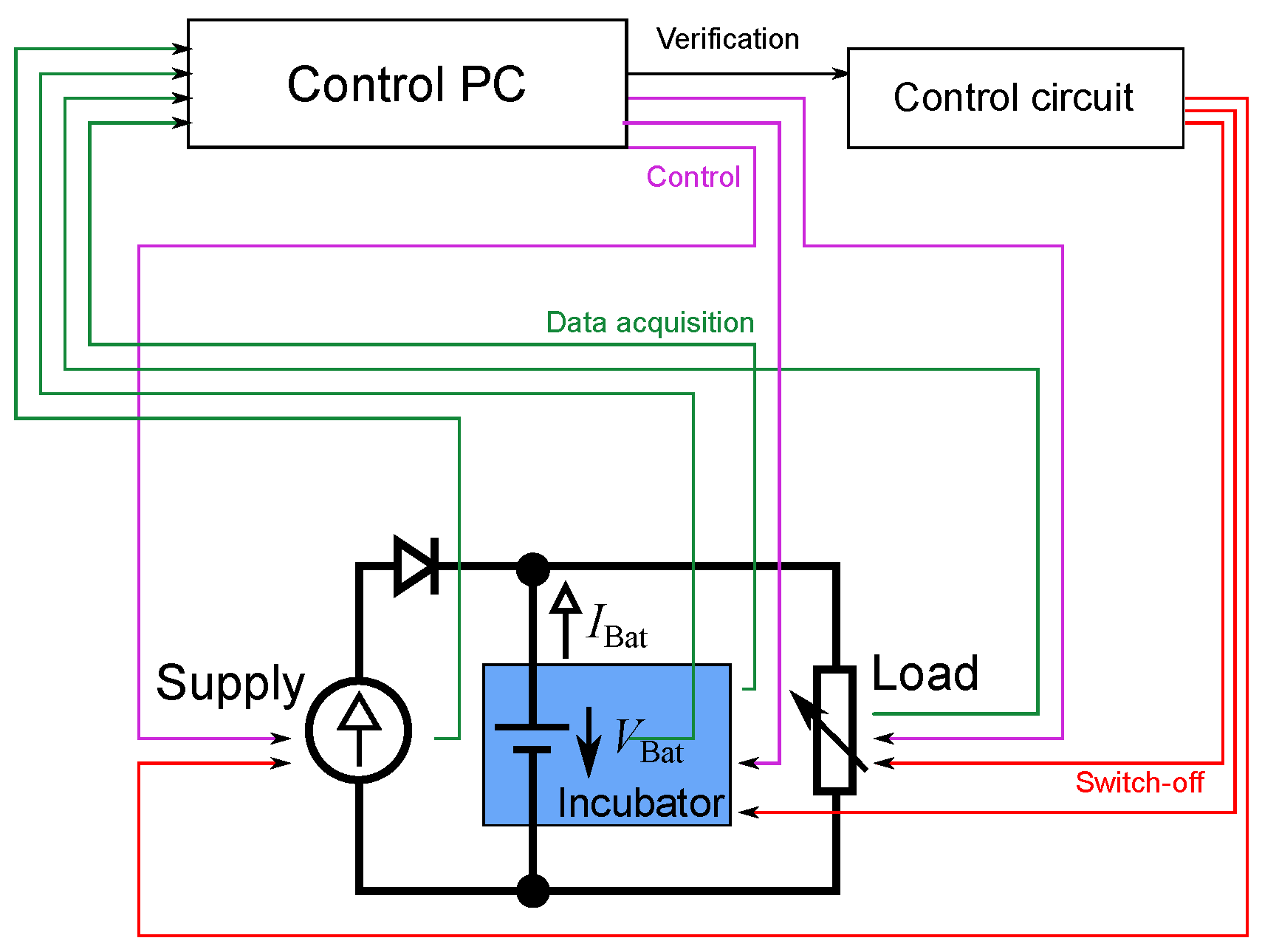
3.1. Equipment

An A6kW was used as a power supply. A protective diode in an external circuit caused a reverse current of 16 $\mathsf{\mu }$A in the case of switched off output of the power supply. As the current sensor was connected at the common branch of the circuit, this current was considered properly.

An EL9080-400 was used as a programmable power load. An analog interface was used to build the drive-cycle waveform in combination with the maximum charging current offset compensation using power supply A6kW.

A NI PCIe-6341 DAQ card as a part of the control PC was used for data acquisition through the terminal block SCB-68A. The battery voltage was measured directly by the DAQ card, the battery current was measured by the sensor Telcon HT300M and the temperatures were measured by LM19 sensors. The signals of current and temperatures were applied to the analog inputs of the DAQ card.

The software for experiment process control was developed in LabVIEW environment by the authors.

3.2. Cycling Specification

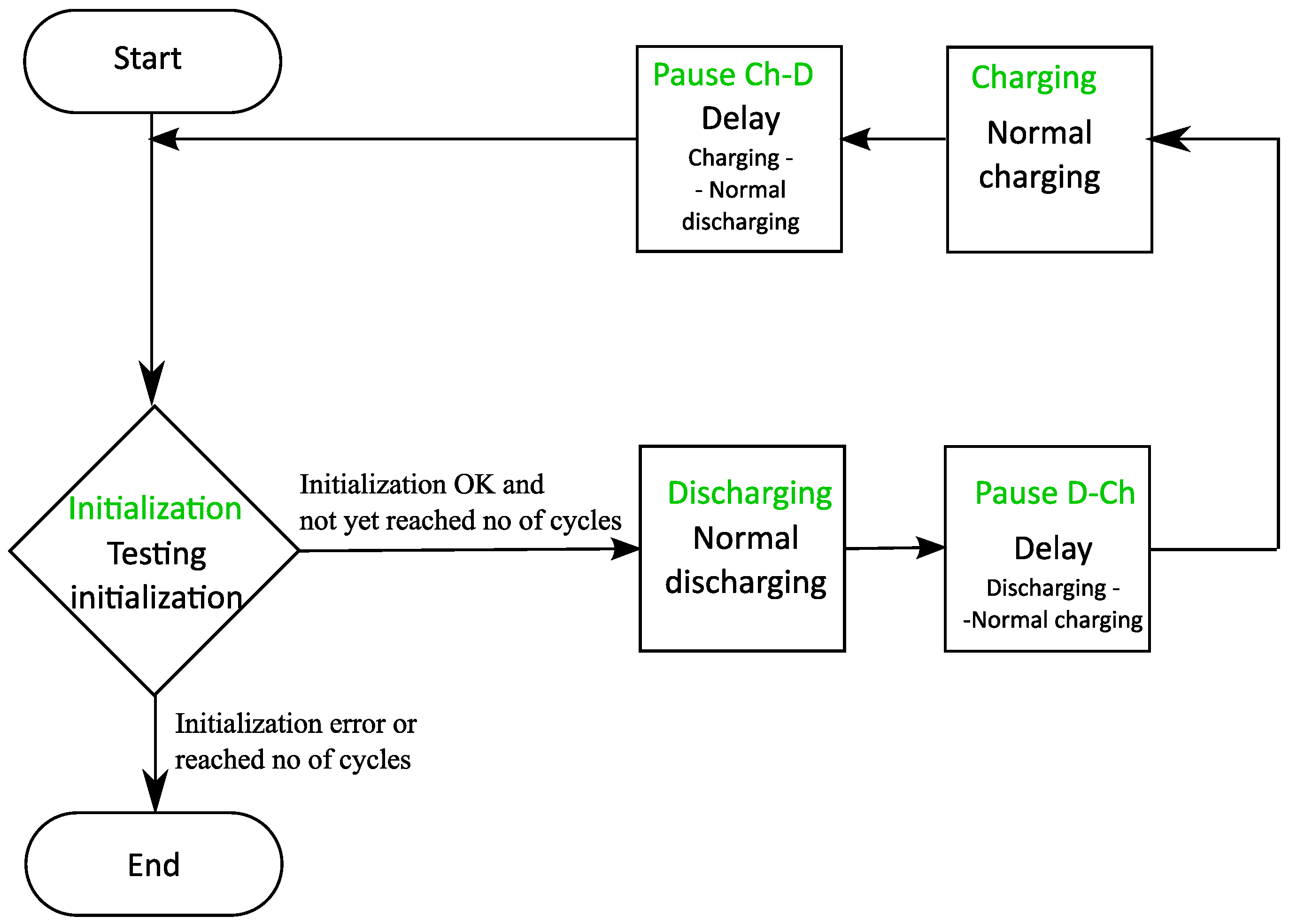
3.2.1. State Machine

The state machine depicted in Figure 5 represents the cycle aging experimental control process.

One normal cycle is composed of one consecutive discharging and charging. Discharging can be carried out either in CC or DrC mode, charging always occurs in CC/CV mode.

Initial 0.5 C charging followed by five cycles of 50% DoD and 0.5 C discharging and charging currents are always used for initiation, as it is recommended by the supplier [24], because the capacity may increase in early stages of life [6].

A certain number of normal cycles followed by two capacity tests is hereinafter referred to as a metacycle. The reason for two capacity tests is an increased repeatability due to the sensitivity of measured capacity on the conditions of the cycle preceding the capacity test cycle. Several consecutive metacycles are used for the cycle aging experiment.

3.2.2. Parameters

Common static parameters throughout all the cycles based on the supplier specification of the commercial cell [25] and LFP/LYP cells testing experience are listed below:

• CC mode Charging current $0.5\mathrm{C}$;
• charging voltage $3.7\mathrm{V}$;
• CV mode Charging cut-off current $0.025\mathrm{C}$;
• delay between discharging and charging $1800\mathrm{s}$;
• delay between charging and discharging $1800\mathrm{s}$.

Table 2. Variable parameters of cyclic tests performed in CC discharging mode. Charging is always in CC/CV mode.

Indication	$\mathit{NumCycles}$	$\mathit{EndCycleNum}$	${\mathit{I}}_{\mathit{Dis}}$	${\mathit{V}}_{\mathit{Dis}}$	${\mathit{T}}_{\mathit{Dis}}$	${\mathit{T}}_{\mathit{Ch}}$	$\mathit{DoD}$
—	$\left(1\right)$	$\left(1\right)$	$\left(\mathrm{xC}\right)$	$\left(\mathrm{V}\right)$	$(°\mathrm{C})$	$(°\mathrm{C})$	$(\%)$
0.5 C charge	1	1	0	2.8	25	25	0
formatting	5	6	0.5	2.8	25	25	50
capacity test	2	8	0.5	2.8	25	25	max
25 normal cycles	25	33	0.65	2.4	$\left\{T_{Dis}\right\}$	$\left\{T_{Ch}\right\}$	66.67
capacity test	2	35	0.5	2.8	25	25	max
25 normal cycles	25	60	0.65	2.4	$\left\{T_{Dis}\right\}$	$\left\{T_{Ch}\right\}$	66.67
capacity test	2	62	0.5	2.8	25	25	max
25 normal cycles	25	87	0.65	2.4	$\left\{T_{Dis}\right\}$	$\left\{T_{Ch}\right\}$	66.67
capacity test	2	89	0.5	2.8	25	25	max
25 normal cycles	25	114	0.65	2.4	$\left\{T_{Dis}\right\}$	$\left\{T_{Ch}\right\}$	66.67
capacity test	2	116	0.5	2.8	25	25	max

shows the cycle configuration for one particular test cell in terms of parameters that differ between cycles. Discharging currents are set to nominal 0.5 C for formatting and capacity tests and to 0.65 C for normal cycles in CC mode, as it is explained above in Section 2.5. A DoD value of 66.67% corresponds to the final depth of discharge of drive cycle mode discharging explained above in Section 2.4. As for drive cycle discharging mode, all the variable parameters listed in Table 2 are valid except for discharging current $I_{Dis}$, which is given by WLTC Class 3b profile and $DoD$, unambiguously defined by the discharge current profile apparent for the selected vehicle and cell type in Figure 3. Regarding $T_{Dis}$ and $T_{Ch}$ temperatures during normal cycles, one value from the set in brackets applies for one single cell. The set of temperatures is given $T_{Dis}=T_{Ch}=\{5,25,45\}$°C.

3.3. Cells Samples Used

3.3.1. Cell Types

Samples used for experiment within this paper have chemical composition as follows: 40.5% yttrium, 16% $L{i}_{2}C{O}_3$, 4.4% manganese, 5% graphite, 3.4% iron, 10% copper, 6% aluminum and others. Details can be found in [26].

3.3.2. Sampling

The use of samples for the experiment is specified in

Table 3. Use of samples for the experiment.

Manufacturer SN	${\mathit{R}}_{\mathit{i}}$	$\mathit{OCV}$	C	Denom.	Use for Experiment
-	$(\mathrm{m}\Omega )$	$\left(\mathrm{V}\right)$	$\left(\mathrm{Ah}\right)$	-	-
200803-Y18612	0.52	3.302	46.5	C25s1	CC disch 25 °C (1.)
200803-Y18621	0.55	3.302	46.5	C25s2	CC disch 25 °C (2.)
200803-Y18613	0.53	3.302	46.5	D25s1	DrCy disch 25 °C (1.)
200803-Y18620	0.54	3.302	46.5	D25s2	DrCy disch 25 °C (2.)
210412-Y05461	0.54	3.297	46	C05s1	CC disch 5 °C
210412-Y05453	0.53	3.298	46	D05s1	DrCy disch 5 °C
210412-Y05469	0.55	3.297	46	C45s1	CC disch 45 °C
210412-Y05468	0.54	3.297	46	D45s1	DrCy disch 45 °C
200803-Y18605	0.58	3.303	46	CalAge	Calendar aging

. Internal resistances and serial numbers are provided by the manufacturer of the cells [27]. The assignment of individual cells to be used for the experiment was performed so that the deviation of the $R_i,OCV$ and C parameters for one selected temperature was minimized. As the capacity fade is not linear within the cell life [28], all the 116 cycles were performed with fresh cell for each test combination (ambient temperature, discharge mode). Two samples were used for each combination at 25 °C, while then as the result seemed similar enough for the sample couples, one sample was used for each combination at the other temperatures.

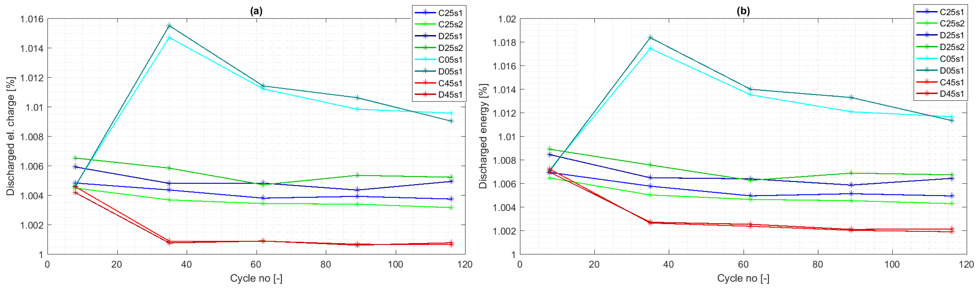
4. Experiment Results

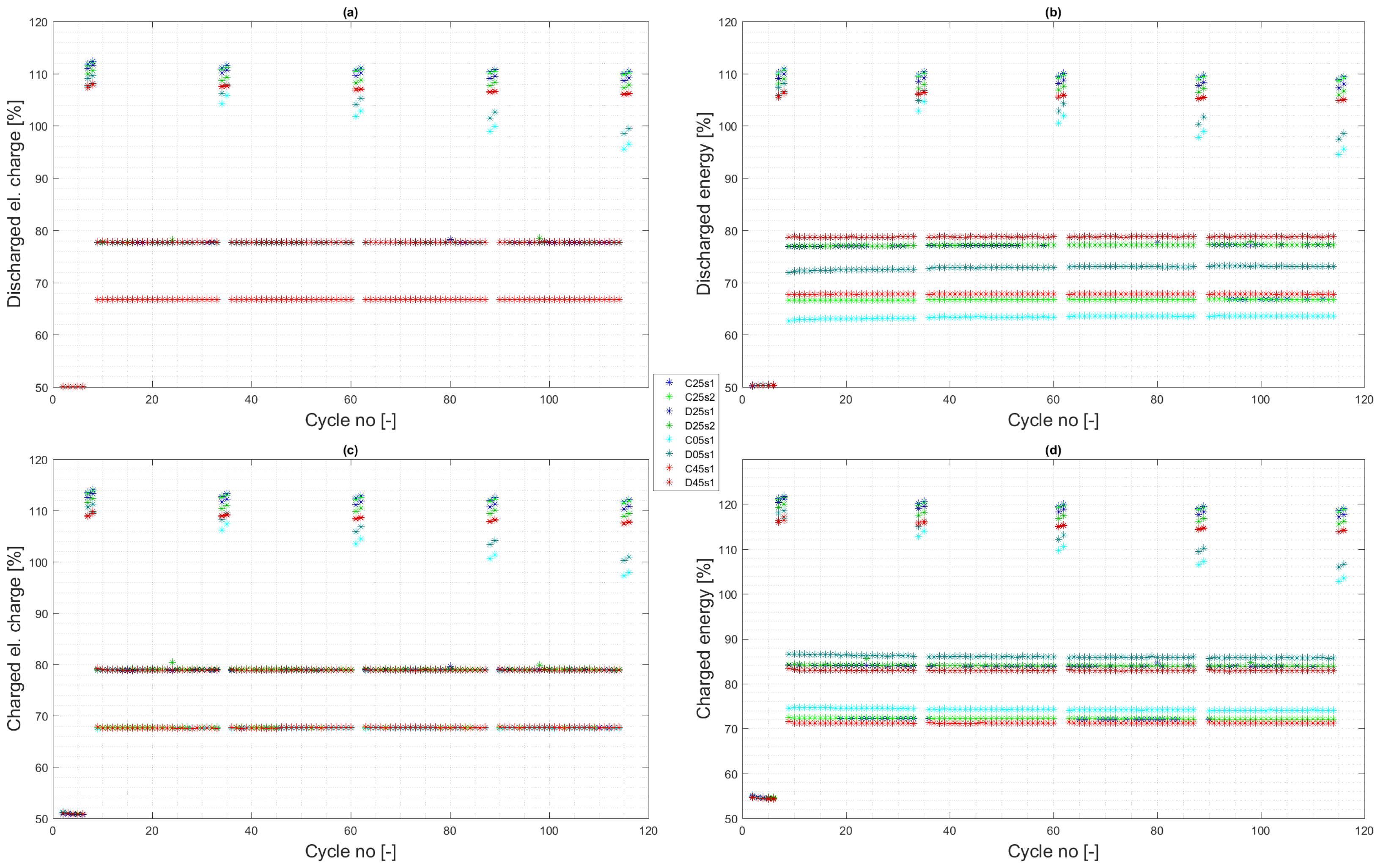
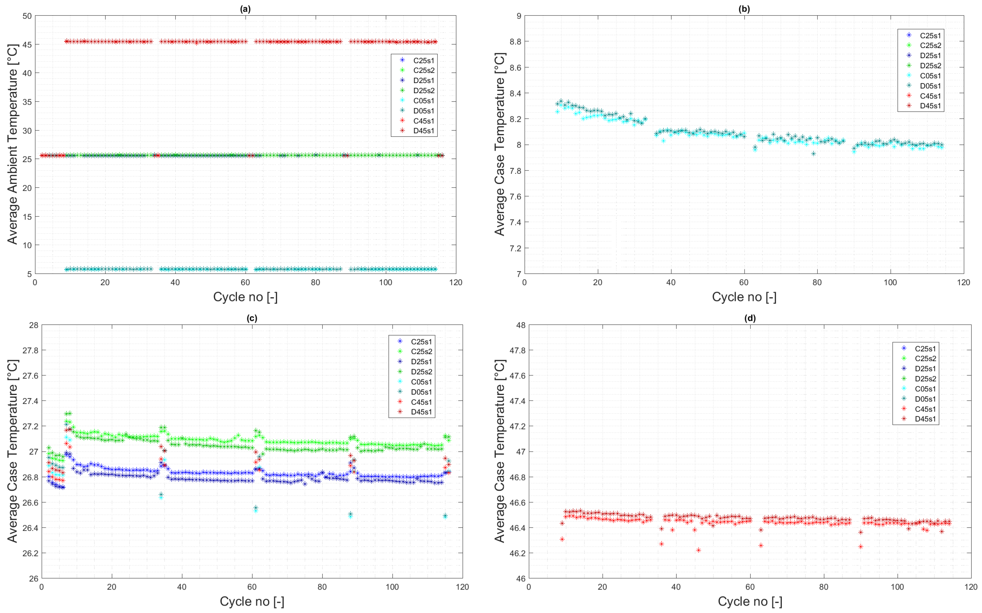
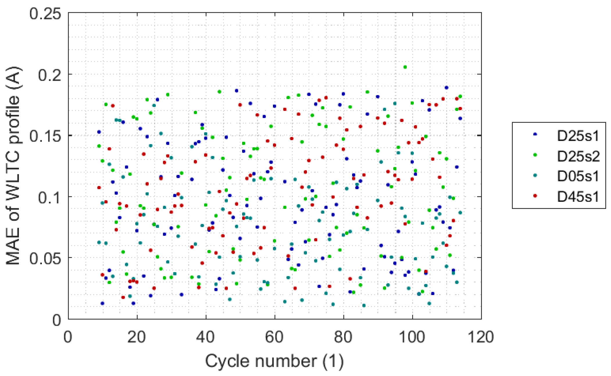
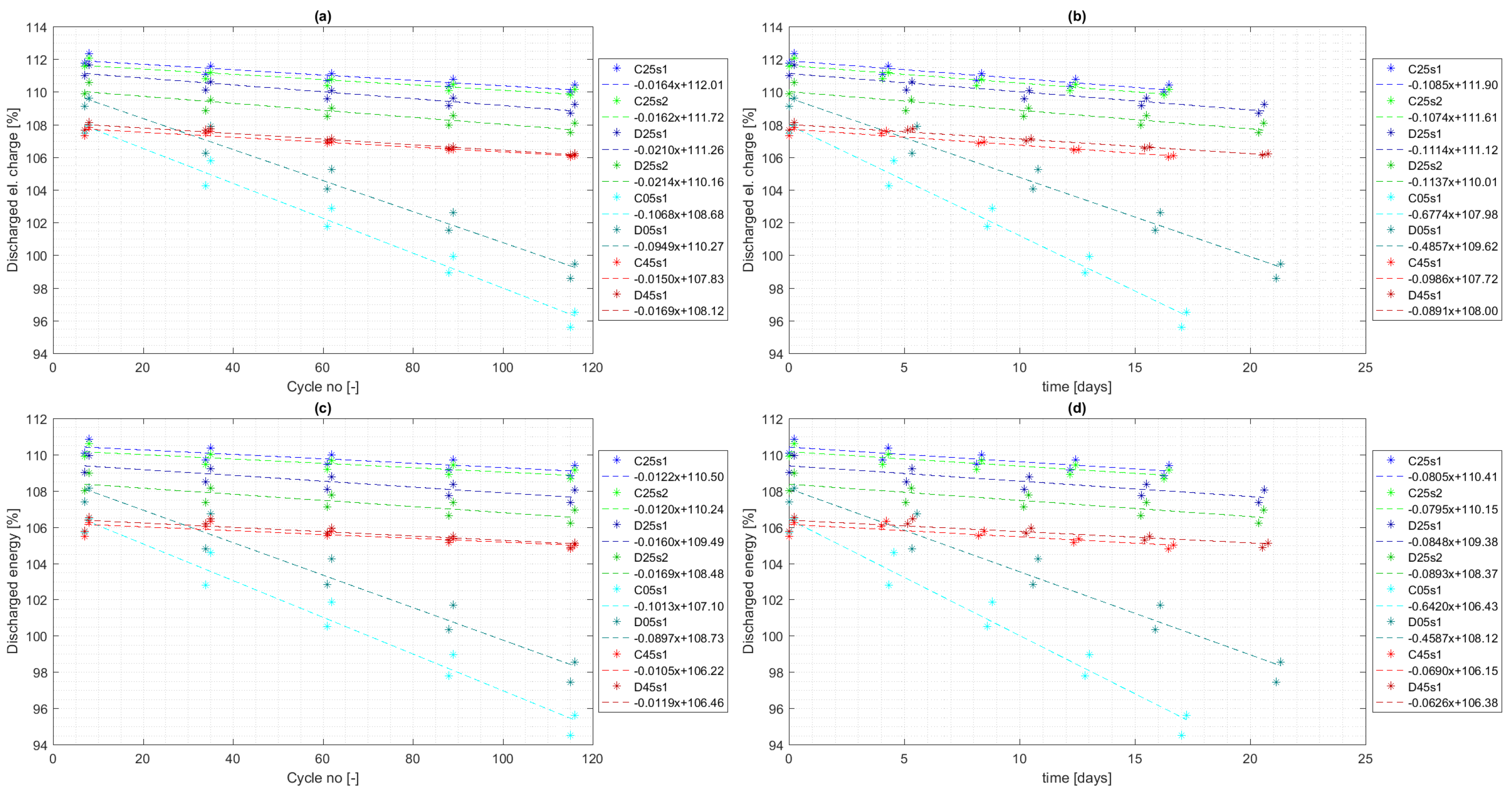
4.1. Experiment Validity Verification

Figure 6 shows measured values throughout all the measured samples for electric charge and energy. Three anomalies are apparent in the figure of electrical charge for D25s2 at cycles 24 and 98 and for D25s1 at cycle 80. They are all caused by interruption of the measurement after completed cycle due to technical circumstances.

Figure 7 shows measured values throughout all the measured samples for Coulombic and energy efficiency. Again, there is an apparent drop for D25s2 at cycle 24, otherwise it can be observed, that for normal cycles (excluding the initial and the formatting cycles) the Coulombic efficiency is between 98 and 99% and varies around the tests of capacity, where cycling operation conditions are changing. Coulombic efficiency does not much depend on discharge mode and although its values are slightly lower for drive cycle discharge mode, the differences from CC discharge mode are negligible. There is no apparent dependency of Coulombic efficiency on temperature. Energy efficiency depends strongly on temperature: the lower the temperature is, the stronger it also depends on the discharge mode. The similarity of the results of C25s1/C25s2 and D25s1/D25s2 is sufficient, which enables only one sample per temperature and discharge mode for the remaining studied temperatures. The sudden drop in energy efficiency for C45s1 at cycle 45 is caused by interruption of the measurement due to technical circumstances within charging cycle 45. All the other interruptions mentioned above occurred always after finishing cycle charging. The gradual increase in energy efficiency is apparent especially for both samples at temperature 5 °C. Figure 8 supports that phenomenon, as for the higher cycle number, the shape of charge and discharge voltages becomes narrower and the amount of electric charge transported within CV mode lessens compared to the low cycle number. Point (b) of Figure 7 shows a gradual increase in the end discharging voltages of all individual 116 cycles, which corresponds to the narrower shape of the discharge/charge characteristic in sub-figure (a) of Figure 8. The phenomenons noticeable in Figure 7 and Figure 8 correspond to capacity recuperation described in [29], which explains the step growth of energy efficiency and end discharge voltage occurring immediately after the two consecutive capacity tests.

Figure 9 illustrates dV/dQ curves for all the samples used for cycle aging discharged in CC mode. Again, there is negligible difference between C25s1 and C25s2. As for temperature 5 °C, peaks shift before the end of discharging can be observed. As there is a dependency between dV/dQ shape and SoC [30], it seems for the temperature 5 °C, that during each normal cycles of the first metacycle, that SoC operation interval floated upwards, while for the other metacycles it stays steady during the whole metacycle. This corresponds to the growth of energy efficiency apparent in Figure 7, which is increasing during the whole first metacycle, while for the following metacycles it always grows, but stays steady during the metacycle itself.

Figure 10 shows measured values throughout all of the samples for the average values of ambient and cell case temperatures. As for ambient temperature, positive offsets of temperature 0.75, 0.60 and 0.4 °C can be observed for set temperatures 5, 25 and 45 °C, respectively. These offsets are slightly higher for drive cycle discharge mode, but the difference between the two modes is not higher than 0.05 °C. Concerning case temperatures, positive offsets of temperature around 3.2, 2.0 and 1.5 °C can be observed for set temperatures 5, 25 and 45 °C, respectively. One can see for temperature 25 °C, that pairs C25s1&D25s1 and C25s2&D25s2 are similar to each other, which is caused by similar values of internal resistances apparent in Table 3. For the other temperatures, internal resistances of samples for both discharge modes are almost identical, thus the temperatures of both samples are almost the same, the differences are not higher than 0.05 °C.

Four consecutive WLTC Class 3b drive cycle profiles adapted to battery composed of LiFeYPO₄ 40Ah cells were used for drive cycle mode discharging, which is described in detail above in Section 2.4. The required current profile imposed to the measured cell was compared to the real measured current profile for all the measured drive cycles discharging and all the appropriate cells and their mean absolute error (MAE) was evaluated for verification purposes. The mean value of MAE for all the cycles and samples is 0.095 A, the maximum value is 0.205 A. All the MAE values are apparent in Figure 11.

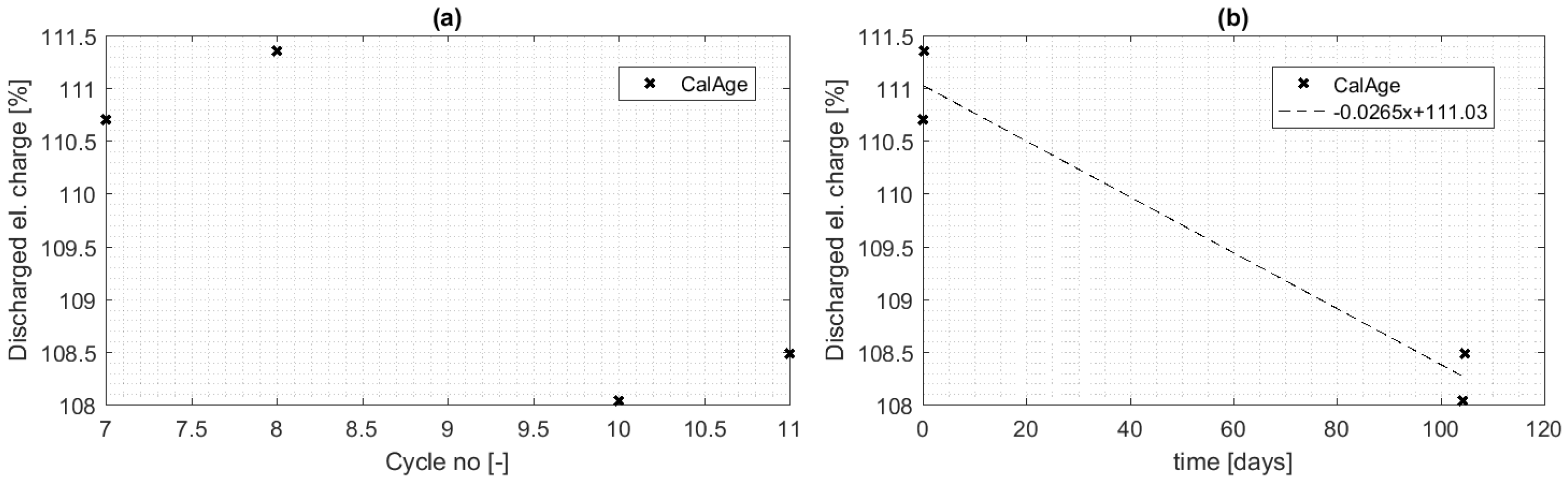
4.2. Calendar Aging

Figure 12 shows results of the CalAge cell used for calendar aging. This cell was placed inside the incubator with set temperature of 25 °C for the whole duration of performing cycle aging tests for the cells C25s1, C25s2, D25s1 and D25s2 in an open circuit state.

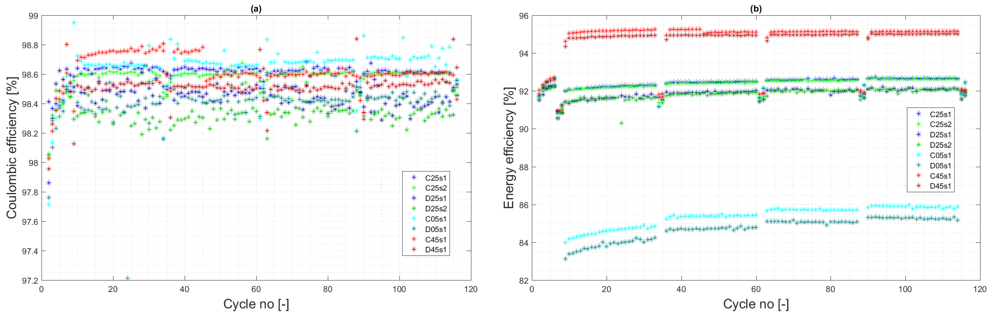
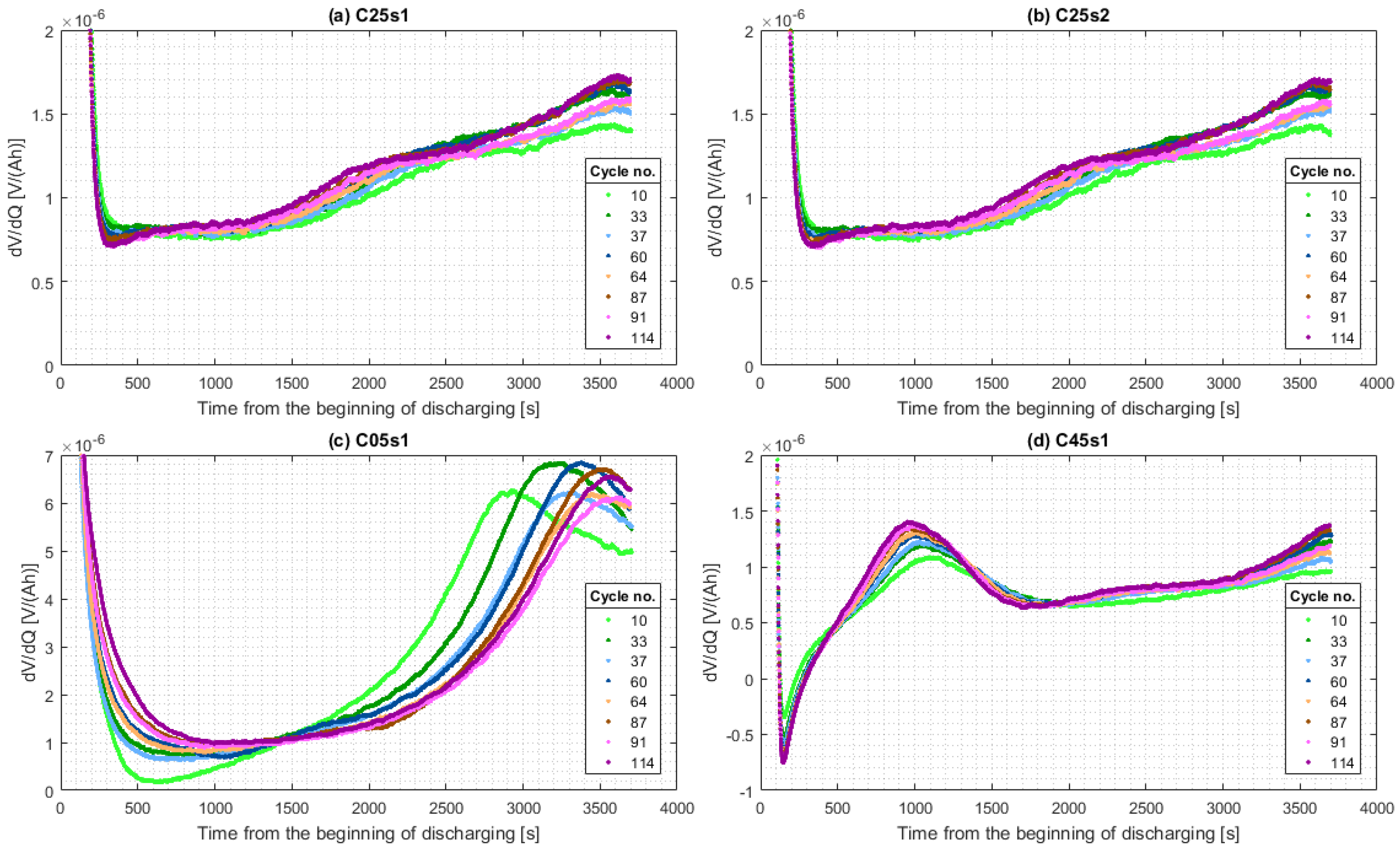
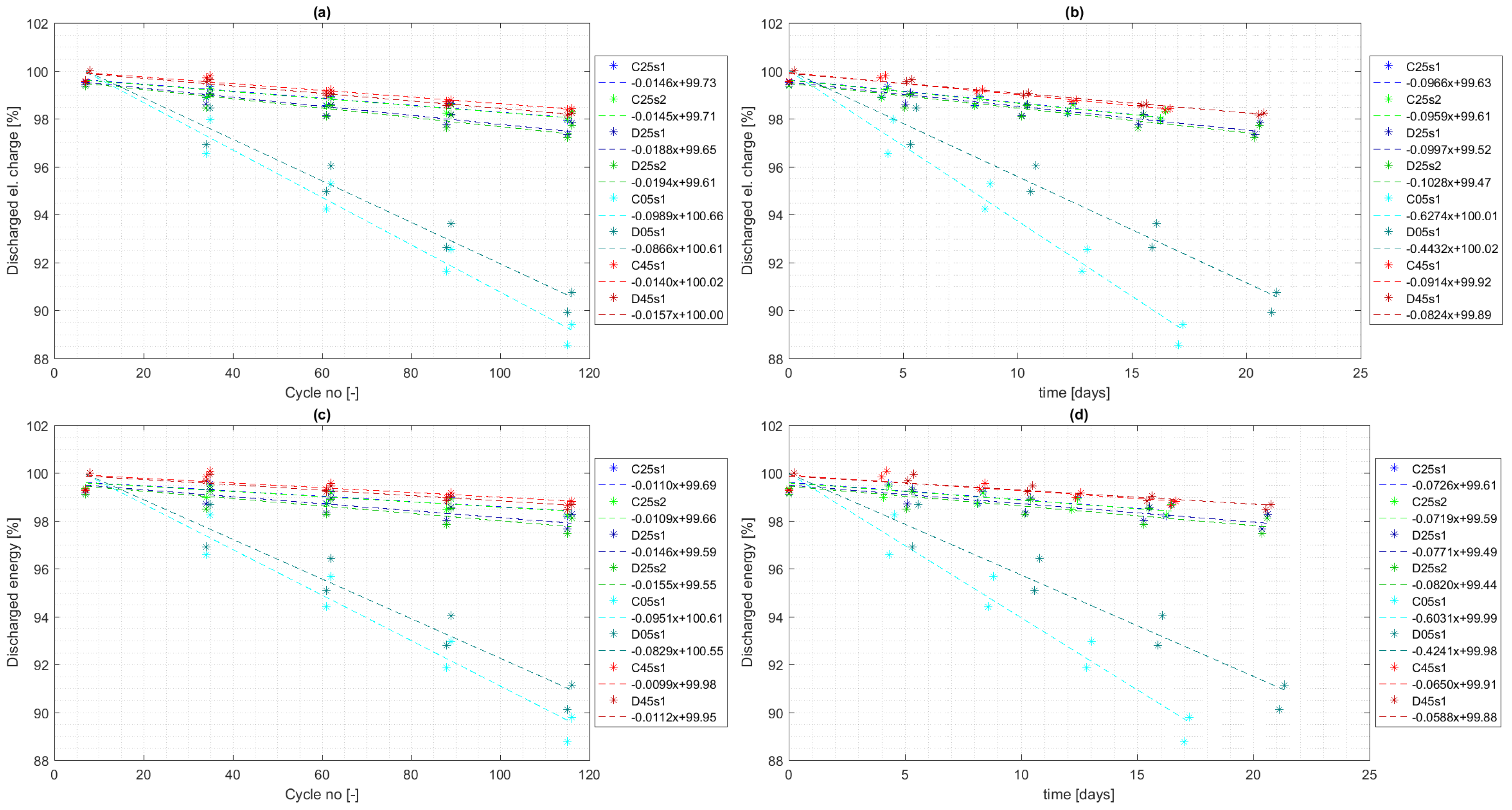
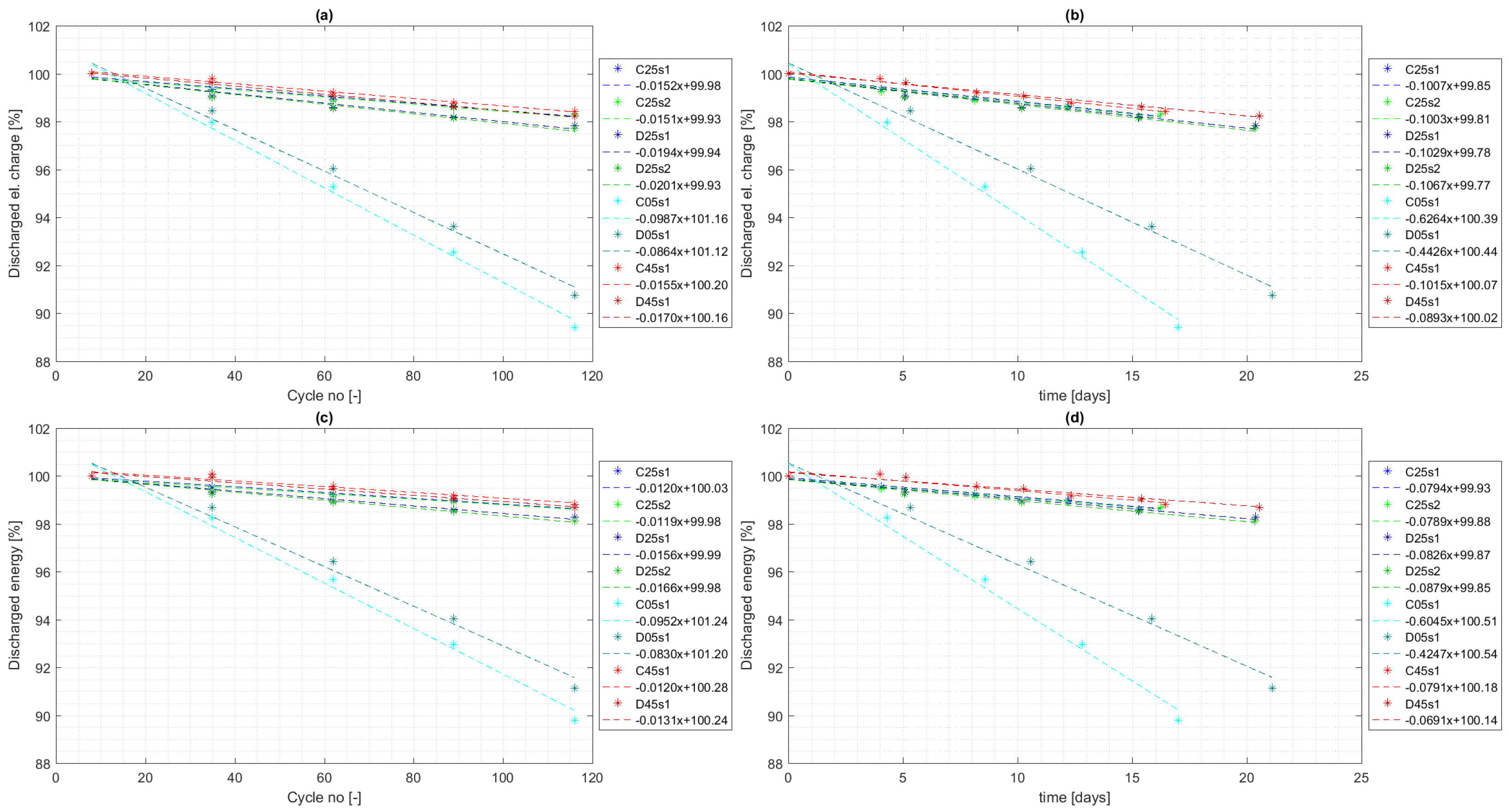
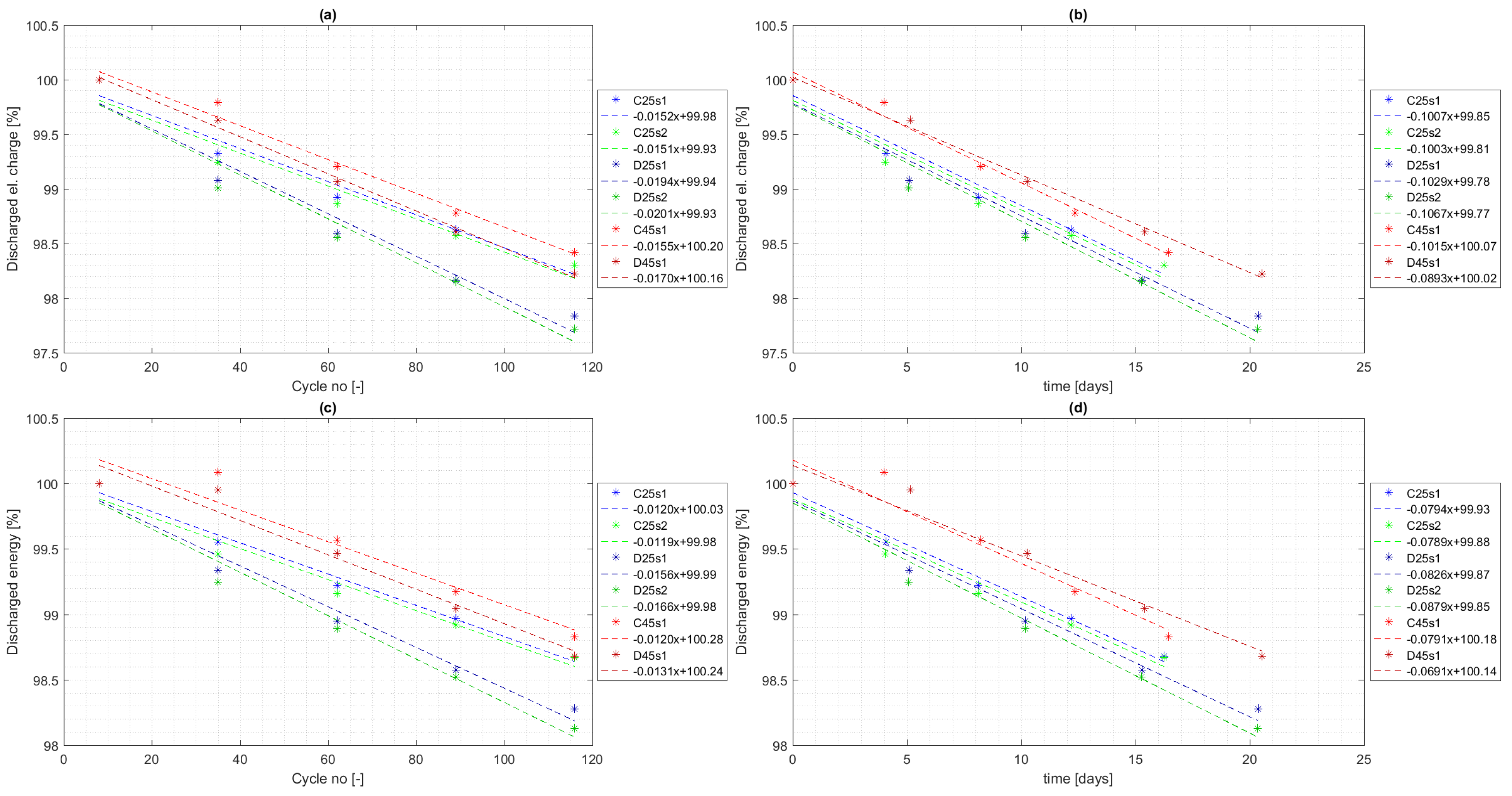
4.3. Cycle Aging

Raw data were corrected to eliminate the influence of above mentioned measurement interruptions. The correction was based on the fact, that the cells were in open circuit state during interruption, so Calendar aging capacity fade −0.027453%/day was compensated for all the capacity tests following the respective interruption. Additionally, the time was lessened by exact duration of each interruption. Time dependencies in Figure 13, Figure 14, Figure 15 and Figure 16 show proportional duration of drive cycle discharging cycles compared to CC discharging cycles.

Results of all the cells used for cycle aging are shown in Figure 13. Capacity increase in the second of the two consecutive capacity tests is in accordance with [29]. Values normalized to the second cycle of the first two consecutive capacity tests (cycle no. 8) are presented in Figure 14. The results of capacity and discharged energy considering only the second one from the two consecutive capacity tests are shown in Figure 15.

As the results shown in Figure 15 are of significant difference between 5 °C and the other temperatures, Figure 16 shows results for 25 and 45 °C only.

Figure 17 shows ratios of the capacity and energy, respectively, of two consecutive capacity tests. This ratio depends on temperature of normal cycles. It is clearly seen, that the first capacity test was influenced by the temperature of previous normal cycle. Initial value of the ratio is similar for all the samples, as the formatting was performed at 25 °C for all the samples in the same way. Normal cycles under different temperatures started after the first two consecutive capacity tests. This justifies performing two consecutive capacity tests aiming to eliminate dependency of capacity fade on temperature of normal cycles.

Table 4. Linear regression coefficients of capacity depending on cycle no. (denoted as /C) or time (denoted as /T) in days considering the second capacity test (denoted as S) or all the capacity tests (denoted as A) for individual samples.

Sample	Cap/C S	Cap/C A	Cap/T S	Cap/T A
C25s1	$-0.0152$	$-0.0146$	$-0.1007$	$-0.0966$
C25s2	$-0.0151$	$-0.0145$	$-0.1003$	$-0.0959$
D25s1	$-0.0194$	$-0.0188$	$-0.1029$	$-0.0997$
D25s2	$-0.0201$	$-0.0194$	$-0.1067$	$-0.1028$
C05s1	$-0.0987$	$-0.0989$	$-0.6264$	$-0.6274$
D05s1	$-0.0864$	$-0.0866$	$-0.4426$	$-0.4432$
C45s1	$-0.0155$	$-0.0140$	$-0.1015$	$-0.0914$
D45s1	$-0.0170$	$-0.0157$	$-0.0893$	$-0.0824$

and

Table 5. Linear regression coefficients of energy depending on cycle no. (denoted as /C) or time (denoted as /T) in days considering the second capacity test (denoted as S) or all the capacity tests (denoted as A) for individual samples.

Sample	Ene/C S	Ene/C A	Ene/T S	Ene/T A
C25s1	$-0.0120$	$-0.0110$	$-0.0794$	$-0.0726$
C25s2	$-0.0119$	$-0.0109$	$-0.0789$	$-0.0719$
D25s1	$-0.0156$	$-0.0146$	$-0.0826$	$-0.0771$
D25s2	$-0.0166$	$-0.0155$	$-0.0879$	$-0.0820$
C05s1	$-0.0952$	$-0.0951$	$-0.6045$	$-0.6031$
D05s1	$-0.0830$	$-0.0829$	$-0.4247$	$-0.4241$
C45s1	$-0.0120$	$-0.0099$	$-0.0791$	$-0.0650$
D45s1	$-0.0131$	$-0.0112$	$-0.0691$	$-0.0588$

show the resulting regression coefficients of measured capacity and energy, respectively, for capacity test cycles.

Results of capacity fade per cycle for drive cycle discharge cycles cells compared to CC discharge cycles cells evaluated based on second capacity tests show:

• 30.4% increase in capacity fade at temperature 25 °C ($-0.0198$ vs. $-0.0152\%$ per cycle);
• 12.5% decrease in capacity fade at temperature 5 °C ($-0.0864$ vs. $-0.0987\%$ per cycle);
• 9.7% increase in capacity fade at temperature 45 °C ($-0.0170$ vs. $-0.0155\%$ per cycle).

Results of capacity fade per day for drive cycle discharge cycles cells compared to CC discharge cycles cells evaluated based on second capacity tests show:

• 4.3% increase in capacity fade at temperature 25 °C ($-0.1048$ vs. $-0.1005\%$ per cycle);
• 29.3% decrease in capacity fade at temperature 5 °C ($-0.4426$ vs. $-0.6264\%$ per cycle);
• 12.0% decrease in capacity fade at temperature 45 °C ($-0.0893$ vs. $-0.1015\%$ per cycle).

The results at 25 °C show, that there is 30.4% higher capacity fade for drive cycle discharge cycles depending on cycle number, but when compared in time, the capacity fade difference 4.3% is quite similar for both cycle modes. Complete measurement of 116 cycles of drive cycle discharge cycles took 26.7% longer than complete measurement of CC discharge cycles. Electric charge discharged during normal cycles was 16.5% higher on average and electric charge charged during normal cycles was 16.7% higher on average due to WLTC waveform character.

The results at temperature 5 °C show a 12.5% decrease in cycle capacity fade and a 29.3% decrease in capacity fade with respect to time. The complete measurement of 116 cycles of drive cycle discharge cycles took 23.7% longer than the complete measurement of CC discharge cycles. Electric charge ratios were the same as for 25 °C.

The results at temperature 45 °C show a 9.7% increase in cycle capacity fade and a 12.0% decrease in capacity fade with respect to time. The complete measurement of 116 cycles of drive cycle discharge cycles took 24.6% longer than the complete measurement of CC discharge cycles. Electric charge ratios were the same as for 25 °C.

5. Aging Simulation

As previously mentioned, calendar and cycle aging are complex aging phenomena in a battery cell which can have negative impacts on the performance of the battery. One of the two principle effects of battery aging identified by [31] is capacity fade which gradually, among others, reduces the reachable range of the BEVs through their life cycles. Various battery degradation mechanisms such as the electrolyte decomposition, solvent co-intercalation, gas evolution and others lead to capacity fade [1]. However, some of them have been accepted by researchers as the dominant aging mechanisms. These mechanisms were calibrated on a single lithium-ion cell model within the simulation tool GT-AutoLion and their calibration processes are further described in Section 5.2.

5.1. Concise Description of P2D Model

GT-AutoLion is a part of industry-leading simulation tool GT-SUITE. GT-Autolion follows the principles of the P2D model for lithium-ion batteries. The P2D model is based on the work of John Newman and captures the electrochemical reactions occurring inside a Li-ion cell to predict metrics such as the terminal voltage, current, power, heat rejection, and the amount of lithium throughout the cell [32]. As shown in Figure 18, the model discretizes the lithium-ion cells using the finite control volume approach. The cathode, anode, and separator in the direction of “thickness”. Additionally, in each control volume of the cathode and anode, there is one spherical representation of active material, each of which are discretized in constant volumes in the radial direction based of Fick’s law of diffusion for the active material concentration.

5.2. P2D Model Calibration

When it comes to aging modeling in GT-AutoLion, users have the ability to model the film layer growth of the active material, both the cathodic film layer growth and the anodic film layer growth, lithium-plating, as well as active material cracking or active material isolation. In this paper, only certain aging mechanisms are considered with respect to the experiment as described in Section 5.2.1 and Section 5.2.2. Calibrations were performed on the single LFP/graphite cell model, which is based on the previous result [19].

5.2.1. Calendar Aging

SEI Layer Growth

Calendar aging data are often used to calibrate the film growth aging mechanisms in both the cathode and anode. However, the passivation layer in lithium-ion cells with graphitic anodes, referred to as the solid electrolyte interphase (SEI) layer [34], produced by parasitic reactions at the negative electrode/electrolyte interface can be considered as the dominant aging factor during battery storage leading to an irreversible loss of lithium inventory (LLI) [35,36,37]. Ref. [38] revealed that the main cause of capacity fade for different cathode cell types with the graphitic anode is due to low anode potentials, where the graphite anode is lithiated more than 50% accelerating the LLI. They also revealed that the Fe dissolution represents only a minor aging mechanism during cell storage. Moreover, Fe dissolution and its precipitation on the anode is exhibited only at elevated storage temperatures [39,40]. Ref. [40] studied aging of LiFePO4/graphite cells during long-term storage under different temperature conditions and states of charge. They found that the olivine-type structure of the cathode is maintained even with long-term storage at elevated temperature of 55 °C and at 100% SoC. Moreover, crystallization properties of LiFePO4 have no influence at these conditions. They concluded that the main aging factor arises from side reactions taking place at the graphitic anode. Therefore, the SEI layer growth on the anode was only considered, which always results in capacity fade and resistance growth [41], even when there is no current going through a cell.

Governing Equations

To ensure an accurate simulation, parameter identification plays a key role in the calibration of a P2D model. There have been a few published studies that distinguish dominant control mechanisms in the SEI growth rate, namely, the diffusion of the solvent molecules across the SEI [42,43] or the kinetics of the side reaction occurring at the graphite/SEI interface [44,45]. This paper takes into account both mechanisms. Thus, the SEI layer growth model was calibrated through the kinetic growth parameters, specifically the diffusivity of ethylene carbonate (EC) through the existing SEI layer and the kinetic rate coefficient for the electrochemical side reactions responsible for the SEI layer growth. During the SEI layer growth reaction, EC diffuses through the existing SEI layer, the rate of which is defined by the EC diffusivity. Moreover, side reactions occur which increase the resistivity of the film and decrease the porosity of the anode and add SEI resistance to the system. As mentioned already, only the SEI growth is considered as side reaction occuring at the anode during cell storage, which is described by the following reaction [46]:

$$2{\left({\mathrm{CH}}_2\mathrm{O}\right)}_2\mathrm{CO}+2{\mathrm{e}}^{-}+2{\mathrm{Li}}^{+}\to {\left({\mathrm{CH}}_2{\mathrm{OCO}}_2\mathrm{Li}\right)}_2\downarrow +{\mathrm{C}}_2{\mathrm{H}}_4\uparrow$$

(1)

where the SEI layer is composed of lithium ethylene dicarbonate ${\left({\mathrm{CH}}_2{\mathrm{OCO}}_2\mathrm{Li}\right)}_2$ arises from the reaction of ethylene carbonate ${\left({\mathrm{CH}}_2\mathrm{O}\right)}_2\mathrm{CO}$ with lithium-ions. In that reaction, 3 reactants are consumed. Firstly, the consumption of cyclable lithium-ions causes cell capacity reduction. Secondly, the consumption of electrons manifests as a decrease in Coulombic efficiency below one. Lastly, the solvent consumption makes the electrolyte less conductive. The total current density in the anode is given by:

$$j_{total,anode}=j^{IC}+j_{SEI}$$

(2)

where the $j^{IC}$ is the volumetric intercalation reaction current density taking place at the electrode/electrolyte interface and the $j_{SEI}$ is the side reaction current density. The volumetric intercalation reaction current density $j^{IC}$ is given by the Butler–Volmer Equation [47]:

$$j^{IC}=a_s{i}_0^{IC}\left\{\exp \left[\frac{{\alpha }_{a}F}{R_{u}T}\left(\eta -\frac{R_{SEI}}{a_s}{j}^{Li}\right)\right]-\exp \left[\frac{{\alpha }_{c}F}{R_{u}T}\left(\eta -\frac{R_{SEI}}{a_s}{j}^{Li}\right)\right]\right\}$$

(3)

where $a_s$ is the volume specific reaction surface area, $i_0^{IC}$ is the exchange current density of intercalation reaction, ${\alpha }_a$ and ${\alpha }_c$ are the anodic and cathodic charge transfer coefficients, respectively, F is the Faraday constant, $R_u$ is the universal gas constant, T is the thermodynamic temperature, $\eta$ is the surface over-potential, $R_{SEI}$ is the resistance of the SEI layer and $j^{Li}$ is the reaction current density. The side reaction current density $j_{SEI}$ based on the reaction surface area is described by the following kinetic equations [48]:

$$j_{SEI}=-a_s{i}_{0,SEI}\exp \left(-\frac{{\alpha }_{c,SEI}F}{RT}\left({\varphi }_s-{\varphi }_e-U_{SEI}-\frac{j^{Li}}{a_s}{R}_{SEI}\right)\right),$$

(4)

$$i_{SEI}=\frac{j_{SEI}}{a_s},$$

(5)

where $j_{SEI}$ is the side reaction current density, $a_s$ is the volume specific reaction surface area, $i_{0,SEI}$ is the exchange current density of the side reaction, ${\alpha }_{c,SEI}$ is the charge transfer coefficient, ${\varphi }_s$ is the solid-phase potential, ${\varphi }_e$ is the liquid-phase potential, $U_{SEI}$ is the equilibrium potential, $j^{Li}$ is the total current density of both lithium intercalation/deintercalation and side reactions and $R_{SEI}$ is the resistance of the SEI layer. The exchange current density of the SEI layer growth side reaction $i_{0,SEI}$, which has a first-order dependence on EC concentration at the reaction surface $c_{EC}^s$, is given by [48]

$$i_{0,SEI}=F{k}_{0,SEI}{c}_{EC}^s,$$

(6)

where F is the Faraday constant, $k_{0,SEI}$ is the kinetic rate coefficient of the SEI layer growth side reaction and $c_{EC}^s$ is the EC concentration at the reaction surface. In lithium-ion cells, especially in electrolytes for LFP/graphite based cells [37], EC is a part of the electrolyte solution and its concentration in it is significant with appreciable effect on the SEI layer growth [42]. In order to promote the SEI layer growth side reaction, the EC diffusion through the existing SEI layer reaching graphite/SEI interface has to be realized [42,48]. Therefore, GT-AutoLion defines a diffusivity of the EC through the SEI layer denoted as $D_{EC}$. The existing SEI layer is a torturous path, thus GT-AutoLion calculates an effective EC diffusivity by following a Bruggeman relationship where the Bruggeman exponent, n, is assumed to be 1.5 [48]

$$D_{EC}^{eff}=D_{EC}{\left({\epsilon }_{SEI}\right)}^n,$$

(7)

where ${\epsilon }_{SEI}$ is the porosity of the existing SEI layer. The material balance for the EC diffusion in the SEI porous layer is given by [48]

$$\frac{\partial c_{EC}}{\partial t}=D_{EC}^{eff}\frac{{\partial }^2{c}_{EC}}{\partial r^2}.$$

(8)

By solving the Equations (7) and (8), the SEI layer thickness denoted as ${\delta }_{SEI}$ will increase according to the following equation [48]:

$$\frac{d{\delta }_{SEI}}{dt}=-\frac{i_{SEI}}{2F}\frac{M_{SEI}}{{\rho }_{SEI}}$$

(9)

where $M_{SEI}$ is the molecular weight of the SEI layer and ${\rho }_{SEI}$ is the density of the SEI layer. The resistance of the SEI layer can be calculated by [48]:

$$R_{SEI}=\frac{{\delta }_{SEI}}{{\kappa }_{SEI}^{\mathit{eff}}}$$

(10)

where ${\kappa }_{SEI}^{\mathit{eff}}$ is the effective conductivity of the electrolyte through the porous SEI layer. The effective conductivity ${\kappa }_{SEI}^{eff}$ is corrected with the following Bruggeman relationship due to a tortuous path through the porous SEI layer [48]:

$${\kappa }_{SEI}^{\mathit{eff}}={\kappa }_{SEI}{\left({ϵ}_{SEI}\right)}^n$$

(11)

where ${\kappa }_{SEI}$ is the ionic conductivity of the film and ${ϵ}_{SEI}$ is the volume fraction of SEI in the film. SEI layer thickening causes the lowering of anode porosity leading to the poorer Li-ion transport properties, and thus increased resistance of the cell. In GT-AutoLion, the relation between the SEI layer thickening and anode porosity is calculated according to following equation [48]:

$$\frac{dϵ}{dt}=-a_s\frac{d\left({\delta }_{SEI}\right)}{dt}$$

(12)

where $ϵ$ is the porosity of the anode. The kinetic rate coefficient of the SEI layer growth side reaction $k_{0,SEI}$ and the EC diffusivity $D_{EC}$ have been chosen as calibrated parameters. These parameters represent temperature-dependent physical-chemical properties which are described by the modified Arrhenius equation to account how they vary with temperature [48,49]

$$\varphi ={\varphi }_{ref}·\exp \left[\frac{E_{act,\varphi }}{R}·\left(\frac{1}{T_{ref}}-\frac{1}{T}\right)\right],$$

(13)

where $\varphi$ represents a value of a physical-chemical property (the kinetic rate coefficient or the effective diffusivity in that case) at any temperature T, ${\varphi }_{ref}$ is a value of that physicochemical property at the reference temperature $T_{ref}$, $E_{Act}$ is the corresponding activation energy and R is the gas constant. For these Arrhenius objects, we have parameterized the value of the property at reference temperature ${\varphi }_{ref}$ and activation energy $E_{Act}$. Remaining parameters of the anode SEI layer growth model were assumed to be constant. The parameter values were derived from the pre-fills of the GT-AutoLion’s large database of various anode, cathode, and electrolyte material properties and for clear arrangement are listed in

Table 6. Considered parameters of the calibrated anode SEI layer growth model at temperature 25 °C. c: constant parameter; f: fitted parameter to experimental data; es: estimated value.

Parameter Symbol	$\mathbf{Lower}$	$\mathbf{Initial}$	$\mathbf{Upper}$	$\mathbf{Unit}$
${\varphi }_{re{f}_{ECDiff}}^f$	$5·{10}^{-20es}$	$1·{10}^{-19es}$	$2·{10}^{-19es}$	$({\mathrm{m}}^2/\mathrm{s})$
$E_{Ac{t}_{ECDiff}}^f$	$5.6·{10}^{4es}$	$7·{10}^{4es}$	$9.8·{10}^{4es}$	$(\mathrm{J}/\mathrm{mol})$
${\varphi }_{re{f}_{SEIRate}}^f$	$7.5·{10}^{-17es}$	$1.5·{10}^{-16es}$	$3·{10}^{-16es}$	$(\mathrm{m}/\mathrm{s})$
$E_{Ac{t}_{SEIRate}}^f$	$4.8·{10}^{4es}$	$6·{10}^{4es}$	$8.4·{10}^{4es}$	$(\mathrm{J}/\mathrm{mol})$
$U_{SEI}^c$	−	$0.4$ [44,50,51]	−	$\left(\mathrm{V}\right)$
${\alpha }_{c,SEI}^c$	−	$0.5$ [44,52,53]	−	$(-)$
$M_{SEI}^c$	−	162 [54]	−	$(\mathrm{g}/\mathrm{mol})$
${\rho }_{SEI}^c$	−	$1.69$ [54]	−	$(\mathrm{g}/{\mathrm{cm}}^3)$
${\epsilon }_{SEI}^c$	−	$0.05$ [51,52]	−	$(-)$

and

Table 7. Description of the parameters from Table 6.

Parameter Symbol	$\mathbf{Description}$
${\varphi }_{re{f}_{ECDiff}}^f$	$\mathrm{Value}\mathrm{of}\mathrm{the}\mathrm{EC}\mathrm{diffusivity}$
$E_{Ac{t}_{ECDiff}}^f$	$\mathrm{Activation}\mathrm{energy}\mathrm{for}\mathrm{the}\mathrm{EC}\mathrm{diffusivity}$
${\varphi }_{re{f}_{SEIRate}}^f$	$\mathrm{Value}\mathrm{of}\mathrm{the}\mathrm{rate}\mathrm{coefficient}$
$E_{Ac{t}_{SEIRate}}^f$	$\mathrm{Activation}\mathrm{energy}\mathrm{for}\mathrm{the}\mathrm{rate}\mathrm{coefficient}$
$U_{SEI}^c$	$\mathrm{Equilibrium}\mathrm{potential}\mathrm{of}\mathrm{the}\mathrm{SEI}$
${\alpha }_{c,SEI}^c$	$\mathrm{Charge}\mathrm{transfer}\mathrm{coefficient}\mathrm{of}\mathrm{the}\mathrm{SEI}$
$M_{SEI}^c$	$\mathrm{Molecular}\mathrm{weight}\mathrm{of}\mathrm{the}\mathrm{SEI}$
${\rho }_{SEI}^c$	$\mathrm{Density}\mathrm{of}\mathrm{the}\mathrm{SEI}$
${\epsilon }_{SEI}^c$	$\mathrm{Porosity}\mathrm{of}\mathrm{the}\mathrm{SEI}$

. Used values for the constant parameters, namely, the $U_{SEI}$, ${\alpha }_{SEI}$, $M_{SEI}$, ${\rho }_{SEI}$ and ${\epsilon }_{SEI}$ can also be find in references stated in Table 6. Initial values or “guesses” of the calibrated parameters were estimated as starting points for the optimization procedure along with their estimated lower and upper threshold values.

Optimization Procedure

The optimization procedure itself was set up in the GT-AutoLion’s Integrated Design Optimizer. The Integrated Design Optimizer is an advanced optimization toolbox that enables users to either optimize parameters for a certain design goal or (in this case) reverse engineer systems by varying unknown parameters to match experimental data (by minimizing the error between simulation and experimental results). It contains several pre-defined and pre-coded optimization routines that allow users to vary any number of parameters in order to run single objective or multi-objective optimization routines that can even do cross-case optimization routines. The goal of this and most optimization routines is to select a “response” or “result” and either minimize it, maximize it, or target a specific value for it. The optimizer’s goal has been to minimize the RMS error (RMSE) by varying the unknown parameters or “factors”. The factors that are varied are the parameters required to be essential to matching the cell’s SoH. The factors varied slightly around the initial guesses set for each parameter.

The optimizer provides deterministic search algorithms as well as evolutionary search algorithms for optimization routines. In this stage, by using the “Accelerated GA”, an advanced genetic algorithm that incorporates meta-modeling between each generation, (essentially a “survival of the fittest”) it is possible to vary these factors to converge on optimized values which help match the experimental and simulated data. RMSE between simulated and experimental SoH of the cells were selected as the optimization criterion. It is worth pointing out that the RMSE was calculated only for the time-stamps of performed capacity tests. For that case, there were two time-steps, specifically at the beginning and at the end of the calendar aging test. By varying the fitted parameters slightly around the initial values within the thresholds defined in Table 6, specifically the EC diffusivity and the film growth rate, the design optimizer minimized the RMSE.

5.2.2. Cycle Aging

Active Material Isolation

After calibrating the model for calendar aging, this model can then be further built upon using cycle aging data in order to calibrate the active material isolation models in GT-AutoLion and potentially lithium-plating. During this step, the calibrated SEI film growth model on the anode is assumed to be pre-calibrated. Owing to the the fact, that the lithium-plating results in capacity fade and resistance growth primarily during periods of high charging current or standard charging current at low temperatures and long-term cycling [55], lithium-plating was neglected in this paper. The active material isolation model results in capacity fade and resistance growth only when current is going through. During active material isolation, or as it is also known, active material cracking, the intercalation and deintercalation of lithium ions can cause mechanical stresses on active material crystalline structure, which can induce cracking. In this paper, only active material isolation on the anode was calibrated.

Governing Equation

Loss of active material at the anode was modeled according to work in [56], in which the rate of isolation at the anode is implemented by the following empirical relationship:

$$\frac{d{ϵ}_{-}}{dt}=(C_1\left(T\right)|i_{-}|+C_2\left(T\right)\sqrt{|i_{-}|})f\left(x\right),$$

(14)

where ${ϵ}_{-}$ is the volume fraction of active material in the anode, $i_{-}$ is the current density at the anode (per unit of active surface area), $C_1\left(T\right)$ is a linear term, $C_2\left(T\right)$ is a square root term and $f\left(x\right)$ is a stoichiometry dependent coefficient. The terms $C_1\left(T\right)$ and $C_2\left(T\right)$ are temperature dependent and the stoichiometry dependent coefficient represents the empirical function of the lithium content described in detail elsewhere [56]. This function is used as a weighting function to account dependency of the rate of loss of anode active material on the lithium content. Based on the simulation results from [56] the empirical model (Equation (14)) matches well with the experimental and the “snapshot”-analysis results for both temperatures and for aging time less than 6 months. The temperature dependent terms $C_1\left(T\right)$ and $C_2\left(T\right)$ and the lithium stoichiometry coefficient $f\left(x\right)$ were fitted. By varying the fitted parameters in the design optimizer by a couple of orders of magnitude, RMSE between experiment and simulation was minimized.

Optimization Procedure

Optimization procedure was different from that one in the calendar aging, since it incorporates two consecutive manually adjustments of the linear ($C_1\left(T\right)$) and square root ($C_2\left(T\right)$) terms to fit the experimental data due to higher computation cost of the optimization. First, the optimization in the design optimizer with the same settings that has been used in the calendar aging optimization incorporating only 27 cycles (25 normal cycles + 2 capacity tests) was performed. Results of that optimization built set of the initial fitted parameter values for each cell sample. Values of the fitted parameters are reported in

Table 8. Fitted parameters $C_1\left(T\right)$, $C_2\left(T\right)$ and $f\left(x\right)$ to experimental data at temperatures 25, 5 and 45 °C from the optimizer.

Sample	${\mathit{C}}_1\left(\mathit{T}\right)$	${\mathit{C}}_2\left(\mathit{T}\right)$	$\mathit{f}\left(\mathit{x}\right)$	$\mathbf{RMSE}$
—	$({\mathrm{m}}^2/\mathrm{A}\text{-}\mathrm{s})$	$(\mathrm{m}/{\mathrm{A}}^{0.5}\text{-}\mathrm{s})$	$(-)$	$(\%)$
C25s1s2	$1.93·{10}^{-8}$	$-6.43·{10}^{-10}$	$0.93$	$0.516$
D25s1s2	$1.89·{10}^{-8}$	$-5.31·{10}^{-9}$	$0.93$	$0.227$
C05s1	$4.70·{10}^{-8}$	$1.96·{10}^{-8}$	$0.93$	$0.871$
D05s1	$3.67·{10}^{-8}$	$2.38·{10}^{-8}$	$0.93$	$0.599$
C45s1	$2.57·{10}^{-8}$	$-1.81·{10}^{-8}$	$0.93$	$0.112$
D45s1	$1.20·{10}^{-8}$	$-1.23·{10}^{-8}$	$0.93$	$0.411$

. Note, that the experimental data used in this optimization for the cell samples aging by the same mode (DrC or CC discharge cycles) and at temperature 25 °C were averaged. Thereafter, based on a sensitivity analysis of the initial fitted parameter values from the optimizer, two manually adjustments were performed. In the first adjustment reported in

Table 9. First adjustment of the parameters $C_1\left(T\right)$ and $C_2\left(T\right)$ to fit the experimental data at temperatures 25, 5 and 45 °C.

Sample	${\mathit{C}}_1\left(\mathit{T}\right)$	${\mathit{C}}_2\left(\mathit{T}\right)$	$\mathit{f}\left(\mathit{x}\right)$	$\mathbf{RMSE}\mathbf{Error}$
—	$({\mathrm{m}}^2/\mathrm{A}\text{-}\mathrm{s})$	$(\mathrm{m}/{\mathrm{A}}^{0.5}\text{-}\mathrm{s})$	$(-)$	$(\%)$
C25s1s2	$1.25·{10}^{-8}$	$-3.50·{10}^{-9}$	$0.93$	$0.205$
D25s1s2	$2.00·{10}^{-8}$	$-5.10·{10}^{-9}$	$0.93$	$0.196$
C05s1	$5.80·{10}^{-8}$	$1.96·{10}^{-8}$	$0.93$	$0.307$
D05s1	$3.00·{10}^{-8}$	$2.49·{10}^{-8}$	$0.93$	$0.383$
C45s1	$2.50·{10}^{-8}$	$-1.81·{10}^{-8}$	$0.93$	$0.100$
D45s1	$2.10·{10}^{-8}$	$-1.50·{10}^{-8}$	$0.93$	$0.075$

, each cell sample parameter except for the parameter $f\left(x\right)$, was adjusted individually for each cell sample. On the contrary, the second adjustment reported in

Table 10. Second adjustment of the parameters $C_1\left(T\right)$ and $C_2\left(T\right)$ to fit the experimental data at temperatures 25, 5 and 45 °C.

Sample	${\mathit{C}}_1\left(\mathit{T}\right)$	${\mathit{C}}_2\left(\mathit{T}\right)$	$\mathit{f}\left(\mathit{x}\right)$	$\mathbf{RMSE}\mathbf{Error}$
—	$({\mathrm{m}}^2/\mathrm{A}\text{-}\mathrm{s})$	$(\mathrm{m}/{\mathrm{A}}^{0.5}\text{-}\mathrm{s})$	$(-)$	$(\%)$
C25s1s2	$1.80·{10}^{-8}$	$-3.61·{10}^{-9}$	$0.93$	$0.198$
D25s1s2	$1.80·{10}^{-8}$	$-3.61·{10}^{-9}$	$0.93$	$0.196$
C05s1	$3.80·{10}^{-8}$	$2.63·{10}^{-8}$	$0.93$	$0.930$
D05s1	$3.80·{10}^{-8}$	$2.63·{10}^{-8}$	$0.93$	$0.929$
C45s1	$2.10·{10}^{-8}$	$-1.46·{10}^{-8}$	$0.93$	$0.103$
D45s1	$2.10·{10}^{-8}$	$-1.46·{10}^{-8}$	$0.93$	$0.106$

fitted the parameter values from the first adjustment together for the cell samples aged at the same temperature. The manual adjustments of the model incorporated all the 108 cycles.

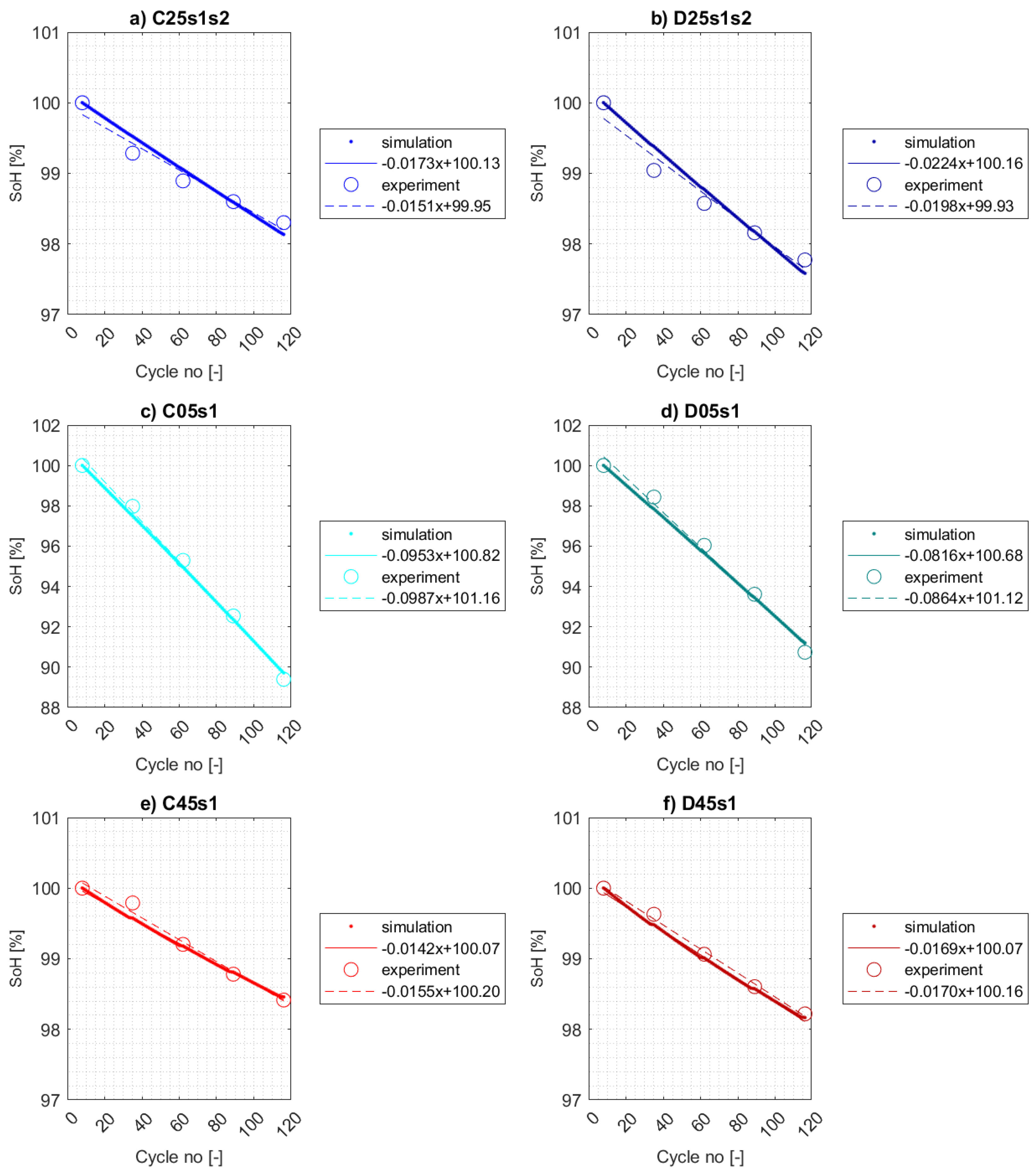
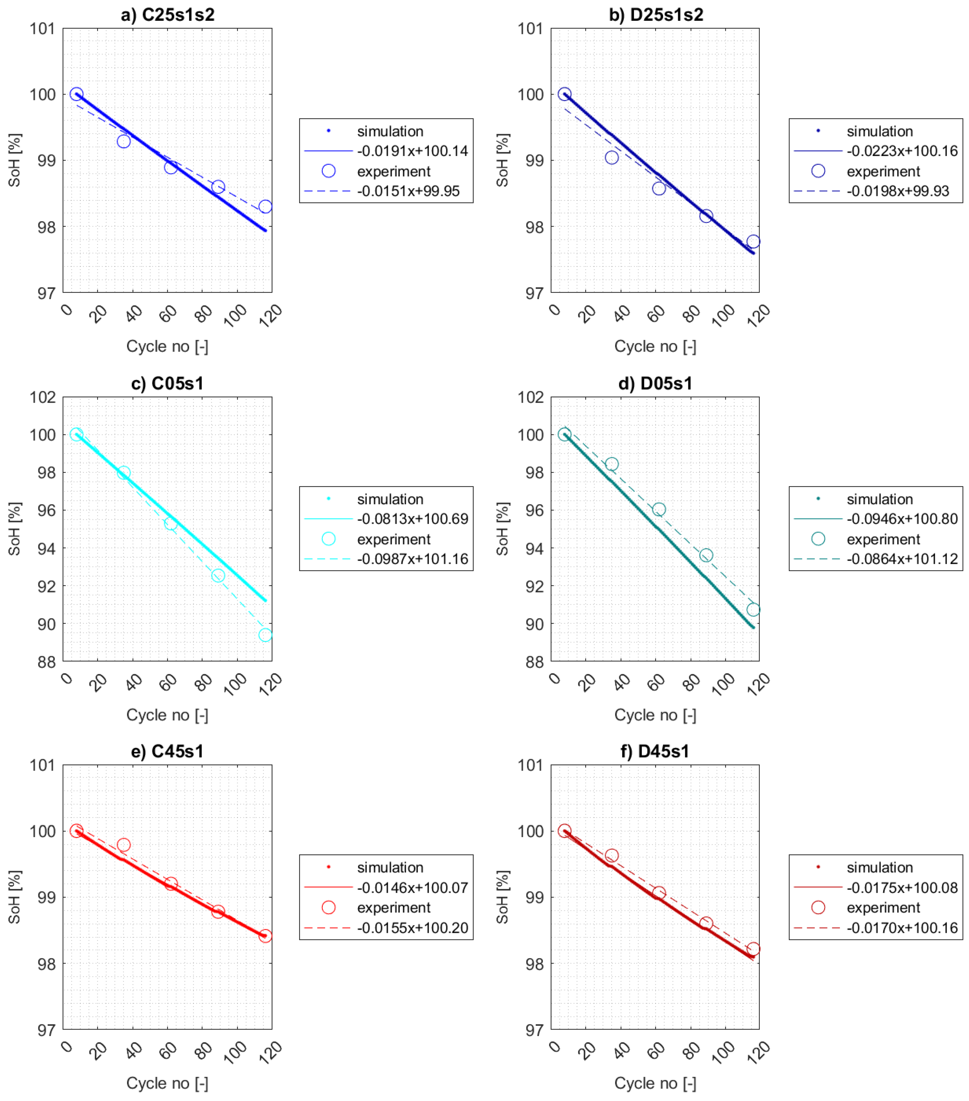
5.3. Simulation Results

5.3.1. Calendar Aging

In total, 241 designs were created with one best design with respect to the minimal value of RMSE, that was $9.573·{10}^{-5}$%. These optimum fitted parameter values of the anode SEI layer growth model are summarized in

Table 11. Fitted parameter values on calendar aging test at temperature 25 °C.

Parameter Symbol	$\mathbf{Fitted}\mathbf{Value}$	$\mathbf{Unit}$
${\varphi }_{re{f}_{ECDiff}}^f$	$1.366·{10}^{-19}$	${\mathrm{m}}^2/\mathrm{s}$
$E_{Ac{t}_{ECDiff}}^f$	$6.897·{10}^4$	$\mathrm{J}/\mathrm{mol}$
${\varphi }_{re{f}_{SEIRate}}^f$	$1.576·{10}^{-16}$	$\mathrm{m}/\mathrm{s}$
$E_{Ac{t}_{SEIRate}}^f$	$5.380·{10}^4$	$\mathrm{J}/\mathrm{mol}$

.

Calendar aging simulation is in a good agreement with the experiment. The fitted value of the EC diffusion coefficient of the solvent through the SEI layer ($1.366·{10}^{-19}$ ${\mathrm{m}}^2/\mathrm{s}$) is in relatively good match with the value reported in [56,57] which was an order of magnitude lower for temperature 25 °C. Additionally, [58] have reported satisfactory simulation results on calendar aging tests, the value of the solvent diffusion coefficient equaled $8.84·{10}^{-20}$${\mathrm{m}}^2/\mathrm{s}$, which is also an order of magnitude lower even at higher storage temperatures.

The fitted value of the rate constant ($1.576·{10}^{-16}$ $\mathrm{m}/\mathrm{s}$) yields worse agreement with the much higher value reported in [56]. Furthermore, [58] have achieved similar value, approximately 2 times higher than in [56]. Nevertheless, [51] have estimated the values of $4.3·{10}^{-16}$ and $2.28·{10}^{-15}$ $\mathrm{m}/\mathrm{s}$ which are almost in conformity with the fitted value. Ref. [45] found that the best fit to the experimental data of the open circuit potential as a function of storage time at storage temperature 25 °C gives the rate constant value of $1.5·{10}^{-18}$ $\mathrm{m}/\mathrm{s}$. However, these values have been estimated for different positive electrode materials. The worse agreement between fitted value and values from other studies might be associated with the different value of the equilibrium potential for the SEI formation used in this paper.

Lastly, the fitted values of the activation energies of both the solvent diffusivity and side reaction rate constant could be considered as good agreement with the manually adjusted values reported in [58].

5.3.2. Cycle aging

The fitted parameter values from the optimization, first and second manually adjustments are presented in Table 8, Table 9 and Table 10, respectively. Results of simulations with adjustment values compared to the experiment are shown in Figure 19 and Figure 20. RMS errors of the manually adjusted fitted parameter values reported in Table 9 indicate, that the model fits in general much better than with the values obtained from the optimization and second adjustment, especially at the aging temperature 5 °C. However, these results lack meaning due to temperature dependency of the fitted parameters across the aging temperatures. The parameter values of both adjustments have the same order of magnitude and also the same signs. They exhibit only slightly variations in their absolute values. These fitted parameters from Equation (14) are hardly provable to be realistic due to the absence of those parameter values in various studies. The adjusted parameter values of the $C_1\left(T\right)$ and $C_2\left(T\right)$ could be directly compared to those ones estimated in [56] only for aging conditions at 25 and 45 °C.

The simulation results reveal that the most remarkable difference between capacity fade at DrC and CC discharge modes occurs at ambient temperature 5 °C. Simulated capacity fade of the cell at CC discharge mode was lower than the experimental one and with exactly opposite capacity fade behavior at DrC discharge mode. Using the simulation results, it can be stated that the correlation between experiment and simulation lies on both, the operating temperature as well as the discharge mode, where its impact on capacity fade is more important at lower temperatures. Three possible reasons could explain the discrepancies between experiment and simulation results at temperature 5 °C:

• Charge consumed in the side reaction at the anode is not counterbalanced by that consumed at the cathode as reported in [56] due to no side reactions occured at the cathode.
• The effects of cycle aging on capacity fade can be superposed by those of calendar aging. Thus, the calibrated SEI layer growth model using experimental data from calendar aging test for 25 °C may be insufficient for calibrating active material isolation model at temperature 5 °C.
• Different behavior of electrolyte model under low operating temperatures.

6. Conclusions

This work shows comparative analysis of LYP/C commercial cells aging for CC discharge cycles and drive cycle discharge cycles testing focused on automotive applications.

Although charge voltage and cut-off currents were the same for all 116 cycles, SoC floating was observed during cycling for both discharge modes, accompanied with slight increase in end discharge voltage and growth of energy efficiency.

Concluding the results for 25 °C, not waveform character, but the amount of electric charge in combination with calendar aging has the most effect on the cycle life, as electric charge increase in drive cycle discharge cycles corresponds to increase in capacity fade per cycle and capacity fade in time is similar for both modes. Simulation results reveals, that when parameters of cell samples pairs used for the two discharging modes were calibrated together, then the simulated results have steeper capacity fade compared to the experimental results for 25 °C, RMSE equals 0.197%. Simulation shows higher capacity fade of drive cycle discharge cycles in case the two discharge modes had equal DoD, which again proves the need of balancing electric charge instead of DoD.

For lower temperature of 5 °C, it seems advantageous for the cycle life, when the cell is discharged dynamically rather than in CC mode. Additionally, calendar aging is not as significant for capacity fade at this temperature. Simulation results show, that the capacity fade is significantly milder for CC discharge cycles and significantly steeper for drive cycle discharge cycles compared to the experiment results, RMSE equals 0.93%. Simulation results do not confirm, that drive cycle discharge cycles are more advantageous than CC discharge cycles in terms of capacity fade. This discrepancy would demand further investigation as well as extension for even lower temperatures.

Results for higher temperature 45 °C are apparently dependent partly on the higher amount of discharged and charged electric charge and partly on the influence of calendar life. Simulated capacity fade corresponds quite well to the experiment, RMSE is 0.105%.

A comparison of meaningful SoH of the simulation results and experimental data is shown in Figure 20. Simulation results are in quite good agreement with the experiments at aging temperatures 25 and 45 °C. As for temperature 5 °C, the simulation results show the important influence of that temperature on estimated capacity fade in both discharge modes with higher aging at DrC mode. The best fit is for temperature 45 °C which has also been reported by [59] using thermally-coupled-electrochemical model intended for the complex drive cycle introduced in [60]. In the case of temperature 5 °C, considering of the active material isolation model only in the anode obviously does not capture all aging mechanisms.

Possible Results Usage

Results can be utilized within the following procedure aiming to estimate battery behavior in automotive application:

• Based on any suitable vehicle dynamics model, any feasible number of consecutive WLTC cycles is stated appropriately to the xEV range and its assumed operation.
• RMS value of battery current $I_{BatRMS}$ is computed for the given traction battery and given number of consecutive WLTC cycles during one discharging cycle $WLTCperCycle$.
• Depth of discharge $Do{D}_{Bat}$ is computed for the given traction battery as the total discharged and charged electric charge during the given number of consecutive WLTC cycles (i.e., $Do{D}_{Bat}=\Sigma |I_{BatDis}·dt|$)
• The estimation of cycle life in real automotive battery operation is based on data about cycle life for given temperature, current and DoD:

  (a)

  temperature is chosen equal for results of capacity fade per cycle and for cycle life specification in a data sheet;

  (b)

  cycle life data are interpolated from the battery current values in a data sheet, such as the current equals the value $I_{BatRMS}$;

  (c)

  cycle life data are interpolated from the DoD values in a data sheet, such as that it equals DoD equals the value $Do{D}_{Bat}$.

• Interpolated cycle life value is multiplied by reciprocal value of the multiplicative coefficient originating from results of capacity fade per cycle (e.g., for 30.4% increase the coefficient equals 1.304, reciprocal is 0.767). This value is denoted as $CycleLif{e}_{WLTC}$
• Cycle life can be converted to total distance traveled within battery life as $WLTCperCycle·CycleLif{e}_{WLTC}·23.266$ in units of kilometers (as 23.266 km is the distance of one WLTC 3b cycle).

References

- Vetter, J.; Novák, P.; Wagner, M.; Veit, C.; Moller, K.C.; Besenhard, J.; Winter, M.; Wohlfahrt-Mehrens, M.; Vogler, C.; Hammouche, A. Ageing mechanisms in lithium-ion batteries. J. Power Sources 2005, 147, 269–281. [Google Scholar] [CrossRef]
- Herrera, F.; Fuenzalida, F.; Marquez, P.; Gautier, J.L. Improvement of the electrochemical performance of LiFePO4 cathode by Y-doping. MRS Commun. 2017, 7, 515–522. [Google Scholar] [CrossRef]
- GWL, a.s. The Difference between the LFP and LFYP. 2009. Available online: https://gwl-power.tumblr.com/post/237080531/faq-the-difference-between-the-lfp-and-lfyp (accessed on 16 October 2022).
- SIG Energy Technology. CALB Battery CA100 Specification. 2022. Available online: https://www.sig-innotech.com/en/products/cell/ca100 (accessed on 16 February 2022).
- Thunder Sky Winston Battery Limited. Thunder Sky Winston Battery TSWB-LYP40AHA Specification. 2022. Available online: https://en.winston-battery.com/?cnxdc/318.html (accessed on 16 February 2022).
- Lewerenz, M.; Munnix, J.; Schmalstieg, J.; Kabitz, S.; Knips, M.; Sauer, D.U. Systematic aging of commercial LiFePO4|Graphite cylindrical cells including a theory explaining rise of capacity during aging. J. Power Sources 2017, 345, 254–263. [Google Scholar] [CrossRef]
- Groot, J.; Swierczynski, M.; Stan, A.I.; Kaer, S.K. On the complex ageing characteristics of high-power LiFePO4/graphite battery cells cycled with high charge and discharge currents. J. Power Sources 2015, 286, 475–487. [Google Scholar] [CrossRef]
- Zhang, Y.; Wang, C.Y.; Tang, X. Cycling degradation of an automotive LiFePO4 lithium-ion battery. J. Power Sources 2011, 196, 1513–1520. [Google Scholar] [CrossRef]
- Panchal, S.; Mathew, M.; Dincer, I.; Agelin-Chaab, M.; Fraser, R.; Fowler, M. Thermal and electrical performance assessments of lithium-ion battery modules for an electric vehicle under actual drive cycles. Electr. Power Syst. Res. 2018, 163, 18–27. [Google Scholar] [CrossRef]
- Baure, G.; Dubarry, M. Synthetic vs. Real Driving Cycles: A Comparison of Electric Vehicle Battery Degradation. Batteries 2019, 5, 42. [Google Scholar] [CrossRef]
- Hosseininasab, S.; Lin, C.; Pischinger, S.; Stapelbroek, M.; Vagnoni, G. State-of-health estimation of lithium-ion batteries for electrified vehicles using a reduced-order electrochemical model. J. Energy Storage 2022, 52, 104684. [Google Scholar] [CrossRef]
- Olmos, J.; Gandiaga, I.; de Ibarra, A.S.; Larrea, X.; Nieva, T.; Aizpuru, I. Modelling the cycling degradation of Li-ion batteries: Chemistry influenced stress factors. J. Energy Storage 2021, 40, 102765. [Google Scholar] [CrossRef]
- Wei, Y.; Wang, S.; Han, X.; Lu, L.; Li, W.; Zhang, F.; Ouyang, M. Toward more realistic microgrid optimization: Experiment and high-efficient model of Li-ion battery degradation under dynamic conditions. eTransportation 2022, 14, 100200. [Google Scholar] [CrossRef]
- Wu, L.; Pang, H.; Geng, Y.; Liu, X.; Liu, J.; Liu, K. Low-complexity state of charge and anode potential prediction for lithium-ion batteries using a simplified electrochemical model-based observer under variable load condition. Int. J. Energy Res. 2022, 46, 11834–11848. [Google Scholar] [CrossRef]
- Jenu, S.; Hentunen, A.; Haavisto, J.; Pihlatie, M. State of health estimation of cycle aged large format lithium-ion cells based on partial charging. J. Energy Storage 2022, 46, 103855. [Google Scholar] [CrossRef]
- Tesla, Inc. Q3 2021 Update. 2021. Available online: https://www.sec.gov/Archives/edgar/data/1318605/000156459021051307/tsla-ex991_85.htm (accessed on 5 April 2022).
- Rivian Automotive, Inc. Q4 2021 Shareholder Letter. 2021. Available online: https://assets.rivian.com/2md5qhoeajym/7MVaHLcGevcUKE0QZZjzEZ/e3ac410e5f9676c894389c6bc844f1e7/Rivian-Q4-2021-Shareholder-Letter.pdf (accessed on 5 April 2022).
- XPeng Inc. XPeng Launches New LFP-Battery Powered Vehicles, Expanding Product Offering for Diversified Customer Needs. 2021. Available online: https://en.xiaopeng.com/news/news_info/3807.html (accessed on 5 April 2022).
- Sadil, J.; Kekula, F.; Toman, R.; Doleček, V. Design Assistance Model of Traction Battery. 2020. Available online: http://www.lss.fd.cvut.cz/Members/sadil/hlavni-stranka/2020-design-assistance-model-of-traction-battery-sw-1 (accessed on 6 June 2022).
- United Nations Economic Commission for Europe. ECE/TRANS/180/Add.15, UN Global Technical Regulation No. 15: Worldwide Harmonized Light vehicles Test Procedure. 2019. Available online: https://www.unece.org/fileadmin/DAM/trans/main/wp29/wp29wgs/wp29gen/wp29registry/ECE-TRANS-180a15am5e.pdf (accessed on 31 March 2022).
- Gamma Technologies, LLC. GT-SUITE v2021, Version 2021, Build 2; Computer Software; Gamma Technologies, LLC: Westmont, IL, USA, 2021. [Google Scholar]
- Sui, X.; Świerczyński, M.; Teodorescu, R.; Stroe, D.I. The Degradation Behavior of LiFePO4/C Batteries during Long-Term Calendar Aging. Energies 2021, 14, 1732. [Google Scholar] [CrossRef]
- Broussely, M.; Biensan, P.; Bonhomme, F.; Blanchard, P.; Herreyre, S.; Nechev, K.; Staniewicz, R. Main aging mechanisms in Li ion batteries. J. Power Sources 2005, 146, 90–96. [Google Scholar] [CrossRef]
- GWL, a.s. GWL Important Information for Batteries. 2022. Available online: https://shop.gwl.eu/Important-Information-for-Batteries (accessed on 17 June 2022).
- GWL, a.s. GWL Winston Battery WB-LYP40AHA Description, Parameters and Documents. 2022. Available online: https://shop.gwl.eu/Winston-40Ah-200Ah/WB-LYP40AHA-LiFeYPO4-3-3V-40Ah.html (accessed on 17 February 2022).
- Winston Battery Limited. Operator’s Manual, LYP/LP Winston Rare-Earth Lithium Yttrium Power Battery; Winston Battery Limited: Hong Kong, China, 2011. [Google Scholar]
- GWL. GWL Winston Battery WB-LYP40AHA Individual Cell Data Measured by the Manufacturer and Provided by the Supplier; GWL: Prague, Czech Republic, 2021. [Google Scholar]
- Cao, W.; Li, J.; Wu, Z. Cycle-life and degradation mechanism of LiFePO4-based lithium-ion batteries at room and elevated temperatures. Ionics 2016, 22, 1791–1799. [Google Scholar] [CrossRef]
- Spingler, F.B.; Naumann, M.; Jossen, A. Capacity Recovery Effect in Commercial LiFePO4/Graphite Cells. J. Electrochem. Soc. 2020, 167, 040526. [Google Scholar] [CrossRef]
- Zheng, L.; Zhu, J.; Wang, G.; Lu, D.D.C.; He, T. Differential voltage analysis based state of charge estimation methods for lithium-ion batteries using extended Kalman filter and particle filter. Energy 2018, 158, 1028–1037. [Google Scholar] [CrossRef]
- Barré, A.; Deguilhem, B.; Grolleau, S.; Gérard, M.; Suard, F.; Riu, D. A review on lithium-ion battery ageing mechanisms and estimations for automotive applications. J. Power Sources 2013, 241, 680–689. [Google Scholar] [CrossRef]
- Doyle, M.; Fuller, T.F.; Newman, J. Modeling of Galvanostatic Charge and Discharge of the Lithium/Polymer/Insertion Cell. J. Electrochem. Soc. 1993, 140, 1526–1533. [Google Scholar] [CrossRef]
- Gamma Technologies. GT-SUITE User Manual; Version 2022 Build 1.000; Gamma Technologies: Westmont, IL, USA, 2022. [Google Scholar]
- An, S.J.; Li, J.; Daniel, C.; Mohanty, D.; Nagpure, S.; Wood, D.L. The state of understanding of the lithium-ion-battery graphite solid electrolyte interphase (SEI) and its relationship to formation cycling. Carbon 2016, 105, 52–76. [Google Scholar] [CrossRef]
- Krupp, A.; Beckmann, R.; Diekmann, T.; Ferg, E.; Schuldt, F.; Agert, C. Calendar aging model for lithium-ion batteries considering the influence of cell characterization. J. Energy Storage 2022, 45, 103506. [Google Scholar] [CrossRef]
- Baghdadi, I.; Briat, O.; Delétage, J.Y.; Gyan, P.; Vinassa, J.M. Lithium battery aging model based on Dakin’s degradation approach. J. Power Sources 2016, 325, 273–285. [Google Scholar] [CrossRef]
- Li, D.; Danilov, D.; Zhang, Z.; Chen, H.; Yang, Y.; Notten, P.H.L. Modeling the SEI-Formation on Graphite Electrodes in LiFePO4 Batteries. J. Electrochem. Soc. 2015, 162, A858–A869. [Google Scholar] [CrossRef]
- Keil, P.; Schuster, S.F.; Wilhelm, J.; Travi, J.; Hauser, A.; Karl, R.C.; Jossen, A. Calendar Aging of Lithium-Ion Batteries. J. Electrochem. Soc. 2016, 163, A1872–A1880. [Google Scholar] [CrossRef]
- Li, D.; Danilov, D.L.; Xie, J.; Raijmakers, L.; Gao, L.; Yang, Y.; Notten, P.H. Degradation Mechanisms of C6/LiFePO4 Batteries: Experimental Analyses of Calendar Aging. Electrochim. Acta 2016, 190, 1124–1133. [Google Scholar] [CrossRef]
- Zheng, Y.; He, Y.B.; Qian, K.; Li, B.; Wang, X.; Li, J.; Miao, C.; Kang, F. Effects of state of charge on the degradation of LiFePO4/graphite batteries during accelerated storage test. J. Alloys Compd. 2015, 639, 406–414. [Google Scholar] [CrossRef]
- Naumann, M.; Schimpe, M.; Keil, P.; Hesse, H.C.; Jossen, A. Analysis and modeling of calendar aging of a commercial LiFePO4/graphite cell. J. Energy Storage 2018, 17, 153–169. [Google Scholar] [CrossRef]
- Ploehn, H.J.; Ramadass, P.; White, R.E. Solvent Diffusion Model for Aging of Lithium-Ion Battery Cells. J. Electrochem. Soc. 2004, 151, A456. [Google Scholar] [CrossRef]
- Kupper, C.; Bessler, W.G. Multi-Scale Thermo-Electrochemical Modeling of Performance and Aging of a LiFePO Graphite Lithium-Ion Cell. J. Electrochem. Soc. 2016, 164, A304–A320. [Google Scholar] [CrossRef]
- Ramadass, P.; Haran, B.; Gomadam, P.M.; White, R.; Popov, B.N. Development of First Principles Capacity Fade Model for Li-Ion Cells. J. Electrochem. Soc. 2004, 151, A196. [Google Scholar] [CrossRef]
- Ramasamy, R.P.; Lee, J.W.; Popov, B.N. Simulation of capacity loss in carbon electrode for lithium-ion cells during storage. J. Power Sources 2007, 166, 266–272. [Google Scholar] [CrossRef]
- Yang, X.G.; Leng, Y.; Zhang, G.; Ge, S.; Wang, C.Y. Modeling of lithium plating induced aging of lithium-ion batteries: Transition from linear to nonlinear aging. J. Power Sources 2017, 360, 28–40. [Google Scholar] [CrossRef]
- Gamma Technologies. AutoLion—Electrochemical Lithium-ion Battery Model; Version 2022; Gamma Technologies: Westmont, IL, USA, 2022. [Google Scholar]
- Gamma Technologies. AutoLion Application Manual and Calibration Procedure; Version 2022; Gamma Technologies: Westmont, IL, USA, 2022. [Google Scholar]
- Gu, W.B.; Wang, C.Y. Thermal-Electrochemical Modeling of Battery Systems. J. Electrochem. Soc. 2000, 147, 2910. [Google Scholar] [CrossRef]
- Sikha, G.; Popov, B.N.; White, R.E. Effect of Porosity on the Capacity Fade of a Lithium-Ion Battery. J. Electrochem. Soc. 2004, 151, A1104. [Google Scholar] [CrossRef]
- Kamyab, N.; Weidner, J.W.; White, R.E. Mixed Mode Growth Model for the Solid Electrolyte Interface (SEI). J. Electrochem. Soc. 2019, 166, A334–A341. [Google Scholar] [CrossRef]
- Safari, M.; Morcrette, M.; Teyssot, A.; Delacourt, C. Multimodal Physics-Based Aging Model for Life Prediction of Li-Ion Batteries. J. Electrochem. Soc. 2009, 156, A145. [Google Scholar] [CrossRef]
- Liu, L.; Park, J.; Lin, X.; Sastry, A.M.; Lu, W. A thermal-electrochemical model that gives spatial-dependent growth of solid electrolyte interphase in a Li-ion battery. J. Power Sources 2014, 268, 482–490. [Google Scholar] [CrossRef]
- Lin, X.; Park, J.; Liu, L.; Lee, Y.; Sastry, A.M.; Lu, W. A Comprehensive Capacity Fade Model and Analysis for Li-Ion Batteries. J. Electrochem. Soc. 2013, 160, A1701–A1710. [Google Scholar] [CrossRef]
- Liu, Q.; Du, C.; Shen, B.; Zuo, P.; Cheng, X.; Ma, Y.; Yin, G.; Gao, Y. Understanding undesirable anode lithium plating issues in lithium-ion batteries. RSC Adv. 2016, 6, 88683–88700. [Google Scholar] [CrossRef]
- Delacourt, C.; Safari, M. Life Simulation of a Graphite/LiFePO4 Cell under Cycling and Storage. J. Electrochem. Soc. 2012, 159, A1283–A1291. [Google Scholar] [CrossRef]
- Safari, M.; Delacourt, C. Simulation-Based Analysis of Aging Phenomena in a Commercial Graphite/LiFePO4 Cell. J. Electrochem. Soc. 2011, 158, A1436. [Google Scholar] [CrossRef]
- Prada, E.; Domenico, D.D.; Creff, Y.; Bernard, J.; Sauvant-Moynot, V.; Huet, F. A Simplified Electrochemical and Thermal Aging Model of LiFePO-Graphite Li-ion Batteries: Power and Capacity Fade Simulations. J. Electrochem. Soc. 2013, 160, A616–A628. [Google Scholar] [CrossRef]
- Jin, X.; Vora, A.; Hoshing, V.; Saha, T.; Shaver, G.; Wasynczuk, O.; Varigonda, S. Applicability of available Li-ion battery degradation models for system and control algorithm design. Control Eng. Pract. 2018, 71, 1–9. [Google Scholar] [CrossRef]
- Safari, M.; Delacourt, C. Aging of a Commercial Graphite/LiFePO4 Cell. J. Electrochem. Soc. 2011, 158, A1123. [Google Scholar] [CrossRef]