Abstract
This paper introduces a physical–chemical model that governs the lithium ion (Li-ion) battery performance. It starts from the model of battery life and moves forward with simplifications based on the single-particle model (SPM), until arriving at a more simplified and computationally fast model. On the other hand, the implementation of this model is developed through MATLAB. The goal is to characterize an Li-ion cell and obtain its charging and discharging curves with different current rates and different cycle depths, as well as its transitory response. In addition, the results provided are represented and compared, and different methods of estimating the state of the batteries are applied. They include the dynamics of the electrolyte and the effects of aging caused by a high number of charging and discharging cycles of the batteries. A complete comparison with the three-parameter method (TPM) is represented in order to demonstrate the superiority of the applied methodology.
1. Introduction
A lithium ion (Li-ion) battery is an energy storage system that converts chemical energy into electrical energy and vice versa, by means of an electrochemical reaction via an exchange of electrons between two species that change their states of oxidation. The Li-ion battery has a series of characteristics that make it a widely used device. It has good thermal and electrochemical stability, low self-discharge, long useful life, high power, and high energy density. Furthermore, noteworthy is its fast loading–unloading capacity, which has no memory effect and no need for maintenance.
The variable forgetting factor (VFF) method of least squares model identification was proposed by Weia et al. [1], who presented a model of a circuit equivalent to the Li-ion battery. This method for parameter identification could merely improve the accuracy level of the battery model, thereby ensuring the accuracy of the state of charge (SOC) estimation. Furthermore, supporting the Li-ion battery model, the adaptive unscented Kalman filter (AUKF) algorithm was proposed to estimate the SOC of Li-ion batteries. Fruitful results were introduced as the algorithm was robust and practical, converged fast, and gave a tiny error in SOC estimation of the batteries. At last, the VFF method of least squares model identification and, therefore, the AUKF algorithm became a promising engineering application method.
Pozzi et al. [2] introduced the sole particle model with electrolyte dynamics (SPMe), which exhibited good adherence to real data when suitably calibrated. The identification of the model optimum parameters was done experimentally using a Fisher-based design. The matrix of the covariance parameters was attenuated using a nonlinear optimization technique. In the beginning, the estimation of the parameters was done by SPMe considering the important plant. Subsequently, a more realistic scenario was taken under consideration, where the Pseudo-Two-Dimensional (P2D) model was used to breed a real battery behavior. Results showed the effectiveness of the optimal experimental design in comparison to plain strategies.
Hinz presented the analysis of models describing electrical behavior [3]. In particular, it was shown, for a given load profile, how SOC and cell voltage could be resolved with acceptable accuracy. To achieve that goal, several models were compared to each other, mainly including the Thevenin-based, Shepherd’s, and Rint models, using a simulation-based software to develop a generic library model. A comparison between the distributed power generation was the tool for model evaluation and method validation, which was done by comparing the measurements of a case study and the simulation results.
Wang et al. [4] summarized the top-notch modeling improvement to investigate the formation of solid electrolyte interphase (SEI) films on the anodes. The analysis included both mesoscale modeling and electronic structure calculations, covering the kinetics and thermodynamics of the reactions of electrolyte reduction, formation of SEI, electrolyte design modification base, correlation between battery performance with SEI properties, and the synthetic SEI design. The experiments were summarized and compared along with multiple-scale simulations. Computational details of the elemental properties of SEI, like Li-ion transport, electron tunneling, and mechanical/chemical stability of the majority SEI and electrode (SEI) electrolyte interfaces were discussed. That review showed different computational approaches used in the SEI design. It could be mentioned that computational modeling was often integrated with experiments to enrich each other, resulting in a far better understanding of the complex SEI for the event of a highly efficient battery in the future.
Meng et al. [5] focused on battery modeling techniques, which had a high probability to be used in a model-based SOC estimation structure. Four categories of battery modeling methods were identified based on their expressions, theoretical structure, and feature details. Furthermore, on the idea of their pros and cons, the four battery modeling methods were compared. In addition, after parameter optimization of the battery models using a genetic algorithm (GA), four typical battery models including a two-RC equivalent circuit model (ECM), a single-particle model (SPM), a support vector machine (SVM) model, and a combined model were compared in terms of their execution time and accuracy.
Chen et al. [6] completed an electrochemical Li-ion battery model, taking into consideration the effect of electrochemical reactions. The electrolyte mass transfer of species due to the different polarization parts associated with the solid phase generated was considered. The model studied all the factors influencing the battery polarization, especially the active material particle radius and, as a result, the amount of electrolyte salt concentration. Both negative and positive electrodes had scattered polarization, and, while conducting the discharge process, the scattered polarization increased. The cell voltage was affected via polarization due to the Li-ion battery’s physicochemical parameters. A close relationship between the polarization voltage and the particle size of the active material, discharging rate, and ambient temperature was shown in the data simulated.
Berrueta et al. [7] presented a variety of Li-ion battery models with the representation of physical phenomena by electrochemical equations. Despite providing detailed physics-based information, those models could not take under consideration all the phenomena for an entire battery, given the high complexity of the equations. Other models were supported by equivalent circuits and were easier to style and use. However, those models failed to relate these circuit parameters to physical properties. So as to require the simplest of both modeling techniques, the same circuit model was proposed, while keeping a straight correlation between the parameters and, therefore, the electrochemical principles of the battery. As a result, that simple model could to be utilized in an entire battery simulation while providing the depth of detail needed to spot physical phenomena.
Barcellona et al. [8] introduced a complete overview for different estimation techniques and models, as well as a way for classifying those models. For that classification, the models were divided into three categories: physical, mathematical, and circuit models.
The accuracy, complexity, and physical interpretability of Li-ion models were evaluated by Saidani et al. [9]. An initial classification into empirical, physical, and abstract models was introduced. The character and characteristics of those model types were compared. The models were either within the thermal or within the electrochemical state space since the batteries might be considered a thermo-electrometrical system. Key features of the physical process could be captured by physical models. However, an alternate representation could be provided with an abstract model since poor analytical results were offered using empirical models. Additionally, a model selection guideline was proposed, with supported applications and style requirements. A posh model with an in-depth analytical insight was of use for battery designers, but impractical for real-time applications and in-place diagnosis. In automotive applications, an abstract model reproducing the battery behavior, in the same circuit diagram, but in more practical form, was suggested for the purpose of battery management. As a general rule, a trade-off should be reached between the hi-fi and, therefore, the computational feasibility. In particular, if the model is embedded during a real-time monitoring unit like a microprocessor or a Field Programmable Gate Arrays (FPGA), the calculation time and memory requirements would rise dramatically with a better number of parameters. Moreover, samples of equivalent circuit models of lithium-ion batteries were covered. Equivalent circuit topologies were introduced and compared consistently with the previously introduced criteria. An experimental sequence to model a 20-Ah cell was presented and, therefore, the results were used for the needs of power cable communication.
Abada et al. [10] reviewed great modeling works performed within the world, paying attention to the characterization of the thermal runaway hazard and their relating triggering events. Progress was made in models that specialized in the battery aging effect. The limitations and challenges, which would shape future modeling activity, were put into consideration. Consistent with market trends, it was anticipated that safety should act as a restraint within the design to achieve a compromise between the price and the battery performance of Li-ion-based and post Li-ion rechargeable batteries of the longer term. In that direction, advanced-throughput prediction tools had the ability to screen adequate new component properties, granting access to both functional and safety-related aspects.
Subramanian et al. [11] presented a mathematical model for efficiency enhancement. The model derived from the principles of simulation, as an isothermal pseudo-two-dimensional model with volume-averaged equations for the solid phase, and with incorporation of both concentrated solution and porous electrode theories, as well as with consideration of the variations in ionic/electronic conductivities and diffusivities. Model reformulation was facilitated using governing equations, yielding efficient and accurate numerical computations [12].
This paper introduces a modeling study of Li-ion batteries based on the single-particle approximation (SPM) with extensions to include electrolyte dynamics and the effects of aging caused by a high number of charge–discharge cycles. In addition, a model based on the particle approximation was implemented in MATLAB software, and it was validated by choosing the values of the physical parameters in a convenient way to adjust the simulation results to the experimental measurements. Upon adjusting the model, different aging processes could be simulated and the useful life of the battery in realistic operating conditions could be estimated. Finally, the developed model was used to characterize an Li-ion cell obtaining I–V charge and discharge curves with different current rates and different cycle depths, as well as transient response curves.
2. Theoretical Foundation
A battery is made up of one or more electrochemical cells and, in turn, each of them is composed of two electrodes that are contained in an electrolyte and separated, by a separator, over a certain distance. It is possible to understand in a more intuitive way the composition and behavior of an Li-ion battery by observing Figure 1. An easy way to know what is happening internally with electrons and ions is to remember that both come out of one electrode at the same time (one outside and another inside the battery), regardless of the state (charge or discharge). An electrochemical cell can be divided into four large parts, which include the negative electrode that contains graphite. During discharge, it contributes electrons to the external circuit, and this process is known as the anode reaction. On the other hand, in the charging process, it accepts electrons from the external circuit, and this process is called the cathode reaction. Examples of electrolytes, which could be Li salts are , , or . Finally, the separator electrically isolates both electrodes to prevent self-discharge from the cell [13,14].
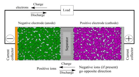
Figure 1.
Detailed structure of the interior of an electrochemical cell of a lithium ion (Li-ion) battery.
ions move around inside the cell, and the electrons detached from the oxidation reaction travel through the external circuit as shown in Equation (1). These ions are converted to Li when the electrons are available and then stored in the electrodes as shown in Equation (2) [15].
The electrolyte allows the transport of lithium ions; hence, there must be electrochemical reactions on the surface that allow this ion to enter the electrolyte. Thus, in this interface, the opposite charge accumulates to form a double layer, which acts as a capacitor. On the other hand, thanks to the ability of carbon to insert lithium with a stable SEI, lithium ions do not change the structure crystalline network of the material that acts as a host. The most common material used as a negative electrode is LiC6, whereas carbon (in graphite form) is the material that stores lithium between its graphite layers [16,17,18].
Li-ion batteries are very widespread in the field of energy storage due to their good characteristics. These are used in pure battery electric vehicles (BEVs), plug-in electric vehicles (PHEVs), and hybrid electric vehicles (HEVs) as a total or partial replacement for gasoline to achieve modern transport more beneficial for the environment.
There are battery models, very simple computationally speaking, based on the calculation of the internal impedance in series with the open-circuit voltage (OCV). In turn, this internal impedance is modeled by a resistor in series with a circuit, consisting of another resistor and a parallel capacitor. The OCV value depends on SOC and the temperature. For the values of internal impedance, the values of voltage and current measured in the battery are used. However, these models do not take into account the electrochemical processes that take place inside the battery, which depend on both internal and external aspects. The electrochemical model, which takes into account the transport of charge inside the cell, the intercalation process that takes place in the solid phase of the interior of the electrode materials, and the phenomena of electrochemical kinetics, is very precisely adjusted to the real situation of the battery and predicts it with enormous accuracy [17].
In this case, the problem is the time it takes to computationally solve this model, making it an unusable model in real time. Therefore, other models were developed as they are capable of making the same predictions, but solving less complex equations and, thus, using less time. In this paper, some of the most significant ones are addressed, for example, the SPM, which converts a model of five equations in partial derivatives and an algebraic equation to a model of only one equation with partial derivatives and an algebraic equation [16,17].
2.1. Electrochemical Model
The main idea behind storing energy in an Li-ion cell is that the energy released when the lithium is placed in an insert area of the positive electrode is different from the energy released when it is placed in an insertion site of the negative electrode. In comparison, lithium has much higher energy when stored in the negative electrode. These released energies are related to the electrochemical potential; thus, the electrostatic potential can be expressed as a function of the amount of lithium stored in the electrode. This electrostatic potential is equivalent to the mentioned OCV of the electrode. Next, the equations that describe the behavior of an Li-ion battery are presented [19].
The input to the model is the current applied to cell , and the output is the potential difference between its electrodes, which is obtained from Equation (3).
where is the electrical potential in the solid electrode.
It can be seen in Figure 2 that and 0 refer to the respective positions of the variable throughout the cell. This complete electrochemical model consists of six state variables that include the electric potential in the solid electrode, the electric potential in the electrolyte, the ion concentration of the active material in the positive and negative electrodes, the Li-ion concentration in the electrolyte, the ionic current in the electrolyte, and the ionic molar flow [15].
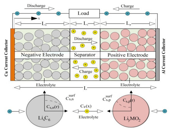
Figure 2.
One-dimensional schematic of the electrochemical model of an Li-ion cell.
As a result of combining Kirchhoff’s law with Ohm’s law relating and , the potential in solid electrodes results from
where, is the effective electronic conductivity of the complete electrode. As the electrode is porous, only a fraction of its volume contributes to its electronic conductivity. As boundary conditions of Equation (4), it could be established that, at the interface between the electrodes and the current collectors, there is zero ionic current , or that, at the interface between the electrodes and the separator, . The relationship between the potential of the electrolyte and the ionic current is given by
where is the average molar activity coefficient in the electrolyte and represents the deviations of the electrolyte solution compared to the expected ideal behavior; it is a function of the electrolyte concentration. Moreover, is the ionic conductivity of the electrolyte. The boundary conditions to obtain are established as , and, at the interfaces between the separator and both electrodes, the electrolyte potentials remain the same [20].
The concentration of Li-ion in solid particles is obtained from the diffusion of lithium in the solid phase. Since the model in the solid phase is associated with a spherical particle of radius and with spatial location that corresponds to that sphere, the transport of Li-ions responds to a diffusion gradient in the spatial domain as follows [20]:
where the initial and boundary conditions are given as
These boundaries imply that, on the surface of the particles, the ratio in which the ions leave the particle and access the electrolyte is given by the porous wall molar flow , and this ratio is zero when reaching the center of the particle. This can be seen in Figure 3, in the profiles that adopt the concentrations inside the anode and cathode spheres (flat profile in the area of ). The initial condition establishes the initial concentration profile of the particle, which does not need to be constant. Furthermore, this value is constant if the battery is initially at rest for a long time and the ions are “settled” in a uniformly constant state along the radius and position of the particle [20,21,22].
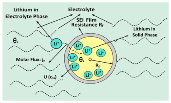
Figure 3.
Diagram of molar flux and associated transition of lithium from solid phase to electrolyte phase in the electrode domains.
It is important to note that the diffusion between adjacent particles is neglected, and no term of the type is considered in Equation (6), because it is insignificant given the high impedance of phase diffusion solid between particles. The concentration of Li-ion in the electrolyte changes due to a concentration gradient induced by a diffusion flow of ion and current . Therefore, it can be shown that
The first term in Equation (7) reflects the change in concentration due to diffusion, while the second term reflects the change due to the current and its gradient. Boundary conditions capture the fact that ion flux is zero at all times in current collectors. Since the flow is proportional to the concentration gradient in the collectors, it can be written as shown in Equation (8).
Since there are three spatial domains, four additional boundary conditions are required at the spacer electrode interfaces. These conditions are obtained from the continuity of flow as shown in Equations (9) and (10), while the concentration of the electrolyte at the interfaces is shown in Equations (11) and (12).
In each of the three main parts of the cell (both electrodes and the separator), the porous wall molar flow is related to the current divergence; thus,
where is the specific interfacial area, , and is the volume fraction of the solid electrode material in the porous electrode. For the boundary conditions, we have in the current collectors, and , while maintaining the continuity of the current must be established for both sides of the separator. The molar flow depends on the concentration of lithium in the solid and the concentration of lithium in the electrolyte [23].
For this, the Butler–Volmer equation describes the relationship between it and the over potential, given by Equation (14) [23].
where the over potential of the solid-phase intercalation reaction determines the rate of the reaction, which is given by
while and are the transfer coefficients and is the exchange current density.
With all this, it can be affirmed that the electrochemical model of a battery is a system composed of an algebraic equation (Equation (14)) and five nonlinear equations in partial derivatives, i.e., Equations (4), (6), (7) and (13), in addition to the output that is obtained from Equation (3).
As already mentioned, the concentration in the solid particle depends on the radius of the sphere based on which the electrode material is modeled. This value also depends on the position that this particle takes inside the electrode. The solid inside an electrode provides a very large area of contact with the electrolyte as shown in Figure 3. Therefore, a particle that is in an area closer to the collector does not have the same concentration as another that is closer next to the separator, for example. For the reaction corresponding to the solid-phase lithium intercalation, the over potential represents the deviation between the difference of equilibrium thermodynamic potential in the existing surface concentration and the difference of potential for a charged species that would cross when passing the SEI, between the solid electrode and the electrolyte [23,24].
The electric potential in the solid particle is called and the electric potential in the electrolyte is called . On the other hand, the difference in thermodynamic potential in the existing surface concentration is given by , that is, by the open-circuit potential of the intercalation reaction. The surface concentration of lithium in the solid particle is referred to as . The additional potential fall in the SEI is modeled by the resistance of the RSEI molecule [24,25].
2.2. Single-Particle Model (SPM)
The SPM was first proposed in Reference [15]. The model is based on the approximation that the current applied to the battery is small and that the conductivity of the electrolyte is large [16]. In this model, the properties of the electrolyte are ignored, which makes the transport phenomena simpler. However, the effects of thermal conditions on the performance of the Li-ion battery are considered. Its main drawback is that it must be adjusted according to the properties of the electrolyte for thick electrodes and at high discharge rates [26].
More specifically, as shown in Figure 4, each electrode in the SPM is modeled by a single spherical particle in which interleaving phenomena develop. Furthermore, variations in concentration in the electrolyte () and variations in potential are ignored.
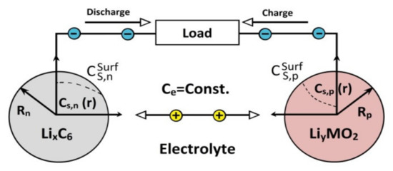
Figure 4.
Schematic of the single-particle model (SPM) of an Li-ion cell.
With these approximations, it can be achieved that the state variables, such as the concentration of Li-ion in solid particles , do not depend on the position of the part. Since each electrode is represented by only one particle, the dependency on the X-axis is eliminated, taking .
Using the approaches described above, the algebraic Equation (14) and the five partial derivative equations (PDEs) of the electrochemical model are simplified into two PDEs, one for each electrode (Equation (18)) and the algebraic Equation (22) [26].
The molar flux for each electrode is given by the following equation:
The concentration of Li-ion in the solid part of the electrode is
where the initial condition and the boundary conditions are
The potential difference between the cell terminals is
where, the electrode potentials and are given by
In this equation, the term by definition, which can be obtained from the solution of Equation (18).
The equations for the OCV of both electrodes depend on the stoichiometric coefficient of the electrode [17], whose value is . The parameter is substituted in the variable of Equation (24), and is replaced by in Equation (25) [27].
As a conclusion, it can be noted that the SPM responds with the battery voltage of Equation (22) from the current applied to the cell. Using Equation (23) on each electrode, it is necessary to apply Equations (24) and (25) to solve Equation (18), where the necessary variables are obtained to solve the model. In both Figure 3 and Figure 4, the concentration on the surface is referred to with the name or , depending on the electrode being used. However, in the equations, it is referred to with the name in the electrochemical model and in the single-particle model (SPM) [28].
2.3. Three-Parameter Model (TPM)
The three-parameter model (TPM) was presented in Reference [16] and developed in Reference [18]. This model serves to solve the equation of the diffusion of lithium in the solid particle, and it can be complemented by the remaining algebraic equations of the SPM. When the model uses volume-averaged equations and a parabolic profile approximation for the solid-phase concentration, the solid-phase partial differential equation reduces to two ordinary differential equations [24,25,26,27,28].
A more precise approximation was developed assuming that the solid-state concentration inside the spherical particle can be expressed as a polynomial in the spatial direction [19]. This develops approximate solutions for solid-phase diffusion based on approximations of polynomial profiles for constant porous wall molar flow at the surface of the particle. However, these models cannot be used directly for battery modeling because the porous wall flux on the surface of the particle changes as a function of time or as a function of distance through the porous electrode.
The model to be studied was developed for micro scalar diffusion with porous wall flow that depends on time, reducing computational simulation time, but without compromising precision. The differential equation for the diffusion equation on a spherical electrode particle is given by
If the diffusion constant of said material does not depend on the radius of the spherical particle, it can leave the partial derivative, where
This is the same equation that was analyzed in the previous models (Equations (6) and (18)), and whose initial condition and boundary conditions are also the same. A solution is proposed in parameters of the following type:
Substituting Equation (28) into Equation (27), we get
In this way, the boundary condition is maintained for ; however, if , it is converted from Equation (22) to Equation (30).
For battery modeling, there is great interest in knowing the averaged concentration in volume to obtain the SOC, the surface concentration for the electrochemical behavior, and the flow of the concentration averaged in the volume that physically defines the average change in the concentration with respect to the position of the system. In this way, the constants , , and are solved in terms of these last three variables. The averaged concentration in volume is given by
From Equation (28), becomes as follows:
The concentration at the surface is obtained by evaluating at the surface .
The flow of the average concentration in the volume is given by
Equation (35) is the updated version of Equation (34), similar to Equation (32).
Finally, the functions , and are written as follows:
Substituting Equations (36)–(38) in the equation proposed as a solution, the concentration in Equation (28) becomes as shown in Equation (39).
Applying volume averaging to the initial differential Equation (27) gives
Substituting Equation (39) into Equation (40), the equation of the averaged concentration becomes
where the initial condition for a new cell that is fully loaded would be . Thus, the same process can be done, but with the equation of the averaged flow.
Substituting from Equation (39) into Equation (42), the flow equation of the averaged concentration becomes
where the initial condition for a new cell that is fully loaded would be . The concentration of lithium on the surface of the particles is obtained by substituting Equations (37) and (38) into Equation (30) to give
In summary, it can be said that the TPM is made up of Equations (41), (43) and (44), which allows solving the concentration of lithium on the surface of the particles that make up each electrode.
3. Results and Discussion
In this section, the results of the previously introduced sections are presented and analyzed, where the calculations are carried out using the two models presented in Section 2. Additionally, a complete comparison between the two models is done, and all required data for the parameters are summarized in Table 1 and Table 2.

Table 1.
Cell model parameters [29].
Table 2.
Cell model parameters [29].
Starting from an electrochemical cell, a simulation of the complete discharge of this cell could be carried out. This means that the cell was initially owned at 100% SOC and it was intended to bring it up to 0% SOC using both models. When 0% of the SOC was reached, the current would be cut to avoid overloads in the cell and the responses of both models could be observed.
Firstly, the graphs of different interesting variables that could be obtained from the SPM were analyzed. It is necessary to remember that the SPM basically establishes that each electrode can be modeled by a single spherical particle that allows obtaining a matrix, whose sizes are those of the time and frequency vectors. Therefore, when the concentration of lithium in the particle is represented, the increases and decreases in the concentrations of both electrodes over time and frequency can be visualized. However, since many points are placed in the time vector to obtain more precision in the cell output voltage curve, this vector is reduced in order to clearly observe the change in the surface of the matrix.
The concentration in the positive electrode of Li-ion cell increased as it discharged, where, during that process, a reduction reaction occurred in the positive electrode which absorbed electrons that were released in the oxidation process of the negative electrode. Those electrons circulated through the circuit outside the cell and joined with the Li+ ions that reached the electrolyte inside the cell, leading to an increase in concentration. For the same reason, the concentration decreased with time at the negative electrode. It can be seen in Figure 5 and Figure 6 how the radius vector gradually deformed to the concentration closest to the outside of the sphere . It reached its maximum and minimum value, depending on whether it was the positive or negative electrode, respectively. After that maximum (or minimum) peak at which the cell reached its full discharge, the concentration was balanced across the sphere as the current became 0 and the Li-ions were reorganized.
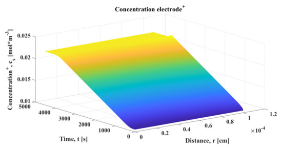
Figure 5.
Concentration (Li+) in the positive electrode of the cell (single-particle model (SPM)).
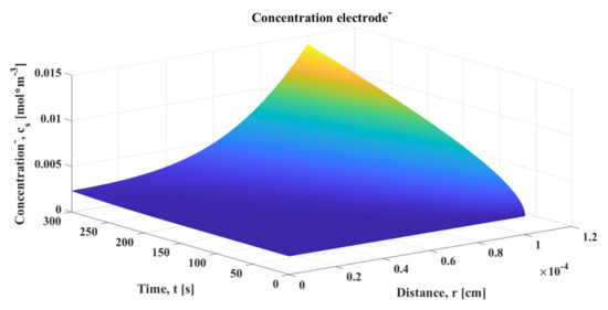
Figure 6.
Concentration (Li+) in the negative electrode of the cell (SPM).
In Figure 7, it can be clearly noted that the concentration profile was more abrupt on the outside of the sphere. Figure 8 introduces the profile for the negative electrode; however, the evolution of the profile is indicated. The representations belong to one discharge (termed 1C), and, despite the fact that a maximum (minimum in the case of the negative electrode) of concentration in the radius was observed, as the discharge rate increased, so did that extreme.
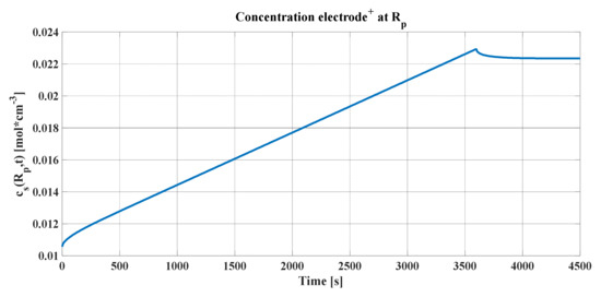
Figure 7.
Concentration (Li+) on the surface of the positive electrode (SPM).
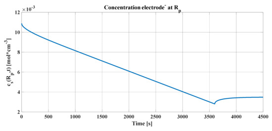
Figure 8.
Concentration (Li+) on the surface of the negative electrode (SPM).
The peak produced in the concentration profiles can be justified, as explained previously, assuming that the electrochemical cell must be cut when the average concentration in the radius of the particle reaches the maximum, as seen in Figure 9a,b. It represents the concentrations averaged in volume (blue line) for each of the graphs, the maximum and minimum of which must be maintained so that the stoichiometric coefficient of the concentration of lithium does not leave its variation ranges. In addition, the concentrations in the radius of the particle and in the center were added (green and black lines, respectively).
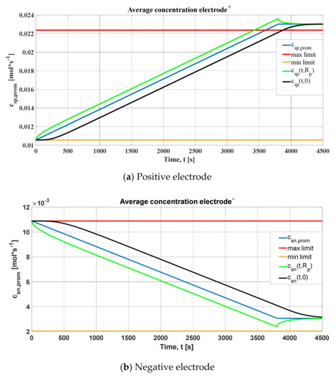
Figure 9.
Average (Li+) concentrations in both electrodes of the cell (SPM): (a) positive electrode; (b) negative electrode.
An important detail of these graphs is that, after the discharge current is cut, the concentration profiles in the radius and in the center tend toward the same value. By definition, Li-ions are reorganized in the electrode particle. Consequently, it can be concluded that the output voltage of the lithium cell for this simulation has the form shown in Figure 10. In this discharge, it can be noted that the range of variation of the potential difference of this cell has typical values of voltage. Furthermore, when the current is 0, the voltage curve responds temporarily to the reorganization of the lithium concentration in both spheres of the electrodes. From this transient response, the parameters of other types of non-electrochemical models for the batteries are obtained.
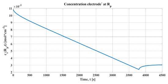
Figure 10.
Electrochemical cell concentration (SPM).
At this point, it is necessary to explain what happened using the TPM for the same conditions. Remember that, in this model, there is no longer any dependence on the radius of the particle of each electrode, that is, each electrode is modeled as if it were a point in space, whose concentration only changes with time. There was only an average concentration, whose shape with respect to time was as shown in Figure 11, which is very similar to that obtained in Figure 9. It can be noted in this figure that the concentration in the positive electrode increased, while it decreased in the negative one, as expected in a discharge. Furthermore, the concentration remained constant at the initial value when the current was cut off, after reaching the peak of the minimum voltage. However, the concentrations would not remain constant at the value they maintained, since the cut that was made affected the current, which became 0.
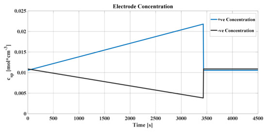
Figure 11.
Concentration in both electrodes of the cell (TPM).
Based on Figure 12, showing the cell output voltage for this model, the same thing happened as for the concentration. It suffered a sudden cut; however, in this case, there was no transient stabilization after the power cut, as was the case in SPM. Therefore, the voltage drastically returned to its value for discharge at a current of 0 A.
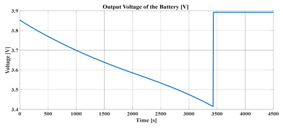
Figure 12.
Cell output voltage (TPM).
For a comparison between both models, both stress graphs are presented in Figure 13. The comparison of the discharge with cut-off is presented in Figure 13a, while the SPM discharge voltage and the discharge voltage of the TPM were practically identical, following an almost superimposed discharge curve, as shown in Figure 13b. The cells in both models were allowed to discharge for up to 3780 s to check if the coincidence of both voltages was maintained over time in case the discharge current was not cut off. It can be noted in the figure how the coincidence for a discharge rate of 1C was very precise.
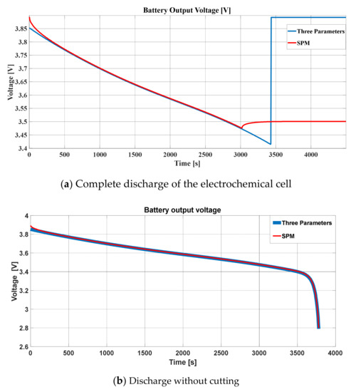
Figure 13.
Comparison of the output voltages of both models after a discharge at 1C: (a) complete discharge of the electrochemical cell; (b) discharge without cutting.
To consider the degradation of the battery based on the SPM, the battery output voltage should be studied for many cycles of discharging, whereby Figure 14 shows the voltage performance of the battery in such a situation. It can be noted that, as the discharging times increased, the output voltage decreased with the time. Figure 14 illustrates the influence of discharging time on the SOC.
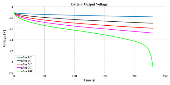
Figure 14.
The battery output voltage vs. the discharging rates based on the SPM.
Moreover, the charging performance was impacted by the number of discharging times; this is described in Figure 15, with a range of one to 10 discharging cycles based on the color legend of Figure 14. Furthermore, the battery output voltage had a weakness due to a high number of discharging times even when charged. Thus, discharging should be controlled to avoid the battery degrading; based on many studies, if the SOC becomes lower than 25%, the battery will degrade.
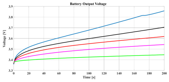
Figure 15.
The charging performance of the battery with respect to the discharging time based on the SPM.
The same scenario was easily repeated using the TPM in Figure 16, which, based on the same color notification of Figure 14, describes the battery output voltage. Many lines describe the voltage, where each line represents the battery voltage according to a certain number of discharging times of the battery.
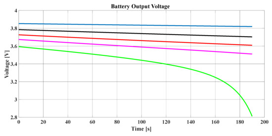
Figure 16.
The battery voltage based on the TPM.
To confirm the degradation of the battery, its voltage performance after charging was studied as shown in Figure 17 for a different number of battery discharging times.
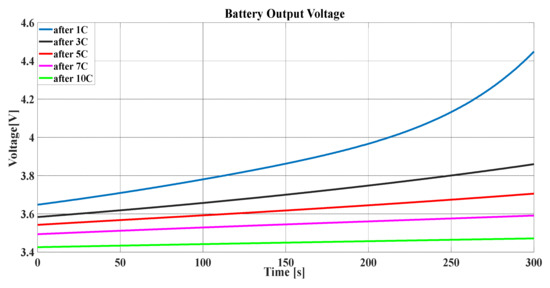
Figure 17.
The different voltage performances after charging based on the TPM.
Throughout the simulation codes, all the parameters obtained from Table 1 that appeared in the model equations were applied; however, for the value of the constant of speed of reaction—also called constant of the rate of reaction —there is no precise type of bibliography. In Reference [4] and in other references, there is a parameter that depends on the temperature and the charge transfer coefficient . Furthermore, the relationship between the constant in Reference [4] and that obtained from Reference [16] as , where is the Faraday constant. Despite this, the reaction rate constant plays an important role in the formation of SEI films in the anode. In Reference [21], a table with reaction rate constants for different electrochemical cells is shown, showing the dependence of this value on temperature. The values in this table range from s to s; however, it should be mentioned that, in the majority of articles searched, this parameter varies between s and s. It was also observed in their experimental results that this value increases with increasing temperature. Here, the dependency of the simulation results with different values of the reaction rate constant was evaluated in the SPM model created, as shown in Figure 18. Comparing the values tested in this figure with those in the range of Reference [21], it should be kept in mind that the Faraday constant intervenes in the conversion of the values, due to the variation of from 1 to .
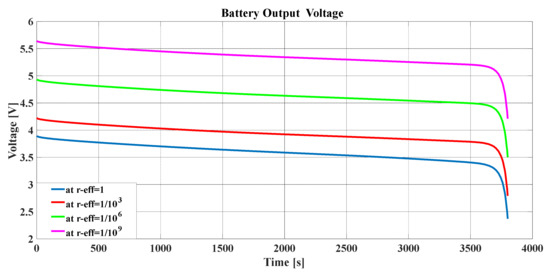
Figure 18.
The battery discharging voltage at different values of .
MATLAB codes were developed in this work to calculate the capacity of the battery and the discharging (C) rate for the simulation being carried out and the SOC of the battery at each point of the simulation. The SOC of a battery can be related to the total amount of lithium found in each of the electrodes. Similarly, by dividing the total amount of lithium in any electrode by the total volume of the solid active material in which it resides, the SOC can be related to the average concentration of lithium in the negative or positive electrodes, where the average is calculated over the entire electrode [4]. When the cell is fully charged, the amount of lithium on the negative electrode is at its maximum allowable level and the amount of lithium on the positive electrode is at its minimum allowable level. In stoichiometric terms, and, analogously, .
Similarly, when the cell is completely discharged, the amount of lithium on the negative electrode is at its minimum allowed level, and the amount of lithium on the positive electrode is at its maximum allowed level. That is to say, and . It can be deduced simply that, if, for example, the positive electrode is at its maximum level when the cell is discharged, then ; as a consequence, . The SOC varies linearly as does the stoichiometry at each electrode; therefore, in Figure 19, the way in which the voltage increases as the battery is charged can be visualized. If the SOC is plotted against time, an ascending or descending straight line would be observed depending on the load or discharge, respectively. In this case, the slope would depend on the rate of charge or discharge. Hence, SOC is equal to the difference of and , and this difference is divided by the difference of and . The resultant ratio is equal to the ratio of . Finally, Figure 19 and Figure 20 show the SOC based on the two discussed methods (SPM and TPM, respectively). Additionally, it can be noted that the SOC is severely influenced by the number of discharging times.
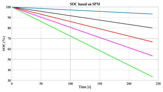
Figure 19.
The state of charge (SOC) of the battery with respect to the discharging times based on the SPM.
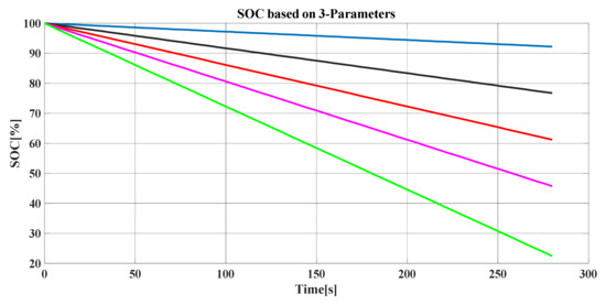
Figure 20.
The different SOCs of the battery based on the TPM.
The hybrid pulse power characterization (HPPC) [23] is intended to determine the dynamic power capacity over the usable voltage and load range of a device using a test profile that incorporates regeneration and discharge pulses. The normal test protocol uses constant current (not constant power) at levels derived from the manufacturer’s maximum nominal discharge current. The characterization profile is shown in Table 3 and Figure 21.
Table 3.
The hybrid pulse power characterization (HPPC) test profile [23].
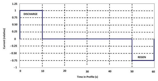
Figure 21.
Profile of the HPPC test.
The currents are indicated relatively, according to the C rate, in order for the test to be universal. It should also be mentioned positive current values are used for discharges and negative values are used for charges. The test is made up of unique repetitions of this profile, separated by constant current discharge segments until reaching 10% depth of discharge (DOD), followed by a one-hour rest period to allow the cell to return to thermal and electrochemical equilibrium before applying the following profile. The test starts with a fully charged device after one hour of rest and ends after completing the final profile at 90% DOD, the cell discharge at a rate at 100% DOD, and a final break of one hour. The voltages during each rest period are recorded to establish the behavior of the cell’s OCV. The sequence of rest periods, pulse profiles, and discharge segments for are illustrated in Figure 22. This figure also illustrates a download that must be run just before each HPPC test. The complete test was performed with nine sequences of the profile in Figure 21 in the same way as the two sequences of the HPPC profile in Figure 23.
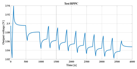
Figure 22.
Output voltage of the battery when subjected to the HPPC test.
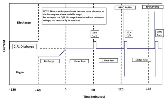
Figure 23.
HPPC test sequences [23].
In Reference [30], the same test was carried out with a real battery, specifically an LiMn2O4 battery (PL60110190) with a nominal capacity of 50 Ah and 185 Wh. The complete pack consisted of 16 cells connected in series, where each one was equipped with an active balancing module to ensure that the discharge voltage and capacity remained constant during operation. Figure 24 shows the simulation and the carried out test results. The HPPC test was carried out for the 50 Ah battery, and it is easy to note the similarity between the test and simulation results.
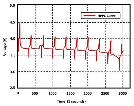
Figure 24.
The output voltage of the battery used in Reference [24] when subjected to the HPPC test.
The change in the time scales for both figures and in some periods of rest was due to the fact that, in the SPM, the input of the discharge current vector, which is shown in Figure 25, could not be entered in the same way as in the test controlled on a real battery.
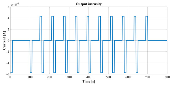
Figure 25.
Vector of the current applied to the electrochemical cell.
The remaining representations obtained from the HPPC test are shown in the figures below, where Figure 26 and Figure 27 show the concentrations of the positive and the negative electrodes, respectively. Figure 9a,b is repeated for the concentrations of the positive and negative electrodes based on the HPPC test procedure. Figure 28a shows the concentration of the positive electrode, while Figure 28b represents the negative electrode concentration; the shown fluctuations are due to the sudden changes in the HPPC procedure.
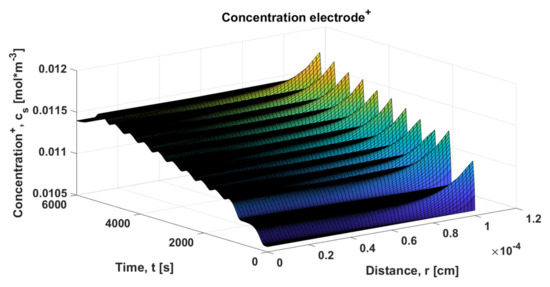
Figure 26.
Li+ concentration on the positive electrode.
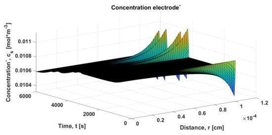
Figure 27.
Li+ concentration on the negative electrode.
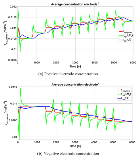
Figure 28.
Averaged concentrations in the sphere volume based on the HPPC procedure: (a) positive electrode concentration; (b) negative electrode concentration.
4. Conclusions
The internal operation of an Li-ion battery was studied in depth with different models, while explanations were given for the electrochemical phenomena that take place inside. These models were implemented in Matlab to study certain phenomena in the same way as if we were working with real electrochemical cells. Three very important models—the electrochemical model, the SPM, and the TPM—were explained in detail, each with their corresponding assumptions. The implementations were carried out for the SPM and the TPM, and the results of these models were presented and compared. As an outstanding conclusion, it can be stated based on the obtained representations that the two models had great similarities (more in charge than in discharge) in their tension and concentration curves. There was only a slight difference between the models at a high C-rate. Another significant detail is that the models included a method of cutting the current in charge and discharge in order to protect the battery based on the maximum stoichiometric ranges of the concentration of lithium in its electrodes. It can also be concluded that the parameter had a direct influence on the discharge voltage of the electrochemical cell and, since this value depended on the temperature, its variation directly affected the cell. The previous literature indicated this parameter without precisely clarifying its dependence on other parameters; however, in this work, the discharge voltage was studied at different values of .
Author Contributions
Conceptualization, M.A.-G.; data curation, M.A.-G. and N.S.H.; formal analysis, M.A.-G. and S.A.H.; methodology, M.A.-G. and N.S.H.; resources, N.S.H. and S.A.H.; software, N.S.H.; supervision, M.A.-G.; validation, S.A.H.; Visualization, M.A.-G. and N.S.H.; Writing—original draft, M.A.-G. and N.S.H.; Writing—review and editing, M.A.-G., S.A.H. and N.S.H. All authors together organized and refined the manuscript in the present form. All authors have read and agreed to the published version of the manuscript.
Funding
This research received no external funding.
Conflicts of Interest
The authors declare no conflict of interest.
References
- Wei, X.; Yimin, M.; Feng, Z. Lithium-ion Battery Modeling and State of Charge Estimation. Int. Ferroelectr. 2019, 200, 59–72. [Google Scholar] [CrossRef]
- Pozzi, A.; Ciaramella, G.; Volkwein, S.; Raimondo, D.M. Optimal design of experiments for a lithium-ion cell: Parameters identification of a single particle model with electrolyte dynamics. Ind. Eng. Chem. Res. 2019, 58, 1286–1299. [Google Scholar] [CrossRef]
- Hinz, H. Comparison of Lithium-Ion Battery Models for Simulating Storage Systems in Distributed Power Generation. Inventions 2019, 4, 41. [Google Scholar] [CrossRef]
- Wang, A.; Kadam, S.; Li, H.; Shi, S.; Qi, Y. Review on modeling of the anode solid electrolyte interphase (SEI) for lithium-ion batteries. NPJ Comput. Mater. 2018, 15, 1–27. [Google Scholar] [CrossRef]
- Meng, J.; Luo, G.; Ricco, M.; Swierczynski, M.; Stroe, D.I.; Teodorescu, R. Overview of Lithium-Ion Battery Modeling Methods for State-of-Charge Estimation in Electrical Vehicles. Appl. Sci. 2018, 8, 659. [Google Scholar] [CrossRef]
- Chen, Y.; Huo, W.; Lin, M.; Zhao, L. Simulation of electrochemical behavior in Lithium ion battery during discharge process. PLoS ONE 2018, 13, 1–16. [Google Scholar] [CrossRef]
- Berrueta, A.; Urtasun, A.; Ursúa, A.; Sanchis, P. A comprehensive model for lithium-ion batteries: From the physical principles to an electrical model. Energy 2018, 144, 286–300. [Google Scholar] [CrossRef]
- Barcellona, S.; Piegari, L. Lithium Ion Battery Models and Parameter Identification Techniques. Energies 2017, 10, 2007. [Google Scholar] [CrossRef]
- Saidani, F.; Hutter, F.X.; Scurtu, R.G.; Braunwarth, W.; Burghartz, J.N. Lithium-ion battery models: A comparative study and a model-based power line communication. Adv. Radio Sci. 2017, 15, 83–91. [Google Scholar] [CrossRef]
- Abada, S.; Marlair, G.; Lecocq, A.; Petit, M.; Sauvant-Moynot, V.; Huet, F. Safety focused modeling of lithium-ion batteries: A review. J. Power Sources 2016, 306, 178–192. [Google Scholar] [CrossRef]
- Subramanian, V.R.; Boovaragavan, V.; Ramadesigan, V.; Arabandi, M. Mathematical Model Reformulation for Lithium-Ion Battery Simulations: Galvanostatic Boundary Conditions. J. Electrochem. Soc. 2009, 156, 260–271. [Google Scholar] [CrossRef]
- Subramanian, V.R.; Boovaragavan, V.; Diwakar, V.D. Toward Real-Time Simulation of Physics Based Lithium-Ion Battery Models. Electrochem. Solid State Lett. 2007, 10, 255–260. [Google Scholar] [CrossRef]
- Du Pasquier, A.; Plitz, I.; Menocal, S.; Amatucci, G. A comparative study of Liion battery, super capacitor and no aqueous asymmetric hybrid devices for automotive applications. J. Power Sources 2003, 115, 171–178. [Google Scholar] [CrossRef]
- Jokar, A.; Rajabloo, B.; Désilets, M.; Lacroix, M. Review of simplified Pseudo-two Dimensional models of lithium-ion batteries. J. Power Sources 2016, 327, 44–55. [Google Scholar] [CrossRef]
- Chae, S.; Ko, M.; Kim, K.; Ahn, K.; Cho, J. Confronting Issues of the Practical Implementation of Si Anode in High-Energy Lithium-Ion Batteries. Joule 2017, 1, 47–60. [Google Scholar] [CrossRef]
- Plett, G.L. Battery Management Systems, Volume 1: Battery Modeling; Artech House: London, UK, 2015. [Google Scholar]
- Faulkner, L.R. Understanding electrochemistry: Some distinctive concepts. J. Chem. Educ. 1983, 60, 262–271. [Google Scholar] [CrossRef]
- Broussely, M.; Biensan, P.; Simon, B. Lithium insertion into host materials: The key to success for Li ion batteries. Electrochim. Acta 1999, 45, 3–22. [Google Scholar] [CrossRef]
- Nitta, N.; Wu, F.; Lee, J.T.; Yushin, G. Li-Ion battery materials: Present and future. Mater. Today 2015, 18, 252–264. [Google Scholar] [CrossRef]
- Kaiser, R. Optimized battery-management system to improve storage lifetime in renewable energy systems. J. Power Sources 2007, 168, 58–65. [Google Scholar] [CrossRef]
- Chaturvedi, N.A.; Reinhardt, K.; Christensen, J.; Ahmed, J.; Kojic, A. Modeling, Estimation, and Control Challenges for Lithium-Ion Batteries. In Proceedings of the 2010 American Control Conference, Baltimore, MD, USA, 30 June–2 July 2010; pp. 1997–2002. [Google Scholar]
- Tran, N.T.; Vilathgamuwa, M.; Farrell, T. Matlab Simulation of Lithium Ion Cell Using Electrochemical Single Particle Model. In Proceedings of the 2nd Annual Southern Power Electronics Conference, Auckland, New Zealand, 5–8 December 2016; pp. 1–6. [Google Scholar]
- Smith, K.; Wang, C.Y. Solid-state diffusion limitations on pulse operation of a lithium ion cell for hybrid electric vehicles. J. Power Sources 2006, 161, 628–639. [Google Scholar] [CrossRef]
- Subramanian, V.R.; Diwakar, V.D.; Tapriyal, D. Efficient Macro-Micro Scale Coupled Modeling of Batteries. J. Electrochem. Soc. 2005, 152, 2002–2008. [Google Scholar] [CrossRef]
- Subramanian, V.R.; Ritter, J.A.; White, R.E. Approximate Solutions for Galvanostatic Discharge of Spherical Particles I. Constant Diffusion Coefficient. J. Electrochem. Soc. 2001, 148, 444–452. [Google Scholar] [CrossRef]
- Tanim, T.R.; Rahn, C.D. Aging formula for lithium ion batteries with solid electrolyte interphase layer growth. J. Power Sources 2015, 294, 239–247. [Google Scholar] [CrossRef]
- Ramesh, S.; Ratnam, K.V.; Krishnamurthy, B. An Empirical Rate Constant Based Model to Study Capacity Fading in Lithium Ion Batteries. Int. J. Electrochem. 2015, 162, 545–552. [Google Scholar] [CrossRef]
- Liu, D.; Cao, G. Engineering nanostructured electrodes and fabrication of film electrodes for efficient lithium ion intercalation. Energy Environ. Sci. 2010, 3, 1218. [Google Scholar] [CrossRef]
- Environmental Idaho National Engineering and Laboratory. Freedom CAR Battery Test Manual for Power-Assist Hybrid Electric Vehicles, Doe/Id-11069; Environmental Idaho National Engineering and Laboratory: Idaho Falls, ID, USA, 2003. Available online: https://avt.inl.gov/sites/default/files/pdf/battery/freedomcar_manual_04_15_03.pdf (accessed on 6 July 2020).
- Li, D.; Ouyang, J.; Li, H.; Wan, J. State of charge estimation for LiMn2O4power battery based on strong tracking sigma point Kalman filter. J. Power Sources 2015, 279, 439–449. [Google Scholar] [CrossRef]


© 2020 by the authors. Licensee MDPI, Basel, Switzerland. This article is an open access article distributed under the terms and conditions of the Creative Commons Attribution (CC BY) license (http://creativecommons.org/licenses/by/4.0/).