Article

Generalized Distribution of Relaxation Times Analysis for the Characterization of Impedance Spectra

1
Chair of Electrical Energy Systems, University of Bayreuth, Universitätsstraße 30, 95447 Bayreuth, Germany
2
Bayerisches Zentrum für Batterietechnik (BayBatt), Bayreuth, Universitätsstraße 30, 95447 Bayreuth, Germany
Batteries 2019, 5(3), 53; https://doi.org/10.3390/batteries5030053
Submission received: 15 May 2019 / Revised: 10 June 2019 / Accepted: 13 June 2019 / Published: 4 July 2019

Abstract

:
Impedance spectroscopy is a universal nondestructive tool for the analysis of the polarization behavior of electrochemical systems in frequency domain. As an extension and enhancement of the standard impedance spectroscopy, the distribution of relaxation times (DRT) analysis was established, where the spectra are transferred from frequency into time domain. The DRT helps to analyze complex impedance spectra by identifying the number of polarization processes involved without prior assumptions and by separating and quantifying their single polarization contributions. The DRT analysis, as introduced in literature, claims to be a model-free approach for the characterization of resistive-capacitive systems. However, a data preprocessing step based on impedance models is often required to exclude non-resistive-capacitive components off the measured impedance spectra. The generalized distribution of relaxation times (GDRT) analysis presented in this work is dedicated to complex superposed impedance spectra that include ohmic, inductive, capacitive, resistive-capacitive, and resistive-inductive effects. The simplified work flow without preprocessing steps leads to a reliable and reproducible DRT analysis that fulfills the assumption of being model-free. The GDRT is applicable for the analysis of electrochemical, electrical, and even for non-electrical systems. Results are shown for a lithium-ion battery, a vanadium redox flow battery, and for a double-layer capacitor.

1. Introduction

1.1. Generalized Impedance Spectroscopy

As stated above, impedance spectroscopy is a universal nondestructive tool for the analysis of the polarization behavior of electrochemical systems. In general, impedance corresponds to the transfer function of current and voltage in frequency domain
Z ( j ω ) = U ( j ω ) I ( j ω ) = u ^ ( ω ) sin ( ω t ) i ^ ( ω ) sin ( ω t + φ ( ω ) ) = | Z ( j ω ) | e j ω φ
The input or excitation signal could be current (galvanostatic mode) or voltage (potentiostatic mode). Electrochemical impedance spectroscopy (EIS) was applied to a variety of electrochemical systems covering, e.g., sensors [1], fuel cells [2,3], and batteries [4,5,6,7,8], as well as for material characterization that looks at transport and charge transfer processes, interface phenomena, conductivity, and diffusion [9,10,11,12]. Furthermore, impedance spectroscopy using current and voltage as excitation and system response is applied to photovoltaic cells [13,14] and under the label of bioelectrical impedance analysis (BIA) for clinical studies, tissue characterization [15], and for meat quality control [16,17].
Impedance spectroscopy is, in a generalized manner, applicable to the input-output behavior of systems in any physical domain. Therefore, the excitation of a system and its response [18] can be described by conjugated variables or, in analogy to the standard impedance definition, by the generalized voltage as intensive variable or across variable, and by the generalized current as extensive variable or through variable. Hence, the system’s input-output behavior or its transfer function is regarded as its generalized impedance. The applicability of this concept to a variety of physical domains is shown in Table 1. Examples of non-electric variables, where this concept was already used are, e.g., the pressure and voltage for an electrochemical pressure impedance spectroscopy [19,20], temperature and heat for an electrothermal spectroscopy [21,22], and the light intensity [23] for the analysis of photovoltaic systems.

1.2. Distribution of Relaxation Times Analysis

Where impedance spectroscopy describes the polarization behavior as a complex, frequency dependent function Z ( j ω ) , the distribution of relaxation times analysis, looks at the same input-output behavior in time domain, i.e., taking the Fourier transform of the spectrum into the focus. The DRT method recently gained attention in the field of electrochemical power sources [24] due to its powerful ability to analyze major and minor polarization effects even when overlapping in frequency domain, as shown in Figure 1, and its, in-principal, model-free approach [25,26,27,28,29].
The DRT analysis is based on a predefined distribution of N τ time constants [ τ min τ k τ max ] . In general, the choice of the distribution of time constants is mathematically independent of the measured frequency points. In most cases, N τ is chosen as a multiple of the number of measured frequencies in the impedance spectrum N f : N τ = c N f , with c { 1 , 2 , 3 } to get smoother distribution functions [30]. Usually, the minimum and maximum time constants are set according to the corresponding maximum and minimum frequencies of the spectrum, i.e., τ min = ( 2 π   f max ) 1 and τ max = ( 2 π   f min ) 1 . Mathematically, this choice is not compulsory. A broadening of the distribution of time constants might be beneficial for the calculation of the DRT, as shown in the results later.
The fundamental element to describe a resistive-capacitive behavior is the RC element, a parallel circuit of an ohmic resistor, and a capacitor with its impedance Z C = ( j ω C ) 1 . Throughout this document, C is used as a variable for a capacitor with its capacitance in F = As   V 1 . If the capacity (in Ah) of a storage device is addressed, the variable C Ah is used. The impedance of the parallel RC circuit is
Z R C = R 1 + j ω τ R C
with the characteristic time constant τ R C = R C . A Voigt model, a series of N parallel RC circuits with individual time constants τ k = R k C k , k = 1 N τ , is used to identify the polarization contribution of every single RC element at the predefined time constant resulting in a distribution function [ h 1 h k h N τ ] , where each h k value corresponds to the resistance of the corresponding RC element. The impedance spectrum of the distribution of relaxation times is described by
Z DRT ( j ω ) = k = 1 N τ h k 1 + j ω τ k = R pol k = 1 N τ g k 1 + j ω τ k
with g k being the normalized distribution of relaxation times function and R pol the overall polarization. The distribution function h ( τ ) is used to discuss the absolute contribution of single processes, g ( τ ) is used to discuss their relative contribution to the overall polarization of the device under test (DUT).
To illustrate the transformation of an impedance spectrum into a distribution function of relaxation times, Figure 2a shows an example spectrum of a series connection of an ohmic resistance, an RC circuit, and a ZARC element. The ZARC element
Z ZARC = R 1 + ( j ω τ R C ) φ
is a generalized RC circuit with an additional exponent φ that presents a depressed semi-circle in the Nyquist plot and that is used to describe imperfect capacitors (cf. constant phase element) or inhomogeneities. Table 2 shows the model values chosen for the impedance simulation.
In the Nyquist plot in Figure 2a, both resistive-capacitive elements overlap and cannot be separated sharply, whereas in the DRT in Figure 2b, both contributions are clearly separated into two peaks.

1.3. Solving the Optimization Problem of DRT Using Regularization

To match the distribution function of relaxation times to a measured impedance spectrum, an optimization problem needs to be solved that minimizes the error between model prediction and measured data, e ( j ω ) = Z meas ( j ω ) Z DRT ( j ω ) , in a least squares sense. To incorporate all information available, both real and imaginary parts of the error, e Re = Re { Z meas } Re { Z DRT } and e Im = Im { Z meas } Im { Z DRT } , are used for the definition of the cost function that needs to be minimized for best fit. The cost function of the optimization problem needs to be a scalar and real-valued function. Therefore, the sum of squared errors of e Re and e Im is used with individual weighting factors m and n for the real and the imaginary part
J = l = 1 N f m   e Re , l 2 ( τ ) + l = 1 N f n   e Im , l 2 ( τ ) = A   x b 2
In the following, the weighting factors are set to be equal, m = n = 1 . The definition of the cost function corresponds to a linear optimization problem, a linear system of equations A   x = b with the unknown, wanted distribution function of the DRT
x = [ h 1 h k h N τ ] T ,
the given real and imaginary parts of the measured spectrum
b = [ Re { Z meas } Im { Z meas } ] ,
and the matrix that needs to be calculated for the different measured frequencies and predefined time constants
A = [ Re { 1 1 + j ω 1 τ 1 } Re { 1 1 + j ω 1 τ N τ } Re { 1 1 + j ω N f τ 1 } Re { 1 1 + j ω N f τ N τ } Im { 1 1 + j ω 1 τ 1 } Im { 1 1 + j ω 1 τ N τ } Im { 1 1 + j ω N f τ 1 } Im { 1 1 + j ω N f τ N τ } ] .
The optimization problem min x 0 + { J } requires a non-negativity constraint, x k 0     k , for the DRT to yield physically meaningful results.
Calculating the DRT, the challenge faced is that the optimization problem in general is ill-posed, i.e., to solve the optimization problem in a physically relevant way, we need to apply regularization. Otherwise solving the optimization problem yields a scattered numerical solution that cannot be interpreted physically. The method mostly used is Tikhonov regularization [31,32,33], where the optimization problem is basically slightly varied by forcing the polarization of neighboring time constants not to differ that much, resulting in a smooth distribution function. Mathematically, the cost function
J = A   x b 2 + Γ   x 2
is extended by the regularization term Γ = λ   I that is, in most cases, defined as a multiple of the identity matrix I with the regularization parameter λ , other options are discussed in [30].
To solve the optimization problem above, some groups use an algorithm published by Weese [32] that was specifically developed for solving optimization problems with regularization. In general, any algorithm solving least squares problems with non-negativity constraints can be applied, e.g., the Lawson-Hanson algorithm for non-negative least squares [34]. Alternative methods for the calculation of the distribution of relaxation times function and a comparison to the Tikhonov regularization can be found in [35]. The calculation of the DRT using a regularization method offers degrees of freedom (cf. Table 3) that need to be published to get reproducible results.
To examine the sensitivity of the DRT calculation toward the process parameters of optimization and regularization, we recently published an extensive study [30]. Therein, we present a selection of process parameters that yield reliable and reproducible DRT results, where single polarization contributions can be separated and quantified. The algorithm used is available at http://www.ec-idea.uni-bayreuth.de within a software package based on the Matlab Runtime Environment. The algorithm of the generalized DRT presented here will be also available in a future release.

1.4. Analyzing Distribution Functions by Peak Analysis

The separation and quantification of single polarization contributions can be reached by a peak analysis of the DRT function with a first assumption of Normal or Gauss distributions within the DRT. Characteristic values are: 1. position, expectation of the distribution function that equals the characteristic time constant τ c of the process 2. height h , at first glance, an indication of polarization contribution, but it has to be discussed in conjunction with 3. standard deviation σ or variance σ 2 , an indication of width, a measure of homogeneity in spatially distributed processes if peaks are washed out. If asymmetric distribution functions are encountered, the standard definition of the Gauss distribution can be extended by 4. skewness α that tilts the Gaussian slightly to one side.
The probability density function (PDF) of the extended Gauss distribution is described by
g peak ( τ ) = h   exp { ( ( τ τ c ) ( 1 + α sgn { τ τ c } ) ) 2 2   σ 2 }
The polarization contribution of a single peak at a characteristic time constant is equal to the area the Gaussian bell covers, hence the integral of the Gauss distribution or the cumulative distribution function (CDF)
R peak = R pol g peak ( τ )   d τ R pol k = 1 N g peak ( τ k )
A stringent discussion of DRT requires the separation of single processes by their specific characteristic time constants and their polarization contribution to the overall polarization of the device under test as well as a discussion of the shape of the single peaks, i.e., the variance and skewness, to learn about homogeneity.
The example DRT in Figure 2b shows two peaks of the two resistive-capacitive elements of the modelled impedance spectrum. The height of both is almost identical. Yet, the polarization contribution differs by almost a factor of 2, which becomes obvious when the area both peaks cover is regarded.

1.5. Discussion of Shortcomings of DRT

Per definition the DRT function describes the resistive-capacitive behavior of an impedance spectrum. It has been extended to pure ohmic, inductive, and capacitive behavior by adding a serial resistor, inductor, and capacitor to the final DRT model spectra:
Z DRT ( j ω ) = k = 1 N τ h k 1 + j ω τ k + Z R + Z C + Z L = k = 1 N τ h k 1 + j ω τ k + R Ω + 1 j ω C + j ω L
In the workflow of DRT analysis, this was achieved by introducing a two-step preprocessing of the measured impedance data before the actual DRT analysis: 1. Modeling the measured impedance spectra in frequency domain and identification of model parameters by least-squares fitting and 2. Subtraction of purely ohmic, inductive, and capacitive effects from the measured spectrum by
Z meas , DRT = Z meas R Ω Z L Z C
resulting in a putatively resistive-capacitive spectra required for the DRT analysis. The work flow is shown in Figure 3a.
Diffusion phenomena lead to a diverging impedance behavior for low frequencies where the limit value lim ω 0 Z ( j ω ) does not converge against the real axis. These effects have to be identified and subtracted from the measured spectra in the same manner as above:
Z meas , DRT = Z meas R Ω Z L Z C Z diff
The approach described can be criticized for two reasons. First, the model-based preprocessing of the measured impedance spectra violates the assumption of DRT being a model-free method for the characterization of impedance spectra. Second, the subtraction of ohmic, inductive, and capacitive effects does not help for more complex impedance spectra, including superposed resistive-inductive behavior.

2. Generalized Distribution of Relaxation Times Analysis

The discussion of standard DRT above underlines the need for a Generalized Distribution of Relaxation Times (GDRT) analysis that fulfills the assumption of being model-free and that comprises ohmic, inductive, capacitive, and resistive-capacitive, as well as resistive-inductive effects. If this can be achieved, the work flow of DRT analysis can be simplified since the preprocessing of measured impedance data is eliminated. Hence, the fundamental approach of GDRT is to incorporate all basic types of impedance behavior in the calculation of the DRT, i.e., the equation to calculate the GDRT needs to include an ohmic resistance (offset from origin to positive real parts), a capacitance (diverging behavior for low frequencies), an inductivity (diverging behavior for high frequencies), and resistive-capacitive behavior (converging semi-circles in fourth quadrant with positive real part and negative imaginary part), as well as resistive-inductive behavior (converging semi-circles in first quadrant with positive real and imaginary part). Corresponding to the RC element in Equation (2), the fundamental element to describe the resistive-inductive behavior of a system is a parallel circuit of an ohmic resistance R and an inductivity with its impedance Z L = j ω L that together yield the impedance of the RL element
Z R L = j ω   τ R L   R 1 + j ω τ R L
with the characteristic time constant τ R L = L R .
In the generalized DRT analysis, the calculation of Z DRT is extended. Besides the standard impedance of the distribution function for the resistive-capacitive behavior (Equation (3)), an additional impedance of a distribution function for the resistive-inductive behavior is calculated. The added distribution function also is an equivalent Voigt model, a series of N τ parallel RL circuits with individual time constants τ R L , k = L k R k
Z Σ R L ( j ω ) = k = 1 N τ j ω τ k   h R L , k 1 + j ω τ k
where the predefined time constants are the same as for the resistive-capacitive distribution function. Together with the impedances of the pure ohmic, capacitive, and inductive contributions the equation of the GDRT impedance results:
Z GDRT ( j ω ) = Z Σ R C ( j ω ) + Z Σ R L ( j ω ) + Z R + Z C ( j ω ) + Z L ( j ω ) = k = 1 N τ h R C , k 1 + j ω τ k + k = 1 N τ j ω τ k   h R L , k 1 + j ω τ k + R Ω + 1 j ω C + j ω L
Instead of preprocessing the measured impedance data for the DRT analysis, in the GDRT analysis, the full DRT model, as described in Equation (17), is used for characterizing the measured spectra. The GDRT analysis results in two distribution of relaxation times functions for the resistive-capacitive behavior and for the resistive-inductive behavior, as well as three parameters: The ohmic resistance R Ω , the capacitance C , and the inductance L . Likewise, to the standard DRT, both distribution functions need to be non-negative to be physically meaningful.
The identification of the two distribution functions and the three lumped parameters in the GDRT analysis follows the same pattern as above: The cost function is defined the same as in the standard DRT (cf. Equation (5)). Regularization is applied in the same way as stated in Equation (9). The cost function again yields a linear system of equations A   x = b with differing definitions of the matrix A and the vector b . The unknown, wanted vector of the GDRT
x = [ h R C , 1 h R C , N τ   , h R L , 1 h R L , N τ   , R ,   L ,   C ] T ,
now comprises the two distribution functions of the resistive-capacitive behavior and the resistive-inductive behavior, as well as the three lumped parameters R , L , and C . The system matrix A has to be extended accordingly.
Figure 3b shows the work flow of the generalized DRT. The distribution of relaxation times functions can be calculated immediately for measured impedance spectra that comprise ohmic, inductive, capacitive, and resistive-capacitive, as well as resistive-inductive effects without the need of data preprocessing, especially without the need of impedance modelling. In this sense, the generalized distribution of relaxation times analysis fulfills the assumption of being a model-free approach for the characterization of impedance spectra. In comparison to the state of the art DRT the work flow of the GDRT is shortened significantly. Many degrees of freedom in impedance modelling and reduction of measured spectra were taken out improving considerably the reliability and reproducibility of the DRT analysis.

3. Results of GDRT Analysis

In the following, the impedance spectra of three very different electrochemical systems are analyzed and discussed using the introduced GDRT method. For a better comparability, the regularization parameter was set to λ = 0.2 for all analyzed spectra. An extensive study of the sensitivity of the choice of λ on the resulting distribution function can be found in [30].

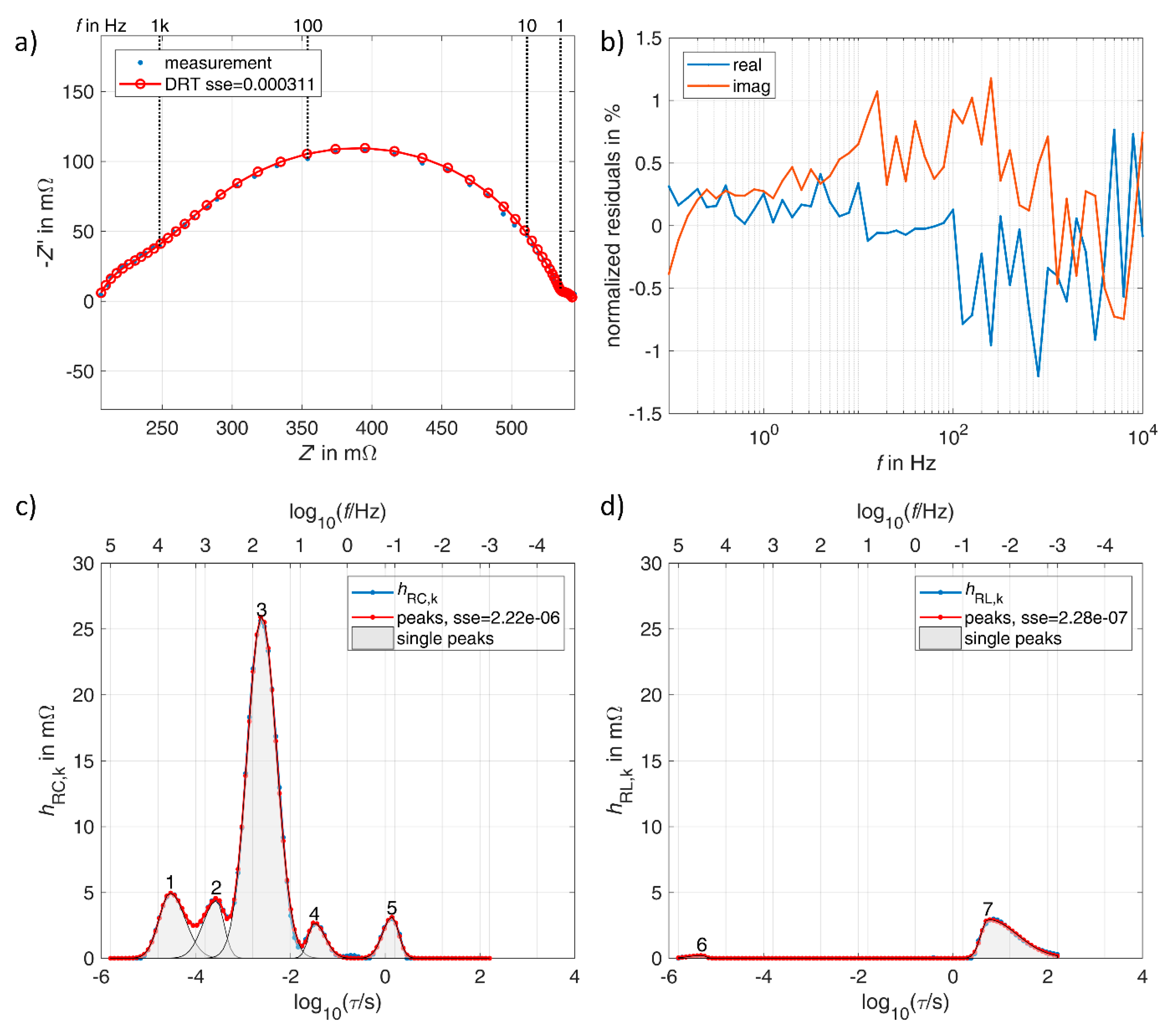
3.1. Lithium-Ion Battery

Lithium-ion batteries (LIB) present complex impedance spectra. The full cell comprises impedance contributions of the anode with its solid electrolyte interphase (SEI), the cathode, and the electrolyte, each with different polarization mechanisms: Conductivity, charge transfer, and double layer effects, as well as diffusion processes [36].
The system under study is a LIB of the producer A123 Systems with the cell chemistry LFP | graphite, the cell format 26650 and a nominal capacity of C Ah = 2.5   Ah . The impedance spectrum was measured with a minimum frequency of f min = 52   mHz , a maximum frequency of f max = 17   kHz , at 49 measured frequencies in total. The excitation was performed in galvanostatic mode with an excitation signal amplitude of i ^ = 30   mA . Excitation and frequency analysis was conducted by a Zahner Zennium Pro workstation. The cell was charged to 50% state of charge (SOC) corresponding to a constant working point at a voltage of 3.271   V . The temperature was kept constant at T = 20   C .
For the GDRT analysis, the number of predefined time constants was chosen as twice the number of measured frequencies, N τ = 2 N f , with a minimum of τ min = ( 2 π   f max ) 1 1 decade, and a maximum of τ max = ( 2 π   f min ) 1 + 1 decade. Since the choice of minimum and maximum time constants to exactly the corresponding maximum and minimum frequencies is not compulsory, here the predefined distribution of time constants was broadened by 1 decade to both sides. A wider range of time constants is expected to reduce boundary effects, where frequency dependent polarization contributions are still noticeable at maximum or minimum measured frequencies.
In Figure 4a, the calculated DRT spectrum using Equation (17) shows an excellent agreement with the measured spectrum with zero-mean normalized residuals with maximum values below 0.6% across the whole frequency range as shown in Figure 4b. The identified polarization contributions, as listed in Table 4, can be discussed as follows. R Ω is the ohmic resistance, mainly due to the ionic resistance of the electrolyte with a correctly identified value slightly lower than the intersection of the spectrum with the real axis. The resistive-inductive behavior slightly bends the spectrum at high frequencies. Thus, the intersection value would not reflect the ohmic resistance. L is a pure inductivity with a reasonably low value that corresponds to the inductivity of the cabling of the measurement set-up. The diverging resistive-capacitive behavior of the impedance spectrum at low frequencies results in an identifiable capacitance C . A discussion of the parameter C can be found in the analysis of the double layer capacitor below. For the resistive-capacitive contributions in Figure 4c, peak 1 can be assigned to double layer effects, peak 2 to migration across the anodic SEI, and peaks 3 and 4 to charge transfer reactions at anode and cathode. A final assignment of peaks 1–4 is possible only by a variation of state variables as state of charge and temperature and by reference electrode measurements. A further discussion on the DRT of a LIB cell can be found in our previous paper [30]. Peaks 5–7 can be attributed to a constant phase diffusion behavior, which results in a characteristic sequence of peaks with falling amplitude for smaller time constants [37]. According to Boukamp, diffusion processes can be modelled by the (generalized) fractal finite length Warburg element with
Z W ( ω ) = Z 0 j ω τ W , 0   tanh ( j ω τ W , 0 )   ,
where τ 0 denotes the characteristic time constant. In time domain, the Warburg element transforms into an infinite series of peaks that appear at positions given by
τ W , k = τ 0 π 2 ( k 0.5 ) 2   with   k = 1 , 2 , 3 ,   .
In Figure 4c, the positions of time constants for k = 0 4 are marked, emphasizing the assignment of peaks 5–7 to one single process: The solid state diffusion. As discussed in [37], no peak appears at the characteristic time constant τ W , 0 . Peak 8 in Figure 4d can be attributed to the resistive-inductive behavior of the wound electrode and current collector in the cylindrical cell [36].
The smallest and the largest identified time constants, τ 7 and τ 8 , are close to the maximum and minimum measured corresponding frequencies. The broadened predefined distribution of relaxation times helped to identify the peripheral time constants and to reduce edge effects of the distribution functions, i.e., steep slopes at the boundaries of the interval of time constants of the smooth distribution function are avoided.

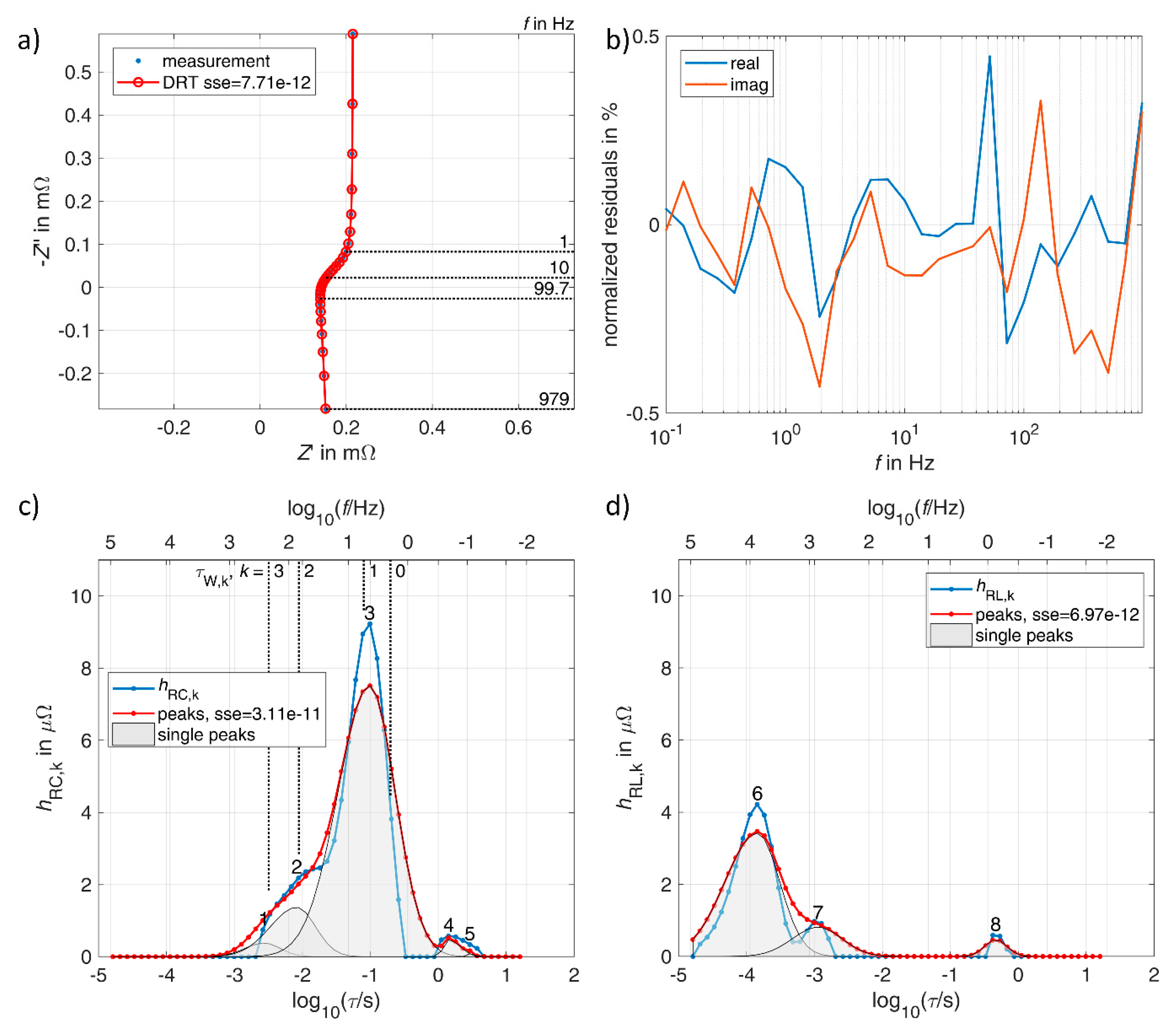
3.2. Vanadium Redox Flow Battery

The power conversion unit of a redox flow battery (RFB) consists of two electrodes separated by an ion-conducting membrane. The energy is stored in two tanks for the anolyte and the catholyte. The two liquids are pumped to the active surface of the electrodes. The prevalent chemistry of RFB is the vanadium redox flow battery (VRFB) that employs vanadium ions in four different oxidation states. The electrolyte in the positive half-cell contains VO 2 + and VO 2 + ions, the electrolyte in the negative half-cell V 3 + and V 2 + ions. The impedance of VRFB is not as extensively studied as that of LIB. Last year, Schneider et al. published a first poster on the DRT analysis of the impedance spectrum of a VRFB [38]. In the following, the same data is used for the GDRT analysis.
The system under study is a VRFB of the producer Micro Flow Cell. The membrane used is fumasep FAP-450 from fumatech, and the electrodes are GFD4.6 from SGL. The impedance spectrum was measured with a minimum frequency of f min = 2   mHz and a maximum frequency of f max = 1   MHz , at 51 measured frequencies in total. The excitation was performed in potentiostatic mode with an excitation signal amplitude of v ^ = 10   mV . Excitation and frequency analysis was conducted by a Gamry Ref 3000 workstation. The cell’s working point was kept constant at a voltage of 1.4   V , corresponding to S O C = 50 % , a flow rate of 25   mL   min 1 , and a temperature of 21   C . For the GDRT analysis the number of predefined time constants was chosen to N τ = 2 N f , with a minimum of τ min   = ( 2 π   f max ) 1 1 decade, and a maximum of τ max = ( 2 π   f min ) 1 + 2 decades.
The calculated DRT spectrum in Figure 5a shows a very good agreement with the measured spectrum with normalized residual values below 1.1% across the whole frequency range as shown in Figure 5b. The identified polarization contributions as listed in Table 5 can be discussed as follows. R Ω is the ohmic resistance mainly due to ionic resistance of ion-conducting membrane, and L is the inductivity of cabling. The converging resistive-capacitive behavior of the impedance spectrum at low frequencies toward the real axis results in no identifiable capacitance C . Five resistive-capacitive contributions were detected in Figure 5c. As for the LIB, a final assignment of peaks 1–5 is possible only by a variation of state variables as state of charge and temperature and by reference electrode measurements. Peak 6 in Figure 5d shows a negligible resistive-inductive contribution at high frequencies. The most remarkable is peak 7, which presents a resistive-inductive contribution at low frequencies, pointing toward mass transport effects of the flow battery. Since the mass flow affects the electrochemical impedance spectrum, it will now be interesting for future work to analyze the direct transfer function of mass flow and cell voltage following the ideas of a generalized application of impedance spectroscopy to different physical domains in the introduction.

3.3. Double Layer Capacitor

Another technical relevant, low ohmic electrochemical system is the double-layer capacitor (DLC) or supercapacitor, especially if the application requires many rapid charge/discharge cycles and high specific power rather than high specific energy. DLCs consist of activated carbon electrodes with a very large active surface. Electrolytes with organic solvents, such as acetonitrile, are used for cells with voltages up to 2.85   V . In literature, the high-frequency impedance and the inductive behavior of double-layer capacitors are often not regarded [39,40].
The system under study is a DLC of the producer Maxwell in a wound cell format with a nominal capacitance of C DLC = 3400   F . The impedance spectrum was measured with a minimum frequency of f min = 100   mHz and a maximum frequency of f max = 1   kHz , at 29 measured frequencies in total. The excitation was performed in potentiostatic mode with an excitation signal amplitude of v ^ = 10   mV . Excitation and frequency analysis was conducted by a Zahner Zennium Pro workstation. The DLC’s working point was kept constant at a voltage of 0.6035   V and a temperature of 30   C . For the GDRT analysis the number of predefined time constants was chosen to N τ = 2 N f , with a minimum of τ min = ( 2 π   f max ) 1 1 decade, and a maximum of τ max = ( 2 π   f min ) 1 + 2 decades.
The calculated DRT spectrum in Figure 6a, again, shows an excellent agreement with the measured spectrum with normalized residual values below 0.5% across the whole frequency range as shown in Figure 6b. The two distribution functions h R C and h R L in Figure 6c,d show less separable processes as the LIB and the RFB. With close peaks or shoulders, the peak analysis reaches its limits, resulting in more overlaying Gauss bells and a lower fitting quality. The identified polarization contributions as listed in Table 6 can be discussed as follows. Analogous to the other electrochemical systems, R Ω is the ohmic resistance mainly due to the ionic resistance of the electrolyte, and L is the inductivity of cabling. Equivalent to the battery’s impedance spectrum, the diverging resistive-capacitive behavior at low frequencies results in an identifiable capacitance C . This variable has to be interpreted as a differential capacity d C Ah / d V of the impedance spectrum [41] and is not to be confused with the nominal capacitance C DLC of the double-layer capacitor measured via a full discharge. Five resistive-capacitive contributions were found in Figure 6c. Peak 1–3 present a characteristic sequence of peaks with falling amplitudes for smaller time constants. The three peaks appear at positions following the same Equation (20) as above. Peak 1–3 can thus be attributed to a single electrode process, even if the electrode process is not diffusion, but rather the resistive-capacitive behavior of a non-ideal double-layer capacitor in parallel to a resistance. A characteristic sequence of peaks at defined relative positions seems to be more general than the derivation presented in [35]. Peaks 4, 5, and 8 show overlapping resistive-capacitive and resistive-inductive contributions that cannot be thoroughly separated at this single measurement. A series of impedance spectra at varying temperatures might help to clarify their origin. Peaks 6–8 in Figure 6d show a complex resistive-inductive behavior that needs further analysis and a more detailed model description of the wound cell format [36].

4. Summary

Electrochemical systems as lithium-ion batteries, redox flow batteries, or double-layer capacitors present complex impedance spectra with ohmic, inductive, capacitive, and resistive-capacitive, as well as resistive-inductive effects. Often, frequency-dependent electrode processes overlap in the Nyquist plot, as illustrated exemplarily in Figure 2a and as shown for the three electrochemical systems tested. Analyzing these spectra by impedance modelling would require major assumptions on the number of polarization processes involved and the nature of the single processes. An analysis of these spectra by examining their distribution or relaxation times was so far limited to resistive-capacitive spectra. Since the most relevant electrode processes are of resistive-capacitive nature a lot of effort was made in literature to exclude non-resistive-capacitive effects off the measured impedance spectra to be able to apply the state of the art DRT analysis. These efforts came along with the price of elaborate modelling and low reproducibility due to a large number of degrees of freedom.
The generalized DRT analysis introduced here now incorporates all relevant impedance behavior in the DRT calculation by identifying two distribution functions for resistive-capacitive and for resistive-inductive effects as well as three lumped parameters for pure ohmic, inductive and capacitive behavior. The GDRT overcomes the need of data preprocessing, i.e., the necessity to model and to reduce measured impedance spectra. The immediate calculation of the GDRT based on measured impedance spectra simplifies the work flow significantly and enables a reliable analysis of complex superposed impedance spectra with unambiguous results and high reproducibility. Since impedance modeling is left out in the work flow of the GDRT, the assumption of DRT being a model-free approach for the characterization of impedance spectra is finally fulfilled. The calculated GDRT spectra show an excellent agreement with the measured spectra with very low normalized residual values across the whole frequency range, including the boundaries of the measured frequency interval.
All arguments considered, the GDRT analysis is a powerful tool to analyze complex impedance spectra with overlapping resistive-capacitive and resistive-inductive polarization contributions by separating the single polarization contributions into two distribution of relaxation times functions, by identifying the number of processes involved without prior assumptions, and finally, by quantifying the single polarization contributions by post-processing of the two distribution functions through peak analysis.

Funding

This research received no external funding.

Acknowledgments

The author thanks Christina Roth (now at University of Bayreuth) and Jonathan Schneider at the Freie Universität Berlin, Germany, for providing the measurement data of the redox flow battery. Thanks to Markus Hahn, Chair of Electrical Energy Systems, University of Bayreuth, Germany, for fruitful discussions and for proof reading the article.

Conflicts of Interest

The authors declare no conflict of interest.

References

  1. Hagen, G.; Schulz, A.; Knörr, M.; Moos, R. Four-Wire Impedance Spectroscopy on Planar Zeolite/Chromium Oxide Based Hydrocarbon Gas Sensors. Sensors 2007, 7, 2681–2692. [Google Scholar] [CrossRef] [PubMed] [Green Version]
  2. Andreaus, B.; McEvoy, A.J.; Scherer, G.G. Analysis of performance losses in polymer electrolyte fuel cells at high current densities by impedance spectroscopy. Electrochim. Acta 2002, 47, 2223–2229. [Google Scholar] [CrossRef]
  3. Danzer, M.A.; Hofer, E.P. Analysis of the electrochemical behaviour of polymer electrolyte fuel cells using simple impedance models. J. Power Sources 2009, 190, 25–33. [Google Scholar] [CrossRef]
  4. Buller, S.; Thele, M.; De Doncker, R.W.A.A.; Karden, E. Impedance-based simulation models of supercapacitors and Li-ion batteries for power electronic applications. IEEE Trans. Ind. Appl. 2005, 41, 742–747. [Google Scholar] [CrossRef]
  5. Andre, D.; Meiler, M.; Steiner, K.; Wimmer, C.; Soczka-Guth, T.; Sauer, D.U. Characterization of high-power lithium-ion batteries by electrochemical impedance spectroscopy. I. Experimental investigation. J. Power Sources 2011, 196, 5334–5341. [Google Scholar] [CrossRef]
  6. Jossen, A. Fundamentals of battery dynamics. J. Power Sources 2006, 154, 530–538. [Google Scholar] [CrossRef]
  7. Tröltzsch, U.; Kanoun, O.; Tränkler, H.-R. Characterizing aging effects of lithium ion batteries by impedance spectroscopy. Electrochim. Acta 2006, 51, 1664–1672. [Google Scholar] [CrossRef]
  8. Schindler, S.; Bauer, M.; Petzl, M.; Danzer, M.A. Voltage relaxation and impedance spectroscopy as in-operando methods for the detection of lithium plating on graphitic anodes in commercial lithium-ion cells. J. Power Sources 2016, 304, 170–180. [Google Scholar] [CrossRef]
  9. Barsoukov, E.; Macdonald, J.R. Impedance Spectroscopy—Theory, Experiment and Applications, 2nd ed.; John Wiley & Sons: Hoboken, NJ, USA, 2005. [Google Scholar]
  10. Baumann, F.S.; Fleig, J.; Habermeier, H.-U.; Maier, J. Impedance spectroscopic study on well-defined (La,Sr)(Co,Fe)O3−δ model electrodes. Solid State Ion. 2006, 177, 1071–1081. [Google Scholar] [CrossRef]
  11. Fleig, J. Solid Oxide Fuel Cell Cathodes: Polarization Mechanisms and Modeling of the Electrochemical Performance. Annu. Rev. Mater. Res. 2003, 33, 361–382. [Google Scholar] [CrossRef]
  12. Heimerdinger, P.; Rosin, A.; Danzer, M.A.; Gerdes, T. Humidity-dependent through-plane impedance technique for proton conducting polymer membranes. Membranes 2019, 9, 62. [Google Scholar] [CrossRef] [PubMed]
  13. Fabregat-Santiago, F.; Bisquert, J.; Palomares, E.; Otero, L.; Kuang, D.; Zakeeruddin, S.M.; Grätzel, M. Correlation between Photovoltaic Performance and Impedance Spectroscopy of Dye-Sensitized Solar Cells Based on Ionic Liquids. J. Phys. Chem. C 2007, 111, 6550–6560. [Google Scholar] [CrossRef]
  14. Garland, J.E.; Crain, D.J.; Zheng, J.P.; Sulyma, C.M.; Roy, D. Electro-analytical characterization of photovoltaic cells by combining voltammetry and impedance spectroscopy: Voltage dependent parameters of a silicon solar cell under controlled illumination and temperature. Energy Env. Sci. 2011, 4, 485–498. [Google Scholar] [CrossRef]
  15. Bertemes Filho, P. Tissue Characterisation using an Impedance Spectroscopy Probe. Ph.D. Thesis, University of Sheffield, Sheffield, UK, 2002. Available online: https://www.researchgate.net/publication/268260305 (accessed on 28 September 2018).
  16. Kyle, U.G.; Bosaeus, I.; De Lorenzo, A.D.; Deurenberg, P.; Elia, M.; Gómez, J.M.; Lilienthal Heitmann, B.; Kent-Smith, L.; Melchior, J.-C.; Pirlich, M.; et al. Bioelectrical impedance analysis—Part I: Review of principles and methods. Clin. Nutr. 2004, 23, 1226–1243. [Google Scholar] [CrossRef] [PubMed]
  17. Bohuslavek, Z. Prediction of commercial classification values of beef carcasses by means of the bioelectrical impedance analysis (BIA). Czech J. Anim. Sci. 2003, 48, 243–250. [Google Scholar]
  18. Gabrielli, C.; Tribollet, B. A Transfer Function Approach for a Generalized Electrochemical Impedance Spectroscopy. J. Electrochem. Soc. 1994, 141, 1147–1157. [Google Scholar] [CrossRef]
  19. Grübl, D.; Janek, J.; Bessler, W.G. Electrochemical Pressure Impedance Spectroscopy (EPIS) as Diagnostic Method for Electrochemical Cells with Gaseous Reactants: A Model-Based Analysis. J. Electrochem. Soc. 2016, 163, 599–610. [Google Scholar] [CrossRef]
  20. Engebretsen, E.; Mason, T.J.; Shearing, P.R.; Hinds, G.; Brett, D.J.L. Electrochemical pressure impedance spectroscopy applied to the study of polymer electrolyte fuel cells. Electrochem. Commun. 2017, 75, 60–63. [Google Scholar] [CrossRef]
  21. Barsoukov, E.; Hwan Jang, J.; Lee, H. Thermal impedance spectroscopy for Li-ion batteries using heat-pulse response analysis. J. Power Sources 2002, 109, 313–320. [Google Scholar] [CrossRef]
  22. Schmidt, J.P.; Manka, D.; Klotz, D.; Ivers-Tiffée, E. Investigation of the thermal properties of a Li-ion pouch-cell by electrothermal impedance spectroscopy. J. Power Sources 2011, 196, 8140–8146. [Google Scholar] [CrossRef]
  23. Klotz, D.; Shai Ellis, D.; Dotan, H.; Rothschild, A. Empirical in operando analysis of the charge carrier dynamics in hematite photo anodes by PEIS, IMPS and IMVS. Phys. Chem. Chem. Phys. 2016, 18, 23438–23457. [Google Scholar] [CrossRef] [PubMed]
  24. Ivers-Tiffée, E.; Weber, A. Evaluation of electrochemical impedance spectra by the distribution of relaxation times. J. Ceram. Soc. Jpn. 2017, 125, 193–201. [Google Scholar] [CrossRef] [Green Version]
  25. Schichlein, H.; Müller, A.C.; Voigts, M.; Krügel, A.; Ivers-Tiffée, E. Deconvolution of electrochemical impedance spectra for the identification of electrode reaction mechanisms in solid oxide fuel cells. J. Appl. Electrochem. 2002, 32, 875–882. [Google Scholar] [CrossRef]
  26. Illig, J.; Ender, M.; Chrobak, T.; Schmidt, J.P.; Klotz, D.; Ivers-Tiffée, E. Separation of charge transfer and contact resistance in LiFePO4-cathodes by impedance modeling. J. Electrochem. Soc. 2012, 159, 952–960. [Google Scholar] [CrossRef]
  27. Schmidt, J.P.; Berg, P.; Schönleber, M.; Weber, A.; Ivers-Tiffée, E. The distribution of relaxation times as basis for generalized time-domain models for Li-ion batteries. J. Power Sources 2013, 221, 70–77. [Google Scholar] [CrossRef]
  28. Weiß, A.; Schindler, S.; Galbiati, S.; Danzer, M.A.; Zeis, R. Distribution of Relaxation Times Analysis of High-Temperature PEM Fuel Cell Impedance Spectra. Electrochim. Acta 2017, 230, 391–398. [Google Scholar] [CrossRef]
  29. Rosenbach, D.; Mödl, N.; Hahn, M.; Petry, J.; Danzer, M.A.; Thelakkat, M. Synthesis and Comparative Studies of Solvent-free Brush Polymer Electrolytes for Lithium Batteries. ACS Appl. Energy Mater. 2019. [Google Scholar] [CrossRef]
  30. Hahn, M.; Schindler, S.; Triebs, L.-C.; Danzer, M.A. Optimized Process Parameters for a Reproducible Distribution of Relaxation Times Analysis of Electrochemical Systems. Batteries 2019, 5, 43. [Google Scholar] [CrossRef]
  31. Tikhonov, A.N. On the stability of inverse problems. Dokl. Akad. Nauk SSSR 1943, 39, 195–198. [Google Scholar]
  32. Weese, J. A reliable and fast method for the solution of Fredholm integral equations of the first kind based on Tikhonov regularization. Comput. Phys. Commun. 1992, 69, 99–111. [Google Scholar] [CrossRef]
  33. Tikhonov, A.N.; Goncharsky, A.; Stepanov, V.; Yagola, A.G. Numerical Methods for the Solution of Ill-Posed Problems; Springer Science & Business Media: Berlin, Germany, 2013. [Google Scholar]
  34. Lawson, C.L.; Hanson, R.J. Solving Least-Squares Problems; Prentice Hall: Upper Saddle River, NJ, USA, 1974; Chapter 23; p. 161. [Google Scholar]
  35. Boukamp, B.A.; Rolle, A. Analysis and Application of Distribution of Relaxation Times in Solid State Ionics. Solid State Ion. 2017, 302, 12–18. [Google Scholar] [CrossRef]
  36. Schindler, S.; Danzer, M.A. Influence of cell design on impedance characteristics of cylindrical lithium-ion cells: A model-based assessment from electrode to cell level. J. Energy Storage 2017, 12, 157–166. [Google Scholar] [CrossRef]
  37. Boukamp, B.A. Derivation of a Distribution Function of Relaxation Times for the (fractal) Finite Length Warburg. Electrochim. Acta 2017, 252, 154–163. [Google Scholar] [CrossRef]
  38. Schneider, J.; Zeis, R.; Danzer, M.A.; Roth, C. Employing DRT Analysis in VRFB: Towards Online Degradation Monitoring. In Proceedings of the Electrochemistry 2018, Ulm, Germany, 24–26 September 2018. [Google Scholar]
  39. Itagaki, M.; Suzuki, S.; Shitanda, I.; Watanabe, K.; Nakazawa, H. Impedance analysis on electric double layer capacitor with transmission line model. J. Power Sources 2007, 164, 415–424. [Google Scholar] [CrossRef]
  40. Yoo, H.D.; Jang, J.H.; Ryu, J.H.; Park, Y.; Oh, S.M. Impedance analysis of porous carbon electrodes to predict rate capability of electric double-layer capacitors. J. Power Sources 2014, 267, 411–420. [Google Scholar] [CrossRef]
  41. Schönleber, M.; Ivers-Tiffée, E. The Distribution Function of Differential Capacity as a new tool for analyzing the capacitive properties of Lithium-Ion batteries. Electrochem. Commun. 2015, 61, 45–48. [Google Scholar] [CrossRef]
Figure 1. Dynamic, frequency dependent processes of an electrochemical system (in green) and battery test methods (in blue) with typical ranges of characteristic time constants.
Batteries 05 00053 g001
Figure 2. Example spectrum of series connection of an ohmic resistance, an RC element, and a ZARC element. (a) Nyquist plot of the spectrum with the sum of squared errors ( s s e ) according to Equation (5); (b) Distribution of relaxation times h k of the spectrum with fitted peaks and the sum of squared errors of their residual. In legends the engineering notation is used for s s e values, where, e.g., 1.62e-08 corresponds to 1.62 10 8 .
Batteries 05 00053 g002
Figure 3. (a) Work flow of state of the art DRT analysis with two model-based steps for preprocessing measured impedance data to extract the resistive-capacitive behavior of the measured spectrum; (b) Reduced work flow of model-free generalized DRT analysis without the need of data preprocessing resulting in two distribution functions of relaxation times, one for the resistive-capacitive behavior and one for the resistive-inductive behavior.
Batteries 05 00053 g003
Figure 4. Generalized DRT analysis of a lithium-ion battery (A123 Systems, LFP-graphite, 2.6 Ah, 26650) with the sum of squared errors ( s s e ) of each plot. (a) Measured and calculated impedance spectrum; (b) Normalized residuals of real and imaginary part of the impedance spectra of subplot (a); (c) Identified resistive-capacitive distribution of relaxation times function; (d) Identified resistive-inductive distribution of relaxation times function.
Batteries 05 00053 g004
Figure 5. Generalized DRT analysis of a vanadium redox-flow battery (Micro Flow Cell, Separator Nafion, Electrodes SGL GFA6) with the sum of squared errors ( s s e ) of each plot. (a) Measured and calculated impedance spectrum; (b) Normalized residuals of real and imaginary part of the impedance spectra of subplot (a); (c) Identified resistive-capacitive distribution of relaxation times function; (d) Identified resistive-inductive distribution of relaxation times function.
Batteries 05 00053 g005
Figure 6. Generalized DRT analysis of a double layer capacitor (Maxwell, 3400 F, 2.85 V) with the sum of squared errors ( s s e ) of each plot. (a) Measured and calculated impedance spectrum; (b) Normalized residuals of real and imaginary part of the impedance spectra of subplot (a); (c) Identified resistive-capacitive distribution of relaxation times function; (d) Identified resistive-inductive distribution of relaxation times function.
Batteries 05 00053 g006
Table 1. Generalized impedances of different physical domains in analogy to the standard impedance definition of the electrical domain.
Physical DomainGeneralized Voltage (Intensive, Across Variable)Generalized Current (Extensive, Through Variable)Generalized Impedance (Transfer Function)
ElectricalVoltage V Current I Impedance Z
ElectrostaticVoltage V Dielectric flow ϕ D Dielectric impedance Z D
MagnetostaticMagnetic voltage V m Magnetic flow ϕ B Magnetic resistance Z m
Mechanical (translatory)Force F Velocity v Mass m
Mechanical (rotatory)Torque M Angular velocity ω Inertia J
Hydro-mechanicalPressure p Volume flow V ˙ , Mass flow m ˙ Pneumatic impedance Z p
Thermal conductivityTemperature difference Δ T Heat flow W Thermal impedance Z T
Table 2. Model parameter values of the impedance simulation of series connection of an ohmic resistance, an RC element, and a ZARC element.
Impedance ElementParameterValue
Ohmic resistance R Ω 3   m Ω
RC element R 1 4   m Ω
τ 1 0.5   ms
ZARC element R 2 7   m Ω
τ 2 5   ms
φ 2 0.8
Table 3. Degrees of freedom and variables of distribution of relaxation times (DRT) calculation.
Degree of FreedomVariable
Definition of error and optimization function e ,   J ,   min h k { J }
Modelling of impedance spectrum Z EIS , mod
Exclusion of non-resistive-capacitive elements Z reduced = Z meas Z mod ,   excl
Number of time constants N τ
Min/max time constant τ min ,   τ max
Distribution of predefined time constants [ τ min τ k τ max ]
Choice of regularization parameter λ
Table 4. Identified polarization contributions of the lithium-ion battery comprising ohmic resistance, inductivity, capacitance, resistive-capacitive, and resistive-inductive elements.
VariableValueVariableValue
R Ω 7.97   m Ω
L 29.3   nH
C 854   mF
R 1 6.35   m Ω τ 1 58.7   μ s
R 2 1.41   m Ω τ 2 421   μ s
R 3 1.55   m Ω τ 3 2.29   ms
R 4 2.43   m Ω τ 4 13.5   ms
R 5 0.499   m Ω τ 5 99.5   ms
R 6 1.03   m Ω τ 6 455   ms
R 7 3.22   m Ω τ 7 2.97   s
R 8 1.41   m Ω τ 8 9.20   μ s
Table 5. Identified polarization contributions of the vanadium redox-flow battery comprising ohmic resistance, inductivity, capacitance, resistive-capacitive, and resistive-inductive elements.
VariableValueVariableValue
R Ω 160   m Ω
L 223   nH
C 0   mF
R 1 42.9   m Ω τ 1 28.8   μ s
R 2 30.5   m Ω τ 2 272   μ s
R 3 252   m Ω τ 3 2.46   ms
R 4 14.9   m Ω τ 4 31.8   ms
R 5 16.7   m Ω τ 5 1.39   s
R 6 1.10   m Ω τ 6 4.99   μ s
R 7 35.1   m Ω τ 7 5.45   s
Table 6. Identified polarization contributions of the double-layer capacitor comprising ohmic resistance, inductivity, capacitance, resistive-capacitive, and resistive-inductive elements.
VariableValueVariableValue
R Ω 7.97   m Ω
L 29.3   nH
C 854   mF
R 1 6.35   m Ω τ 1 58.7   μ s
R 2 1.41   m Ω τ 2 421   μ s
R 3 1.55   m Ω τ 3 2.29   ms
R 4 2.43   m Ω τ 4 13.5   ms
R 5 0.499   m Ω τ 5 99.5   ms
R 6 1.03   m Ω τ 6 455   ms
R 7 3.22   m Ω τ 7 2.97   s
R 8 1.41   m Ω τ 8 9.20   μ s

