Optimized Process Parameters for a Reproducible Distribution of Relaxation Times Analysis of Electrochemical Systems

Abstract

The distribution of relaxation times (DRT) analysis offers a model-free approach for a detailed investigation of electrochemical impedance spectra. Typically, the calculation of the distribution function is an ill-posed problem requiring regularization methods which are strongly parameter-dependent. Before statements on measurement data can be made, a process parameter study is crucial for analyzing the impact of the individual parameters on the distribution function. The optimal regularization parameter is determined together with the number of discrete time constants. Furthermore, the regularization term is investigated with respect to its mathematical background. It is revealed that the algorithm and its handling of constraints and the optimization function significantly determine the result of the DRT calculation. With optimized parameters, detailed information on the investigated system can be obtained. As an example of a complex impedance spectrum, a commercial Nickel–Manganese–Cobalt–Oxide (NMC) lithium-ion pouch cell is investigated. The DRT allows the investigation of the SOC dependency of the charge transfer reactions, solid electrolyte interphase (SEI) and the solid state diffusion of both anode and cathode. For the quantification of the single polarization contributions, a peak analysis algorithm based on Gaussian distribution curves is presented and applied.

1. Introduction

Electrochemical impedance spectroscopy (EIS) is a well-known method applied since the 1970s [1] for electrochemical power sources and their components including materials such as commercial battery cells [2], single electrodes [3,4], experimental cells with reference electrodes [5], solid oxide fuel cells (SOFCs) [6], polymer membrane fuel cells (PEMFCs) [7], separators, membranes or electrolytes [8,9]. In addition, the technique is used in other scientific fields, e.g., to obtain the bio impedance in medicine [10] or biology.

The EIS provides the frequency-dependent impedance of an electrochemical system by applying a sinusoidal current, measuring the voltage response (galvanostatic EIS) or vice versa (potentiostatic EIS), and applying Ohm’s law. The impedance spectra are interpreted regarding their high-frequency inductive behavior [11] caused by geometry, wiring and the test setup, their low-frequency diffusion behavior [12] and mainly their interphase behavior. Numerous studies focus on battery impedance, e.g., correlating aging to changes in the impedance spectrum [13] or explaining the relaxation behavior in graphite anodes [14]. Analyzing the impedance without applying further techniques is complex, though. Effects overlap, processes are non-ideal, causing deviations between the expected and the measured spectra. Even the number of single processes cannot be obtained unambiguously. Therefore, the DRT became of interest in the 1990s [1] and was applied first for SOFCs [15,16]. Later on, the DRT was adapted for the characterization of PEMFC and batteries [2,7,17]. As the result of a mathematical transformation, the polarization contributions at predefined time constants of the investigated system are derived. 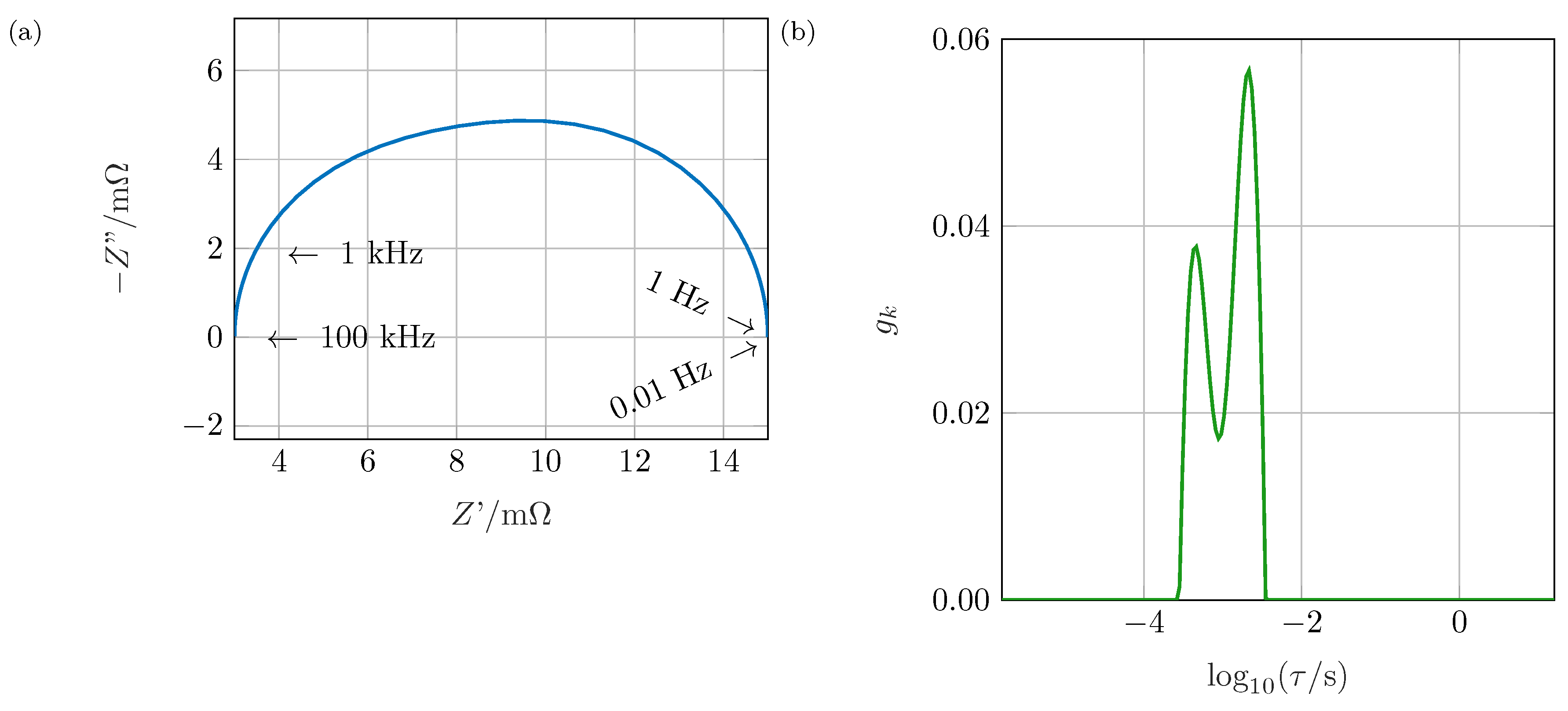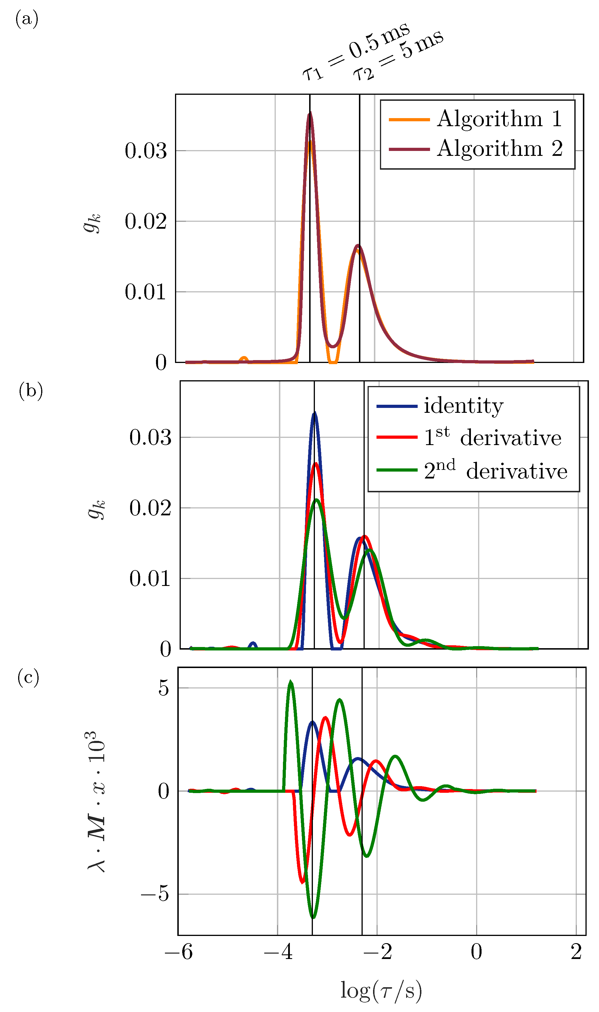Exemplary, in Figure 1a the impedance spectrum of two RC elements (resistor and capacitor in parallel) connected in series is shown: a deformed semi-circle with no distinct maximum of $-Im\left(\mathrm{Z}\right)$ results. This shape might be caused, e.g., by a non-ideal process due to large inhomogeneities within the electrode or by separate processes. Investigating the impedance spectrum, no further conclusions can be drawn. Applying the DRT algorithm as shown in Figure 1b, the two involved processes can be separated easily. Therefore, the contribution of single processes to the system’s impedance can be calculated.

The DRT offers a model-free, universal approach for the detailed analysis of electrochemical systems or any other data obtained from impedance measurement. This means that no a-priori assumptions, e.g., electrical, physical or chemical models or knowledge are necessary, which is an essential advantage when dealing with complex or hardly understood specimen such as fuel cell stacks or new materials with novel conducting mechanisms.

On the other hand, the DRT analysis strongly depends on the choice of its process parameters which are, in many publications, neither revealed nor discussed. Thus, the DRT algorithm containing those parameters is described in detail within this paper. Furthermore, an extensive parameter study is performed to evaluate the impact and correlation of those process parameters on the calculated distribution function. The study includes the optimization of the regularization parameter, the number of predefined discrete time constants as sampling points of the distribution function and the mathematical formulation of the regularization term. It is investigated whether real parts, imaginary parts of the complex impedance or both should be used for the calculation of the DRT. Finally, the impact of the optimization function and optimization algorithm is shown. As an instructive example of a complex impedance spectrum comprising inductive, resistive, capacitive and diffusive overlapping polarization contributions of multiple components within an electrochemical system, the algorithm is applied on impedance data from a commercial $3.3$ Ah Nickel–Manganese–Cobalt–Oxide (NMC) lithium-ion pouch cell by Kokam and the results are discussed in detail. Furthermore, the features of the impedance spectra are assigned to the individual peaks observed in the distribution functions. For more insight into the single peaks within the DRT, a novel post-processing approach is presented, adapting modified Gaussian peaks to the distribution function resulting in a quantification of every single process within the spectrum.

By reporting all relevant information about the used algorithm, the results presented in this publication can be easily reproduced by other researchers. The information includes

• the optimization algorithm,
• the error function,
• the type of data used, i.e., using real or imaginary parts of the complex impedance,
• measurement parameters, e.g., current or frequency range,
• regularization parameter,
• number of time constants,
• the pre- and post-processing routine,
• the minimum and maximum time constants for the DRT.

2. Deriving DRT from EIS Data

The main idea of the DRT is to express the complex-valued, frequency-dependent impedance of an electrochemical system as an infinite series of differential RC-elements in series with an ohmic resistor $R_0$ [7,15,17]:

$$\begin{array}{c}\hfill Z\left(j\omega \right)=R_0+{\int }_0^{\infty }\frac{h\left(\tau \right)}{1+j\omega \tau }\mathrm{d}\tau .\end{array}$$

(1)

The integral is often normalized by introducing

$$\begin{array}{c}\hfill {\int }_0^{\infty }g\left(\tau \right)\mathrm{d}\tau =1,\end{array}$$

(2)

which leads to

$$\begin{array}{c}\hfill Z\left(j\omega \right)=R_0+R_{\mathrm{pol}}·{\int }_0^{\infty }\frac{g\left(\tau \right)}{1+j\omega \tau }\mathrm{d}\tau .\end{array}$$

(3)

The normalized Equation (3) has two advantages compared to Equation (1):

• The total polarization resistance of the system gets apparent by $R_{\mathrm{pol}}$.
• Systems with impedances in different orders of magnitude can be compared easily.

The term $\frac{g\left(\tau \right)}{1+j\omega \tau }$ corresponds to the relative differential contribution of a single ohmic-capacitive element as $\tau =RC$ and $g\left(\tau \right)=MMR/R_{\mathrm{pol}}$ results in $\frac{R}{1+j\omega RC}$, which is the well-known equation for an RC-element.

The function $g\left(\tau \right)$ is computed numerically. Therefore, the integral in Equation (3) has to be discretized yielding the finite sum

$$\begin{array}{c}\hfill Z\left(j\omega \right)=R_0+R_{\mathrm{pol}}·\sum _{k=1}^n\frac{g\left({\tau }_k\right)}{1+j\omega {\tau }_k}.\end{array}$$

(4)

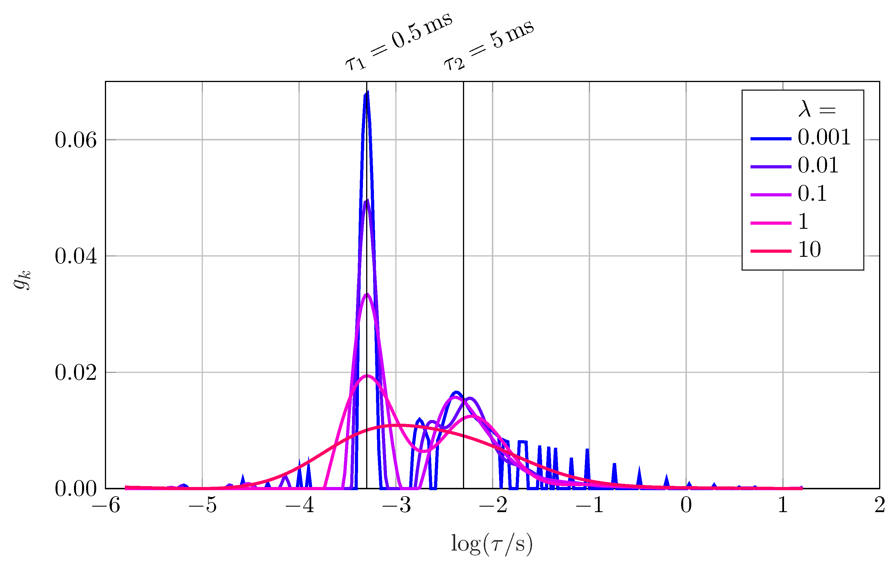
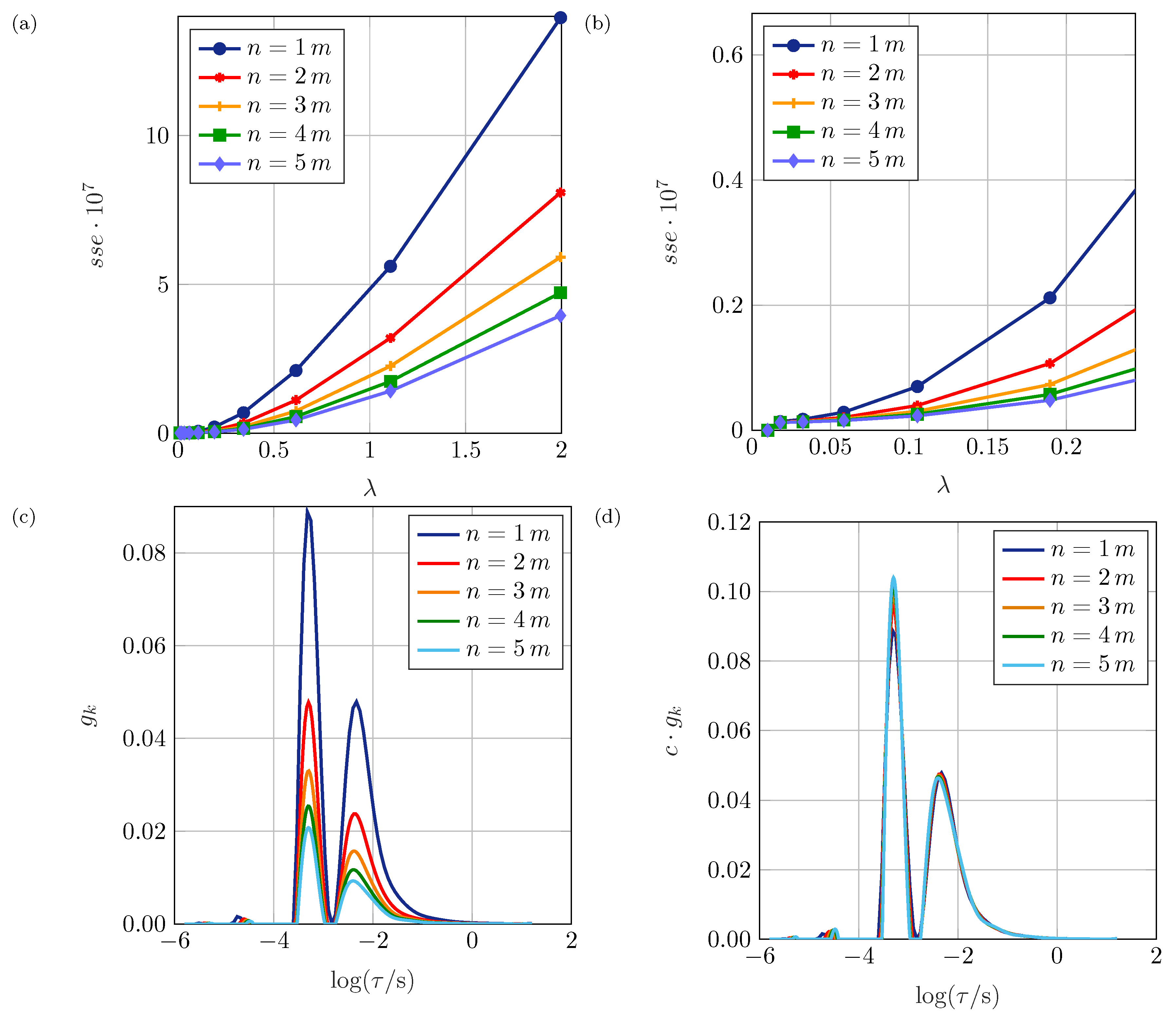
The range of time constants $[{\tau }_1,{\tau }_n]$ has to be chosen a priori based on the available frequency range of the impedance data. Usually, the interval of time constant matches the interval of measured frequencies. The number of time constants n has to be large compared to the expected numbers of processes within the investigated system. The determination of the optimal number is part of our process parameter analysis in Section 3.

Equation (4) describes the resistive–capacitive behavior of the impedance spectrum as a sum of RC elements connected in series with predefined time constants. Neither assumptions are made regarding the number of processes involved nor model concepts on electrical, physical or chemical processes are required as in case of the model-based analysis of electrochemical impedance spectroscopy. Hence, the DRT analysis is regarded as a model-free method for the characterization of electrochemical systems. Furthermore, it has to be stated that due to the ohmic-capacitive nature of Equation (4), the DRT is not valid for inductive systems. Purely capacitive contributions cannot be described neither. Mathematically, these restrictions regarding the examined complex impedance can be expressed as

$$\begin{array}{cc}\hfill \underset{\omega \to 0}{lim}Im\left(Z\right(j\omega \left)\right)& \stackrel{!}{=}0\hfill \end{array}$$

(5)

$$\begin{array}{cc}\hfill \underset{\omega \to \infty }{lim}Im\left(Z\right(j\omega \left)\right)& \stackrel{!}{=}0\hfill \end{array}$$

(6)

$$\begin{array}{cc}\hfill Im\left(Z\right(j\omega \left)\right)& \stackrel{!}{\le }0\forall \omega .\hfill \end{array}$$

(7)

2.1. Dealing with Artefacts at the Boundaries of the Measured Frequency Range

If the measured impedance spectrum is not converging towards the real axis at the boundaries of the measured frequency range as demanded by Equations (5) and (6), as is it the case e.g., for diffusion processes at low frequencies, the DRT analysis will yield artefacts, i.e., singularities or diverging, steep slopes at the boundaries of the interval of time constants corresponding to the extremes of the measured frequencies. To deal with this issue we propose to extend the predefined vector of time constants beyond the minimum or maximum time constant corresponding to the according maximum and minimum frequency. Mathematically this is legitimate since the choice of the predefined time constants does not have to match the measured frequencies compulsorily as can be seen in the definition of the optimization problem later. This approach does not extrapolate the measured spectrum beyond the measured frequency range. Not even new assumptions are made on the behavior of the device under test beyond the measured frequency range. Instead, the optimization problem maps a wider vector of time constants onto the exactly same impedance information in frequency domain and therewith helps to better extract all information contained in the measured frequency spectrum. A back calculation of the identified DRT into frequency domain would be the same as fitting an RC circuit to the measured spectrum. As for fitting an equivalent circuit model to a measured impedance spectrum, the model is only valid for the measured frequency range. Since real systems will never have a limited bandwidth and a measurement system will never be able to measure an unlimited frequency range, we show in the results that broadening the predefined vector of time constants is beneficial for the analysis of electrochemical systems, especially if polarization processes are not abated at the boundaries of the measured frequencies as it the case for the solid state diffusive behavior of lithium-ion batteries.

2.2. Calculation of g($\tau$)

For the equations above, $g\left(\tau \right)$ has to be calculated from an impedance spectrum. Measured or model-based, computer-generated spectra are limited in their number of frequency points. Typically, the frequency vector of the treated impedance data is logarithmically scaled, with 6 [14], 7 [18], 10 [7,19] or 16 [20] steps per decade, respectively. Often, this information is missing in publications [2,21,22]. However, this relatively small amount of m data points (i.e., the measured data including frequency and impedance values) leads to the issue that there are usually less data points than sampling points for the time constants of the DRT analysis ($m<n$).

Therefore, the resulting optimization problem

$$\begin{array}{c}\hfill \min \left\{\left|\right|\mathbf{A}\mathbf{x}-\mathbf{b}|{|}^2\right\},\end{array}$$

(8)

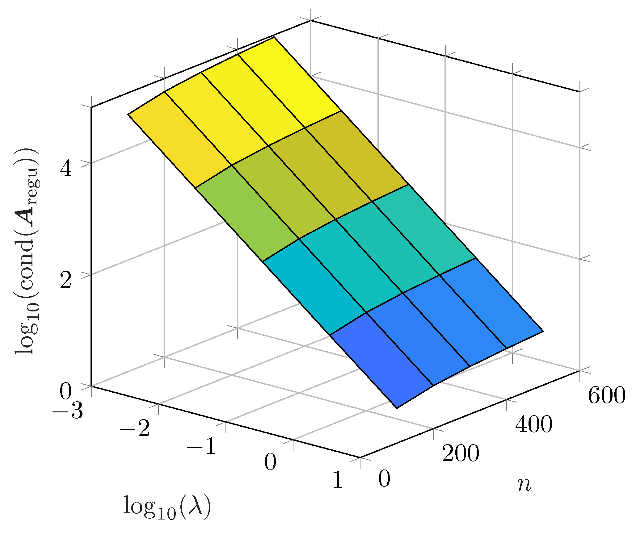
with the matrix $\mathit{A}$ and the vector $\mathit{b}$ as introduced below is ill-posed and might be ill-conditioned. Therefore, it cannot be solved analytically. One way to overcome the ill-posed optimization problem in Equation (8) is to apply numerical regularization. Among the regularization techniques commonly used for calculation of DRTs of electrochemical systems, Tikhonov regularization has proven to be a powerful technique [23,24]. The optimization function

$$\begin{array}{c}\hfill \min \left\{\left|\right|\mathbf{A}\mathbf{x}-\mathbf{b}|{|}^2+|\left|\lambda \mathbf{x}\right|{|}^2\right\}\end{array}$$

(9)

is extended by a regularization term ${\left|\right|\lambda \mathit{x}\left|\right|}^2$ where $\lambda$ is the regularization parameter. Its influence on the resulting distribution will be discussed in Section 3. The parameter $\mathit{x}$ represents the discrete values of the distribution function $g\left(\tau \right)$.

The parameter $\lambda \mathit{x}$ can be extended to $\mathit{M}·\lambda \mathit{x}$, where $\mathit{M}$ is the regularization matrix. In the simplest case, $\mathit{M}$ is defined as $\mathit{I}$, representing the $n\times n$ identity matrix.

In addition, the constraint

$$\begin{array}{c}\hfill x_k=g\left({\tau }_k\right)\ge 0\forall k,0<k\le n\end{array}$$

(10)

has to be taken into account, since negative contributions to the impedance are physically not feasible.

The solution of the problem stated in Equation (9) can be obtained by multiple numeric algorithms. As the optimization problem is ill-posed with no unique solution and as commonly used least-squares algorithms are only able to find local optima, it is crucial to be aware of the used optimization algorithm. Otherwise, the results of the DRT can hardly be reproduced. Ciucci et al. [25] and Wan et al. [26] give insight into the optimization problem including a detailed discussion on the regularization matrix. Nevertheless, to the authors’ knowledge there is no publication which gives insight into the used optimization algorithm.

Considering Equation (4), the matrix $\mathit{A}$ consists of $A_{i,k}$ in i-th line and k-th column where

$$\begin{array}{c}\hfill A_{i,k}=\frac{1}{1+j{\omega }_i{\tau }_k}\end{array}$$

(11)

represent normalized RC-elements with a time constant ${\tau }_k$ evaluated at the angular frequency ${\omega }_i$.

The vector $\mathit{b}$ consists of the m measured or generated impedance values. This may happen in various ways:

• Using complex values:

  $$\begin{array}{c}\hfill \mathbf{A}=\left[\begin{array}{cccc}{A}_{1,1}& A_{1,2}& \cdots & A_{1,n}\\ A_{2,1}& A_{2,2}& \cdots & A_{2,n}\\ ⋮& ⋮& \ddots & ⋮\\ A_{m,1}& A_{m,2}& \cdots & A_{m,n}\end{array}\right],\mathbf{b}=\left[\begin{array}{c}{Z}_{\mathrm{meas},1}\\ Z_{\mathrm{meas},2}\\ ⋮\\ Z_{\mathrm{meas},m}\end{array}\right].\end{array}$$

  (12)
  In this case, a solver is needed which is able to handle complex values as well as constraints.
• Using the real parts only:

  $$\begin{array}{c}\hfill \mathbf{A}=\left[\begin{array}{ccc}Re\left(A_{1,1}\right)& \cdots & Re\left(A_{1,n}\right)\\ ⋮& \ddots & ⋮\\ Re\left(A_{m,1}\right)& \cdots & Re\left(A_{m,n}\right)\end{array}\right],\mathbf{b}=\left[\begin{array}{c}Re\left(Z_{\mathrm{meas},1}\right)\\ ⋮\\ Re\left(Z_{\mathrm{meas},m}\right)\end{array}\right].\end{array}$$

  (13)
  Ignoring imaginary parts is legitimate due to the Kramers–Kronig relationship [27,28], as long as its conditions are fulfilled. It can be assumed that a properly measured spectrum complies with these. The linear Kramers–Kronig test is one option to prove the Kramers–Kronig validity of the examined impedance data.
• Using the imaginary parts only: equivalent to Equation (13) substituting real parts by imaginary parts.
• Using both real and imaginary parts:

  $$\begin{array}{c}\hfill \mathbf{A}=\left[\begin{array}{ccc}Re\left(A_{1,1}\right)& \cdots & Re\left(A_{1,n}\right)\\ ⋮& \ddots & ⋮\\ Re\left(A_{m,1}\right)& \cdots & Re\left(A_{m,n}\right)\\ Im\left(A_{1,1}\right)& \cdots & Im\left(A_{1,n}\right)\\ ⋮& \ddots & ⋮\\ Im\left(A_{m,1}\right)& \cdots & Im\left(A_{m,n}\right)\end{array}\right],\mathbf{b}=\left[\begin{array}{c}Re\left(Z_{\mathrm{meas},1}\right)\\ ⋮\\ Re\left(Z_{\mathrm{meas},m}\right)\\ Im\left(Z_{\mathrm{meas},1}\right)\\ ⋮\\ Im\left(Z_{\mathrm{meas},m}\right)\end{array}\right],\end{array}$$

  (14)

  which provides more, in case of a noise-free measurement redundant, information. If not stated otherwise, this method is used within this publication.

With both real and imaginary parts used, a number of time constants $n>2\times m$ leads to an under-determined system. With $n<2\times m$, the problem is overdetermined. Both cases lead to an ill-posed problem as there is no unique solution. If $n=2\times m$, the system is well-posed. For all three cases, Tikhonov regularization is applicable.

A non-negative least squares (NNLS) solver is used as proposed by Lawson and Hanson ([29], p. 161). As this algorithm can only deal with matrix-vector-systems, Equation (9) is re-written according to Kaipio [30] and Wu [31]:

$$\begin{array}{c}\hfill A_{\mathrm{Reg}}=\left[\begin{array}{c}A\\ \lambda ·I\in {\mathbb{R}}^{n\times n}\end{array}\right]b_{\mathrm{Reg}}=\left[\begin{array}{c}b\\ 0\in {\mathbb{R}}^n\end{array}\right].\end{array}$$

(15)

The solver returns $h\left({\tau }_k\right)$ which turns into $g\left({\tau }_k\right)$ after normalization.

2.3. Pre-Processing of Measurement Data

As stated above, the DRT can only deal with resistive–capacitive systems. The frequency- independent $R_0$ has to be subtracted from the impedance before running the DRT routine. In addition, electrochemical systems are never only resistive–capacitive. There are inductive contributions due to the measurement setup or the specimen itself [11] as well as diffusive behavior e.g., when investigating batteries. Therefore, it is critical that such influences are removed from the impedance data beforehand.

There are two proper ways to deal with inductive and capacitive branches: the first is to fit an appropriate equivalent circuit (EC) to the measurement data using the model-and-reduce approach. This EC may contain a resistor, an inductor, a capacitor, RL-elements (resistor and inductivity in parallel), RC-elements, ZARC-elements ($Z_{\mathrm{ZARC}}=\frac{R}{1+{\left(j\omega RC\right)}^{\phi }}$), constant phase elements (CPE) ($Z_{\mathrm{CPE}}=\frac{1}{1+{\left(j\omega \right)}^{\phi }C}$) and Warburg-elements (planar and spherical diffusion) all connected in series. The contribution of non-resistive–capacitive EC elements is subtracted from the measured spectrum to fulfil the RC-constraint of the DRT (Equations (5)–(7))

This pre-processing step is in opposition to the advantage of not needing any a priori knowledge for the DRT at first glance as the EC fit needs to be precise. Only non-RC elements have to be identified and characterized precisely to be subtracted properly while the exact characterization of electrode and interface processes is not essential within this step. Imprecise EC fits lead to peaks without any physical meaning, offering space for misinterpretations. For an appropriate fit, Equations (5) and (6) should be fulfilled after subtracting non-inductive-resistive components.

Choosing an EC requires experience by the scientist. A by-inspection analysis of the impedance spectrum while keeping in mind the spectra of the specific elements is beneficial. The EC is then fitted using a trust-region method. The two-dimensional error function to be minimized is given by

$$\begin{array}{c}\hfill e=\left[\begin{array}{c}(Re\left(Z\right)-Re\left(Z_{\mathrm{mod}}\right))/|Z|\\ (Im\left(Z\right)-Im\left(Z_{\mathrm{mod}}\right))/|Z|\end{array}\right],\end{array}$$

(16)

with $Z_{\mathrm{mod}}$ representing the impedance function of the EC whose parameters are to be optimized.

The second option, called cut-and-shift approach, does not need any a priori assumptions: first, all data points with $Im\left(Z\right)>0$ are cut off the spectrum. As a second step, the ohmic offset is removed by subtracting $R_0=min\{Re\left(Z\right)\}$ from the spectrum.

The entire workflow is summarized in Figure 2. The validity of the measured spectrum is proven by Kramers–Kronig test: in accordance to literature, a spectrum is said to be valid as long as the residual between the measured and the Kramers–Kronig reconstructed impedance is below 1% for every data point. Within the pre-processing step non-resistive–capacitive components are removed. Finally, the DRT is calculated from the reduced spectrum and $g\left({\tau }_k\right)$ is obtained.

Tikhonov regularization is not the only possible approach for calculating the DRT. Fourier transformation is used as well [15,17]. A comparison between regularization and Fourier transform is not part of this paper, though a study on benefits and disadvantages of either method might be interesting in the future.

2.4. Post-Processing of Result

In general, once $g\left({\tau }_k\right)$ has been calculated, the distribution function can simply be interpreted in a phenomenological manner: the number of processes involved can be identified as well as changes e.g., during ageing or relaxation or differences between used materials, morphologies or cell designs. For a proper quantitative analysis, post-processing is required.

We quantify the polarization of each peak by fitting the numerical distribution to a sum of modified, non-normalized Gaussian probability density functions with adjustable height H, standard deviation $\sigma$ and skew s using a logarithmic time constants scale. The introduction of the skew allows asymmetric distributions:

$$\begin{array}{c}\hfill H·exp\left\{-\frac{({log}_{10}\tau -{log}_{10}{\tau }_0)·\left[1+sgn({log}_{10}\tau -{log}_{10}{\tau }_0)·s\right]}{2·{\sigma }^2}\right\}.\end{array}$$

(17)

Thus, the area under each specific peak corresponds to the impedance contribution of the underlying process. Furthermore, the standard deviation corresponds to the ideality or uniformity of a process, e.g., a narrow peak indicates a process with a small band width, e.g., a uniform particle size. Wide peaks point to distributed processes, e.g., a wide spread particle size distribution or a geometric influence of a large-scale specimen. The skew indicates the distribution of the non-ideal process, e.g., whether there are more small-sized or large particles within the electrode. Yet, an overall quantification or correlation to the system’s attributes is not easily achievable, but a quantitative comparison between various DRTs can be achieved.

The entire algorithm, as described within this chapter, is available for download at http://www.ec-idea.uni-bayreuth.de.

3. Analysis of DRT Process Parameters

3.1. Regularization Parameter and Number of Time Constants

For reliable and meaningful results, the regularization parameter $\lambda$ and the number of time constants n have to be chosen adequately. In Equation (9), the condition $\lambda >0$ forces $\mathit{x}$ towards small $\left|\right|\mathit{x}\left|\right|$ as a direct consequence of the minimization problem. Other publications have noted that an increase of $\lambda$ results in a smoother shape of the DRT. This might lead to the risk that narrow peaks merge or small peaks disappear while small $\lambda$ may cause oscillations or peaks with no physical meaning [7,32,33]. It is intuitive that small values of $\left|\right|\mathit{x}\left|\right|$ lead to a smoother shape of $g_k$ and vice versa. Small $\left|\right|\mathit{x}\left|\right|$ are achieved by a vector whose elements differ little, as outliers deteriorate the norm in the second order.

The expectations from literature are perfectly matched by the results shown in Figure 3. For small $\lambda$, oscillations occur for low time constants and around the second peak. If $\lambda$ is chosen too large, the two peaks begin to merge and cannot be separated anymore. Furthermore, the amplitude decreases while the width of the peaks increases. The total area below the graphs does not change significantly. Several publications were dealing with the issue of optimizing the regularization parameter for their purposes. For this study, we investigated three approaches made by Saccoccio et al. [34] and Hansen [35]: using the so-called discrepancy method, the term

$$\begin{array}{c}\hfill {\left|\left|{\mathbf{x}}_{\mathrm{Re}}\left(\lambda \right)-{\mathbf{x}}_{\mathrm{Im}}\left(\lambda \right)\right|\right|}^2\end{array}$$

(18)

is minimized by varying $\lambda$. It calculates the DRT using real parts of the impedance values within $\mathit{A}$ and $\mathit{b}$ returning ${\mathit{x}}_{\mathrm{Re}}$ and using imaginary parts only resulting in ${\mathit{x}}_{\mathrm{Im}}$. The difference is meant to be a measure for the quality of the DRT as a function of $\lambda$ [34]. Due to Kramers–Kronig relation, the difference should be zero. Thus, the regularization parameter is expected to fit best when the above expression is closest to zero. In this case, noise impact is minimized but there is no over-regularization.

The second criterion, cross-validation [34], is based on a similar idea:

$$\begin{array}{c}\hfill \underset{x}{min}({\left|\left|{\mathbf{A}}_{\mathrm{Re}}{\mathbf{x}}_{\mathrm{Im}}\left(\lambda \right)-{\mathbf{b}}_{\mathrm{Re}}\right|\right|}^2+{\left|\left|{\mathbf{A}}_{\mathrm{Im}}{\mathbf{x}}_{\mathrm{Re}}\left(\lambda \right)-{\mathbf{b}}_{\mathrm{Im}}\right|\right|}^2).\end{array}$$

(19)

Equation (19) takes $\mathit{x}$ from imaginary parts and $\mathit{A}$, $\mathit{b}$ containing real parts and vice versa. Using Kramers–Kronig relation again, both terms should be zero in theory. As for the discrepancy method, noise and discretization effects lead to deviations from the ideal result. In this case, $\lambda$ is chosen appropriately if the DRT calculated from the imaginary part of the measurement data matches the real part of the measurement data and vice versa. The aim is similar to that of the discrepancy method: Kramers–Kronig being fulfilled best without causing over-regularization.

The third criterion is based on the L-curve [35,36]: a curve is plotted with

$$\begin{array}{c}\hfill log\left(\left|\left|\mathbf{A}\mathbf{x}\left(\lambda \right)-\mathbf{b}\right|\right|\right)\mathrm{on}\mathrm{the}\mathrm{abscissa}\mathrm{and}\end{array}$$

(20)

$$\begin{array}{c}\hfill log\left(\left|\left|\mathbf{x}\left(\lambda \right)\right|\right|\right)\mathrm{on}\mathrm{the}\mathrm{ordinate}.\end{array}$$

(21)

An L-shaped graph emerges with a distinct edge. The regularization parameter leading to the data point at the edge is used as the optimum. It can be seen as a compromise between the precision of the result (abscissa) and the norm (ordinate) which is forced to be small by the regularization: $\lambda$ smaller than that value lead to large $\mathit{x}$ by only marginally increasing the precision; large $\lambda$ reduce the precision at a slight decrease in $\left|\right|\mathit{x}\left|\right|$.

As can be seen from

Table 1. $\lambda$ obtained from three different optimum criteria for the RC-ZARC-element as shown in Figure 3.

Criterion	$\mathit{\lambda }$
Discrepancy	0.13
Cross Validation	<1 × 10${}^{-5}$
L-Curve	6 × 10${}^{-4}$

, the optimum value for $\lambda$ differs strongly with the used method. Taking Figure 3 into account, oscillations occur at $\lambda =0.01$. Thus <1 × 10${}^{-5}$ and 6 × 10${}^{-4}$ cannot be well-chosen. The parameter $\lambda =0.13$ seems suitable, though. Therefore, for the RC-ZARC element used for this analysis, the discrepancy method is the only useful method. Modifying the ZARC to a second RC, keeping $R_2$ and $C_2$ constant, leads to a suggested regularization parameter of 2 and thus to over-regularization. There are two possible explanations why none of the proposed algorithms works satisfactorily: first, this could be due to another algorithm used as explained in Section 2 having a different sensitivity towards $\lambda$. Second, the magnitude of the investigated system’s impedance could play a role as $\lambda ·\mathit{x}$ scales linearly with $\mathit{x}$. The latter could be ruled out by scaling R and C of our example system where the results coincide.

Since none of the above criteria lead to physically meaningful values for $\lambda$, the accuracy based on the sum of squared errors $sse={\sum }_i{(y_i-{\widehat{y}}_i)}^2$ of the reconstructed spectrum is used. Considering the $sse$ as a quality criterion for the choice of $\lambda$, a co-dependency from the number of considered time constants n must be assumed. This is reasonable because a higher amount of predefined time constants should eventually lead to a better match of the original and the reconstructed spectrum. Figure 4a,b reveal that the spectrum obtained by the DRT correlates disproportionately less to the original impedance spectrum with growing $\lambda$. Starting at around 0.2, the slope increases significantly. For $n\ge 2m$, there is no significant reduction of the error below $\lambda =0.1$ while oscillations increase (cf. Figure 3). Thus, $0.1\le \lambda \le 0.2$ should be chosen. This range was verified by a parameter variation of the simulated test circuit and by the application of the proposed DRT algorithm to measurement data. These values proved adequate in most of our use cases but possibly have to be adapted when applying the algorithm to different impedance data. Hereinafter, $\lambda$ is set to 0.1. Even if smaller or larger values for $\lambda$ might lead to reasonable distributions, the later interpretation of the polarization processes would be less conclusive.

Analyzing the number of time constants n, Figure 4a,b show that the $sse$ decreases significantly until $n=3m$ and does not change much for larger numbers of time constants within the preset range for $\lambda$.

Figure 4c displays $g_k$ for $n=m$ up to $n=5m$. Up to $n=2m$, the graph is edgy, especially in the time constants range of the huge, narrow peak (approximately 1 × 10${}^{-3}$ s) caused by the large $\Delta \tau$ between ${\tau }_k$ and ${\tau }_{k+1}$. Furthermore, the peaks differ in height although $g_k$ is normalized. The reason for this is that the normalization is dependent on the number of time constants the plot consists of. So, more time constants would lead to a greater ${\sum }_k{g}_k$ if the height was equal. It is therefore expected that the height scales linearly with n. This is proven in Figure 4d where each graph, consisting of $c·n$ time constants, is multiplied by c. The resulting curves overlap. Though, having only few time constants, the peaks lack height, but are wider as there are not enough time constants to precisely form the sharp peak. In addition, the characteristic time constant for the oscillation at low time constants shifts slightly to higher values with increasing n. This has no physical meaning, but is caused by the optimization algorithm and the regularization.

Summarizing, the number of time constants should be three times the number of frequency sampling points of the impedance data. The DRT does not change significantly with a further increase of sampling points, but the equation system enlarges and therefore the computation time rises from milliseconds to few seconds on a standard PC. As stated when analyzing the regularization parameter, there is no n where the DRT could be called wrong, but the cost-benefit ratio can be suboptimal.

In Figure 5, the parameter dependency of the condition number $\mathrm{cond}\left({\mathit{A}}_{\mathrm{Reg}}\right)$ is investigated. The non-regularized optimization problem is ill-conditioned as the condition number is in the range of e19. Increasing $\lambda$, the condition number is reduced significantly, resulting in a linear relationship on a double logarithmic scale. The smaller the number of time constants within a constant frequency range, the lower the condition number. A dependency on the absolute values of ${\tau }_{\min }$ and ${\tau }_{\max }$ was observed as well as a correlation to the width of the interval $\left[{\tau }_{\min }{\tau }_{\max }\right]$. Thus, Tikhonov regularization has also a substantial impact on the noise sensitivity of the DRT which is mainly determined by the condition number.

3.2. Setup of A and b

As mentioned in Section 2, in our case the matrix $\mathit{A}$ as well as $\mathit{b}$ consist of real and imaginary parts following the idea that using as much data as possible reduces noise or discretization effects and leads to more reliable results. To prove that assumption, the DRT of various RC-ZARC elements were calculated using real parts only, imaginary parts only and both real and imaginary parts.

Furthermore, the time constants were varied from sub-$\mathsf{\mu }\mathrm{s}$ to several seconds to cover a wide band of typical time constants in electrochemical systems. The $sse$ was calculated for all parameters and the three matrices. As can be seen in

Table 2. The sum of squared errors ($sse$) of the reconstructed impedance spectrum using DRT varying $\mathit{A}$ and $\mathit{b}$. RC-ZARC elements. For the ZARC, $\phi =0.8$ is kept constant. Also, $\lambda =0.1$, $n=3m$.

Parameters	${\mathit{sse}}_{\mathbf{real}}$	${\mathit{sse}}_{\mathbf{imag}}$	${\mathit{sse}}_{\mathbf{real}\&\mathbf{imag}}$
$R_1=5 \mathrm{m}\Omega$, $C_1=0,1 \mathrm{F}$	4.57 × 10${}^{-9}$	3.42 × 10${}^{-9}$	2. 86 × 10${}^{-9}$
$R_2=7 \mathrm{m}\Omega$, $C_2=0,71 \mathrm{F}$
$R_1=5 \mathsf{\mu }\Omega$, $C_1=0,1 \mathrm{F}$	4.56 × 10${}^{-15}$	3. 42 × 10${}^{-15}$	2. 86 × 10${}^{-15}$
$R_2=7 \mathsf{\mu }\Omega$, $C_2=0,71 \mathrm{F}$
$R_1=5 \Omega$, $C_1=0,1 \mathrm{F}$	4. 57 × 10${}^{-3}$	3.42 × 10${}^{-3}$	2.86 × 10${}^{-3}$
$R_2=7 \Omega$, $C_2=0,71 \mathrm{F}$
$R_1=5 \mathrm{m}\Omega$, $C_1=10 \mathrm{F}$	4.52 × 10${}^{-3}$	3.48 × 10${}^{-3}$	2.83 × 10${}^{-3}$
$R_2=7 \mathrm{m}\Omega$, $C_2=0,71 \mathrm{F}$

, the error is minimal for all parameters when using both real and imaginary parts. This is supposed to be caused by the Kramers–Kronig relation not fulfilled perfectly due to numeric deviations for this mathematical equivalent circuit model. As the $sse$ returns an absolute error, the absolute $sse$ value varies strongly with respect to the total polarization resistance of the system. The capacities do not influence the $sse$ significantly. Thus, by using real and imaginary parts, containing redundant information when neglecting numerical issues and measurement noise, the result can be improved by a factor of 1.2 to 1.6. Though, it has to be considered that an enlarged $\mathit{A}$ is accompanied by an increase of the size of the equation system and thus by an increase in computation time.

3.3. Impact of Optimization Function and Solving Algorithm

The impact of the algorithm was investigated by comparing our approach (“Algorithm 1”) with another one using an interior-point method as suggested by Byrd et al. [37] (“Algorithm 2”). The latter is based on the direct evaluation of Equation (9) which is possible due to the structure of the algorithm. For this investigation, only the real parts were taken into account for $\mathit{A}$ as using both real and imaginary parts is not possible within Algorithm 2. Again, the identical RC-ZARC element was used setting $\lambda =0.1$ and $n=3m$.

Four major differences can be obtained from Figure 6a. First, the height of the RC-peak increases while its width decreases. Second, the minimum between the peaks does not reach zero for Algorithm 2. Third, the time constant of the ZARC element shifts slightly to higher time constants coinciding with an increase in height and decrease in width. Fourth, the small peak at low time constants is not visible using Algorithm 2. Furthermore, Algorithm 2 causes $g_k$ to rise when reaching the highest time constants and $|g_k|$ is higher than for algorithm 1 when investigating the time constants where no specific process is visible. Concerning the $sse$, Algorithm 1 (4.57 × 10${}^{-9}$) outmatches Algorithm 2 (9.78 × 10${}^{-9}$) by a factor of approximately 2. This is in accordance with the analysis of the reconstructed impedance spectra (not displayed) underlining the hypothesis made in Section 2 that the DRT is strongly dependent on the exact algorithm and optimization function used and that spectra can neither be compared nor reproduced when the underlying mathematics are not revealed. Nevertheless, both algorithms yield a polarization resistance of $12.1$ $\mathrm{m}$$\Omega$. This absolute value can therefore be used as a cross-link between different approaches on how to obtain the DRT. Three differences between the algorithms might cause the different DRT:

• Convergence towards different local minima. This can be resolved using proper initial values and analyzing the reconstructed impedance spectrum.
• Different optimization functions might lead to differing results, e.g., by using relative or absolute errors.
• Treatment of non-negativity constraint. Various algorithms handle constraints differently which can influence the result.

The latter two cannot be resolved nor separated as they coincide. Thus, it has to be taken into account that, although both algorithms converge, the results may differ for numerical reasons. This must not be seen as a flaw of the DRT but more as an issue that has to be considered when comparing DRT of different sources.

3.4. Regularization Matrix

Usually, the regularization parameter is multiplied by an identity matrix. Nevertheless, e.g., Weese [24], uses a second derivative operator depicted in matrix form. Figure 6b displays the impact of the second derivative by Weese as well as a first derivative matrix following the same scheme. Considering the first derivative, the RC-peak decreases in height and increases in width while the ZARC peak behaves vice versa. Using the second derivative, both peaks decrease in height and increase in width showing a behavior similar to an increase of the regularization parameter. The distribution function between these peaks not becoming zero allows the same conclusion. In opposition, oscillations at high time constants increase significantly when using derivative matrices as would be expected by low regularization parameters.

Applying regularization using the first derivative can be interpreted as a regularization towards low slopes: at time constants where $g_k$ is steep, the regularization has a large effect compared to areas where $g_k$ is flat. This is exactly what is observed for the shape and position of the two main peaks in Figure 6b. The interpretation for the second derivative is conducted analogue to the first derivative considering its mathematical nature: The regularization term forces the curvature to be small. Hence, the peaks should widen and the tip should become less sharp. Again, this can be witnessed well in Figure 6b. The ${\tau }_1$ peak shows a smoother shape at the local maximum leading to a lower overall height. The peaks becoming wider and therefore less easily separable coincides with oscillations leading to physically non-meaningful peaks. Using the derivative matrices for the regularization is not advantageous in our example, but might be appropriate when handling different data, e.g., when dealing with shallow slopes.

Figure 6c underlines the hypothesis above, showing the regularization term $\lambda ·\mathit{M}·\mathit{x}$: the regularization terms are large for large $\left|\right|\mathit{x}\left|\right|$ using the identity, for large slopes using the first derivative and for large curvatures when using the second derivative. Thus, each of the matrices focuses on regularizing specific sections of the distribution function to a larger extent than others leading to the deviations visible in Figure 6b.

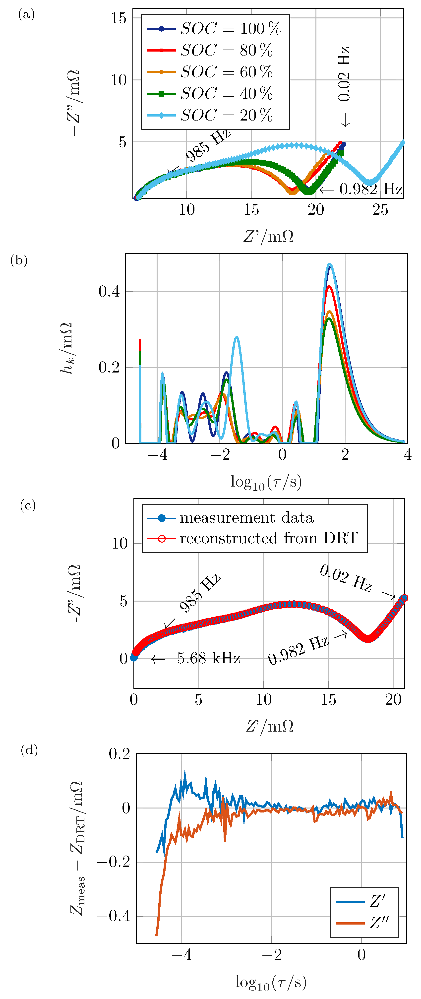
4. Analysis of Measurement Data

The algorithm was applied on measured impedance spectra to validate the method and to quantify the predominant polarization effects in a real electrochemical system. As specimen, a commercial Li-ion battery, Kokam SLPB526495 with a nominal capacity of $3.3$ Ah in pouch cell format with a high energy NMC cathode was investigated. The impedance spectrum was measured using a Zahner ZENNIUM pro electrochemical workstation applying galvanostatic EIS at an amplitude of 120 $\mathrm{m}$$\mathrm{A}$ within a frequency range of 20 $\mathrm{m}$$\mathrm{Hz}$ to 5 $\mathrm{k}$$\mathrm{Hz}$ with 21 steps per decade. The $SOC$ (state of charge) was varied between 20% and 100% in 20% steps. For the variation, the cell was charged to 100% $SOC$ as recommended by the manufacturer. After 3 $\mathrm{h}$ of relaxation, the impedance was measured. Then, the cell was repeatedly discharged at 0.5C for $\Delta SOC=20\%$. Again, after 3 $\mathrm{h}$ of relaxation, the impedance was measured. The five resulting spectra are displayed in Figure 7a. The upper frequency limit was set so that there was no inductive behavior within the spectrum, while interface processes and the diffusion branch were visible. The ohmic resistance increased monotonously from $5.9$ $\mathrm{m}$$\Omega$ to $6.1$ $\mathrm{m}$$\Omega$ with decreasing $SOC$. The high-frequency feature of the impedance spectrum is typically associated with the process at the current collector/active material interface process [4]. Though, this assignment has to be studied carefully as there might be inductive contributions within that frequency range. The mid-frequency feature was strongly dependent on the $SOC$. It can be assumed that the underlying process was related to the charge transfer reaction [4]. The diffusion, which occurs at low frequencies, did not seem to show an obvious $SOC$-dependency within the Nyquist plot. A quantitative comparison is hard due to the offset in Re(Z) and possibly overlapping electrode processes between the different graphs.

In Figure 7b, the distribution functions of the spectra in Figure 7a are shown. The DRT have been obtained by applying the cut-and-shift approach introduced in Section 2. In addition, the range of time constants has been extended by three decades towards low frequencies compared to the measured range also introduced within Section 2. The branch itself was fitted to the time constants for the measured frequencies, while semi-circles which were caused by contributions of lower frequencies in $h_k$ are necessary to bypass the resistive–capacitive restriction. This procedure was proven to be suitable by comparing the reconstructed spectrum to the original data in Figure 7c as the graphs do not deviate strongly at 20% $SOC$. The reconstructions of the other $SOC$s have been of equal quality (not shown here). Only for high frequencies, the graphs do not entirely match due to the onset of superimposed inductive contributions. This influence must be neglected for the DRT anyway. For the data point at 20 $\mathrm{m}$$\mathrm{Hz}$ there was a deviation due to the non-RC restriction which cannot be compensated perfectly, but in a sufficient manner.

Figure 7d shows the absolute residual between measured and reconstructed impedance within the measured frequency range where $Z^{″}>0$. Due to the cut-and-shift approach, the data point for the highest displayed frequency is close to zero. Thus, even a small difference would lead to a huge relative error which, in this case, is of no specific relevance. The good quality of the fit is proven by deviations below $0.2$$\mathrm{m}$$\Omega$ for the entire spectrum, except the very small time constants. As stated above, this was caused by a beginning inductive influence, which can neither be avoided nor subtracted precisely. For the highest time constants, the difference begins to grow as the limitations regarding Equation (5) begin to impact the reconstructed spectrum.

Analyzing Figure 7b in more detail, the absolute distribution function h is used instead of g, enabling both a quantitative and qualitative analysis as the distribution functions are all within the same magnitude. The value $h_1$, representing the contribution of the lowest time constant, is not equal to zero. This is caused by a combination of imperfect subtraction of the purely ohmic resistance and the presence of some minor inductive contributions at high frequencies. The absolute value of $h_1$ is strongly dependent on the number of measurement points, the regularization parameter and the number of time constants used within the DRT. This peak can be ignored for further investigations as it is not related to an electrode process. At high time constants, the contribution of the solid-state diffusion is dominant. Preliminary studies with constant phase and Warburg elements have shown that the three peaks closest to the main peak are also diffusion-related and necessary for a precise reconstruction. This is in accordance to a recent publication by Boukamp [38] who also derives a formula for the characteristic time constants of the peaks obtained in relation to the exact time constant calculated from finite length Warburg element formula. The results of our preliminary study are in very good accordance to the formula given as [38]

$$\begin{array}{c}\hfill {\tau }_i=\frac{{\tau }_0}{{\pi }^2·{(i-0.5)}^2},\end{array}$$

(22)

where the main diffusion peak is referred to as ${\tau }_1$ and the smaller ones as ${\tau }_2$, ${\tau }_3$ etc. with decreasing time constant, respectively. With synthetic Warburg data, ${\tau }_0$ calculated from ${\tau }_1$ to ${\tau }_3$ is equal. Increasing the regularization parameter, the calculated ${\tau }_0$ differ increasingly, especially for high indices of $\tau$, and shift towards lower time constants. Investigating the battery as a whole, the match of the theoretical and practical peak positions ${\tau }_0$ differs up to a factor of eight between the three small and one large diffusion-related peaks. Furthermore, at 60% there is a small additional peak visible. This non-ideal behavior may be caused by the distributed solid-phase diffusion throughout the porous electrode material and by the simultaneous presence of anode and cathode diffusion process. These result in non-ideal Warburg behavior in combination with the regularization-based effect as mentioned above. Further, the polarization resistances of the four peaks differ from their theoretical values for the same reason.

In contrast to Figure 7a, a significant change in diffusive behavior becomes visible when investigating the DRT. For intermediate $SOC$s, the diffusion shows a smaller peak in the DRT than for high or low $SOC$s within the measured frequency range. As previously seen in Figure 7a, the slowest interface process is strongly dependent on the electrodes’ $SOC$ and therefore on the lithium surface concentration of the particles. Starting with the fully charged cell, the polarization and the characteristic time constant decreases strongly and is almost constant for 80% and 60%. When discharging further, the polarization rises by more than a factor of two and the time constant shifts towards higher values. At around $\tau \approx$ 1 × 10${}^{-3}$ s there are two more processes visible. Due to their characteristic time constants, it can be assumed that these peaks represent electrode or interface processes. The faster process shows the highest polarization resistance at 20% and 100%, while the value is lower and close to constant for intermediate SOCs. The fastest process shows a constant shape and height. For further investigations, a quantitative analysis of the three electrode process-related peaks is inevitable.

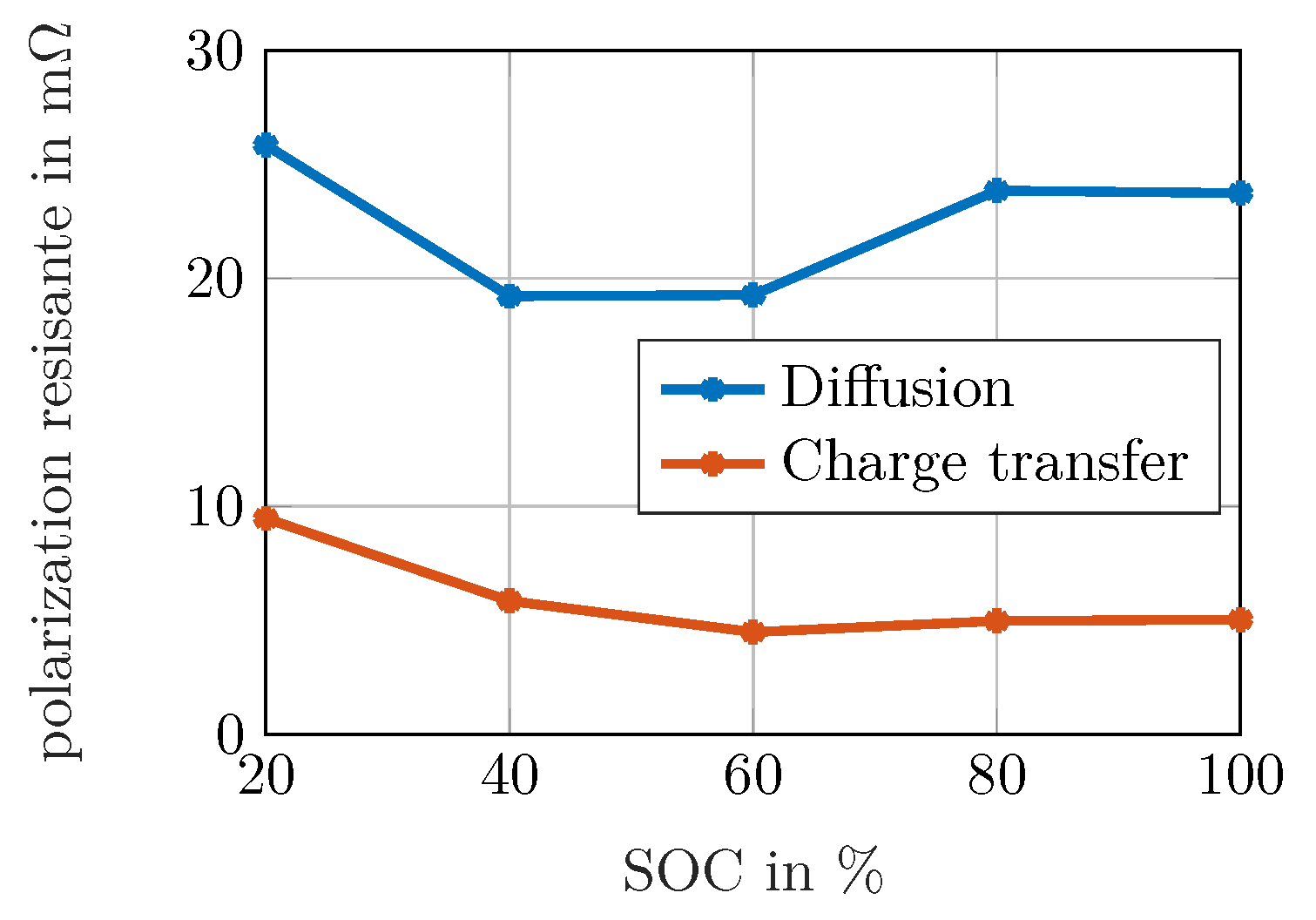
The peak analysis shown in Figure 8 allows a quantitative analysis of each separate distribution in Figure 7b. As mentioned above, peak 1 does not show a noteworthy SOC-dependency and has a polarization resistance of $1.8$ $\mathrm{m}$$\Omega$. It can be assumed that this peak represents the particle-particle or particle-current collector interface [4].

Peaks 2 and 4 show a similar SOC dependency: For high and low SOCs, the polarization resistance is large, while it is low for intermediate SOCs. The higher the resistance, the higher is furthermore the time constant. The width of the peaks does only change due to the change in height. As there are two charge transfer reactions expected within the battery, it can be assumed that peaks 2 and 4 represent those. Peak 3 behaves differently: it significantly changes its width and the characteristic time constant at 60% is lower than could be expected when compared to the other SOCs. This peak could hence be assigned to the SEI, while the exact reason for this behavior remains unclear. Considering these findings, peak 4 can be assigned to the anodic charge transfer reaction based on the following indicators:

• The time constant of the anodic charge transfer is typically higher than that of the SEI [39,40]
• The resistance increases for high and low values reaching a minimum at medium $SOC$s. Figure 9 underlines this observation. This is in accordance with the Butler–Volmer kinetics, where the exchange current density is small at high and low $SOC$s [14,41]. To differentiate the process from the cathodic reaction, Figure 9 shows that the resistance is highest at low SOCs, whereas the increase is only shallow at 80% and 100%. It has to be considered that in commercial cells, the anode is over-dimensioned so that lithium plating is avoided by restricting high lithium concentrations in the anode. This leads to an disproportionate distribution of the anode’s degree of lithiation. Thus, its SOC is not well-proportionate but shifted towards smaller concentrations. This leads to the conclusion that peak 3 is caused by the anodic charge transfer reaction.

The qualitative investigation of the diffusive process in Figure 9 is of interest as well. The absolute value is calculated by adding the resistances of peaks 5–8. Summing up the values of charge transfer and diffusion obtained e.g., for 20% $SOC$, approx. 37 $\mathrm{m}$$\Omega$ are achieved. However, the maximum value of $\left|Z\right|$ is below 30 $\mathrm{m}$$\Omega$ in Figure 7a. As the assumption of convergence towards $Im\left(Z\left(j{\omega }_{\min }\right)\right)=0$ for frequencies below the measured range is not necessarily fulfilled, e.g., when a limited reservoir leads to capacitive behavior for very low frequencies, the polarization contribution obtained for the diffusive branch must neither be interpreted as an absolute value for an overall diffusion resistance nor be used to draw conclusions of processes outside the measured frequency range. Instead, the values can be taken into account for a comparison of different spectra to visualize changes in diffusive behavior, if the frequency range and the regularization parameter is equal for the investigated spectra.

The qualitative behavior of the diffusive values can be interpreted in two ways: in a descriptive manner, the diffusion is limited when the concentrations are either close to the maximum while there are still more ions to be intercalated and transported towards the particles’ center or when the concentration is close to zero, but there is a demand of ions from the inner particle to be deintercalated at the surface. Considering electrochemistry, diffusion leads to a high polarization when the differential capacity is small, i.e., a small change of concentration leads to a large change in the open circuit voltage when the surface concentration differs from the average concentration. This is the case at high SOCs, but even stronger at low SOCs for the investigated NMC cell. Both explanations lead to the same result: As the resistance increases for high and for low SOCs in a similar way, it can be assumed that anodic and cathodic solid state diffusion overlap within the diffusion peak showing similar time constants without the possibility of separation.

Analyzing the DRT, we are able to gain significantly more information on the dominant polarization mechanisms. The $SOC$ dependency of solid state diffusion could be assessed quantitatively and the dominating electrode processes could be assigned to peak 2–4.

5. Conclusions

The DRT offers a model-free characterization for electrochemical systems. Its information value is strongly dependent on a proper choice of process parameters which are needed to solve the ill-posed problem. Choosing the regularization parameter $\lambda$ too small leads to oscillations and a large number of peaks not connected to physical processes. A large regularization parameter leads to a merger of peaks so that independent processes cannot be separated properly. In our case, $\lambda$ should be chosen between 0.1 and 0.2. This value is strongly dependent on the exact algorithm used as there are publications using $\lambda$ differing by magnitudes. The measurement data and its signal-to-noise-ratio also influences the optimum value. The number of sampling points of time constants for the DRT analysis should be large enough for a smooth result. Exceeding a reasonable amount increases the computational effort without significant improvements to the result, though. The threefold number of measured frequency points has shown to be appropriate. A smaller number increases the difference between measured and reconstructed impedance spectrum notably, while a higher number does not reduce the error significantly. Choosing the highest time constant three decades above the minimum measured frequency, processes where $\underset{\tau \to 0}{lim}(\mathrm{Im}\left(Z\right))\ne 0$ can be analyzed.

The regularization parameter can be used as a linear factor on the distribution function itself or on the first or second derivative. Dependent on that, either the absolute height, the slope or the curvature is regularized leading to contrasting effects on $g_k$. The implementation of those approaches verifies this hypothesis. We recommend to use the non-derived regularization matrix for most cases. Furthermore, the optimization algorithm used, the optimization function fed into the algorithm and the way the algorithm deals with the non-negativity constraint affect the outcome. This constraint is physically inevitable as there must not be negative contributions to the overall polarization. With the parameters set as above, processes with similar polarization resistances can be separated if their time constants differ by a factor of two to four. The exact factor cannot be determined in advance but is dependent on the shape of the individual peaks. If the polarization resistance of peaks differ strongly, the gap between the characteristic time constants needs to be higher to be able to observe the smaller peak. The algorithm used is available at http://www.ec-idea.uni-bayreuth.de within a software package based on the Matlab runtime environment.

The introduced peak analysis algorithm facilitates the separation of the peaks and enables the calculation of the individual polarization resistances. One large and several smaller peaks at high time constants can be assigned to solid state diffusion. A hypothesis was established to correlate three specific peaks to the anodic and cathodic charge transfer and the SEI due to their time constants and SOC behavior. For both identified processes, diffusion and charge transfer, a non-monotonous behavior emerges with a maximum polarization resistance for low SOCs, decreasing for medium and again increasing resistances for high SOCs. Investigating the impedance spectrum only, e.g., by fitting equivalent circuits, there is no evidence on the number of involved processes. The DRT offers the benefit of a detailed insight into the electrochemical mechanisms taking place in the specimen and their characteristic time constants.

References

1. Ivers-Tiffée, E.; Weber, A. Evaluation of electrochemical impedance spectra by the distribution of relaxation times. J. Ceram. Soc. Jpn. 2017, 125, 193–201. [Google Scholar] [CrossRef] [Green Version]
2. Illig, J.; Schmidt, J.P.; Weiss, M.; Weber, A.; Ivers-Tiffée, E. Understanding the impedance spectrum of 18650 LiFePO4-cells. J. Power Sources 2013, 239, 670–679. [Google Scholar] [CrossRef]
3. Barsoukov, E. Kinetics of lithium intercalation into carbon anodes: In situ impedance investigation of thickness and potential dependence. Solid State Ionics 1999, 116, 249–261. [Google Scholar] [CrossRef]
4. Illig, J.; Ender, M.; Weber, A.; Ivers-Tiffée, E. Modeling graphite anodes with serial and transmission line models. J. Power Sources 2015, 282, 335–347. [Google Scholar] [CrossRef]
5. Costard, J.; Ender, M.; Weiss, M.; Ivers-Tiffée, E. Three-Electrode Setups for Lithium-Ion Batteries: II. Experimental Study of Different Reference Electrode Designs and Their Implications for Half-Cell Impedance Spectra. J. Electrochem. Soc. 2016, 164, A80–A87. [Google Scholar] [CrossRef]
6. Graves, C.; Ebbesen, S.D.; Mogensen, M. Co-electrolysis of CO2 and H2O in solid oxide cells: Performance and durability. Solid State Ionics 2011, 192, 398–403. [Google Scholar] [CrossRef]
7. Weiß, A.; Schindler, S.; Galbiati, S.; Danzer, M.A.; Zeis, R. Distribution of Relaxation Times Analysis of High-Temperature PEM Fuel Cell Impedance Spectra. Electrochim. Acta 2017, 230, 391–398. [Google Scholar] [CrossRef]
8. Hanft, D.; Exner, J.; Moos, R. Thick-films of garnet-type lithium ion conductor prepared by the Aerosol Deposition Method: The role of morphology and annealing treatment on the ionic conductivity. J. Power Sources 2017, 361, 61–69. [Google Scholar] [CrossRef]
9. Exner, J.; Fuierer, P.; Moos, R. Aerosol deposition of (Cu,Ti) substituted bismuth vanadate films. Thin Solid Film. 2014, 573, 185–190. [Google Scholar] [CrossRef]
10. Thomas, B.J.; Ward, L.C.; Cornish, B.H. Bioimpedance spectrometry in the determination of body water compartments: Accuracy and clinical significance. Appl. Radiat. Isot. 1998, 49, 447–455. [Google Scholar] [CrossRef]
11. Schindler, S.; Danzer, M.A. Influence of cell design on impedance characteristics of cylindrical lithium-ion cells: A model-based assessment from electrode to cell level. J. Energy Storage 2017, 12, 157–166. [Google Scholar] [CrossRef]
12. Schönleber, M.; Uhlmann, C.; Braun, P.; Weber, A.; Ivers-Tiffée, E. A Consistent Derivation of the Impedance of a Lithium-Ion Battery Electrode and its Dependency on the State-of-Charge. Electrochim. Acta 2017, 243, 250–259. [Google Scholar] [CrossRef]
13. Schindler, S.; Bauer, M.; Petzl, M.; Danzer, M.A. Voltage relaxation and impedance spectroscopy as in-operando methods for the detection of lithium plating on graphitic anodes in commercial lithium-ion cells. J. Power Sources 2016, 304, 170–180. [Google Scholar] [CrossRef]
14. Kindermann, F.M.; Noel, A.; Erhard, S.V.; Jossen, A. Long-term equalization effects in Li-ion batteries due to local state of charge inhomogeneities and their impact on impedance measurements. Electrochim. Acta 2015, 185, 107–116. [Google Scholar] [CrossRef]
15. Schichlein, H.; Müller, A.C.; Voigts, M.; Krügel, A.; Ivers-Tiffée, E. Deconvolution of electrochemical impedance spectra for the identification of electrode reaction mechanisms in solid oxide fuel cells. J. Appl. Electrochem. 2002, 32, 875–882. [Google Scholar] [CrossRef]
16. Sumi, H.; Yamaguchi, T.; Hamamoto, K.; Suzuki, T.; Fujishiro, Y.; Matsui, T.; Eguchi, K. AC impedance characteristics for anode-supported microtubular solid oxide fuel cells. Electrochim. Acta 2012, 67, 159–165. [Google Scholar] [CrossRef]
17. Schmidt, J.P.; Berg, P.; Schönleber, M.; Weber, A.; Ivers-Tiffée, E. The distribution of relaxation times as basis for generalized time-domain models for Li-ion batteries. J. Power Sources 2013, 221, 70–77. [Google Scholar] [CrossRef]
18. Boukamp, B.A. A Linear Kronig-Kramers Transform Test for Immittance Data Validation. J. Electrochem. Soc. 1995, 142, 1885. [Google Scholar] [CrossRef] [Green Version]
19. Schönleber, M.; Klotz, D.; Ivers-Tiffée, E. A Method for Improving the Robustness of linear Kramers-Kronig Validity Tests. Electrochim. Acta 2014, 131, 20–27. [Google Scholar] [CrossRef]
20. Sonn, V.; Leonide, A.; Ivers-Tiffée, E. Combined Deconvolution and CNLS Fitting Approach Applied on the Impedance Response of Technical Ni/8YSZ Cermet Electrodes. J. Electrochem. Soc. 2008, 155, B675. [Google Scholar] [CrossRef]
21. Tröltzsch, U.; Kanoun, O.; Tränkler, H.R. Characterizing aging effects of lithium ion batteries by impedance spectroscopy. Electrochim. Acta 2006, 51, 1664–1672. [Google Scholar] [CrossRef]
22. Nara, H.; Mukoyama, D.; Yokoshima, T.; Momma, T.; Osaka, T. Impedance Analysis with Transmission Line Model for Reaction Distribution in a Pouch Type Lithium-Ion Battery by Using Micro Reference Electrode. J. Electrochem. Soc. 2015, 163, A434–A441. [Google Scholar] [CrossRef] [Green Version]
23. Tikhonov, A.N. Numerical Methods for the Solution of Ill-Posed Problems; Springer: Dordrecht, The Netherlands, 2010. [Google Scholar]
24. Weese, J. A reliable and fast method for the solution of Fredholm integral equations of the first kind based on Tikhonov regularization. Comput. Phys. Commun. 1992, 69, 99–111. [Google Scholar] [CrossRef]
25. Ciucci, F.; Chen, C. Analysis of Electrochemical Impedance Spectroscopy Data Using the Distribution of Relaxation Times: A Bayesian and Hierarchical Bayesian Approach. Electrochim. Acta 2015, 167, 439–454. [Google Scholar] [CrossRef]
26. Wan, T.H.; Saccoccio, M.; Chen, C.; Ciucci, F. Influence of the Discretization Methods on the Distribution of Relaxation Times Deconvolution: Implementing Radial Basis Functions with DRTtools. Electrochim. Acta 2015, 184, 483–499. [Google Scholar] [CrossRef]
27. de L. Kronig, R. On the Theory of Dispersion of X-rays. J. Opt. Soc. Am. 1926, 12, 547. [Google Scholar] [CrossRef]
28. Kramers, M.H.A. La diffusion de la lumière par les atomes. Trans. Volta Centenary Congr. 1927, 2, 545–557. [Google Scholar]
29. Lawson, C.L.; Hanson, R.J. Solving least squares problems. In Classics in Applied Mathematics; Society for Industrial and Applied Mathematics: Philadelphia, PA, USA, 1995; Volume 15. [Google Scholar]
30. Kaipio, J.; Somersalo, E. Statistical and computational inverse problems. In Applied Mathematical Sciences; Springer: New York, NY, USA, 2010; Volume 160. [Google Scholar]
31. Wu, L. A Parameter Choice Method for Tikhonov Regularization. Electron. Trans. Numer. Anal. 2003, 16, 107–128. [Google Scholar]
32. Gavrilyuk, A.L.; Osinkin, D.A.; Bronin, D.I. The use of Tikhonov regularization method for calculating the distribution function of relaxation times in impedance spectroscopy. Russ. J. Electrochem. 2017, 53, 575–588. [Google Scholar] [CrossRef]
33. Davies, A.R.; Anderssen, R.S. Optimisation in the regularisation ill-posed problems. J. Aust. Math. Soc. Ser. B Appl. Math. 1986, 28, 114. [Google Scholar] [CrossRef] [Green Version]
34. Saccoccio, M.; Wan, T.H.; Chen, C.; Ciucci, F. Optimal Regularization in Distribution of Relaxation Times applied to Electrochemical Impedance Spectroscopy: Ridge and Lasso Regression Methods—A Theoretical and Experimental Study. Electrochim. Acta 2014, 147, 470–482. [Google Scholar] [CrossRef]
35. Hansen, P.C. Analysis of Discrete Ill-Posed Problems by Means of the L-Curve. SIAM Rev. 1992, 34, 561–580. [Google Scholar] [CrossRef]
36. Hansen, P.C.; O’Leary, D.P. The Use of the L-Curve in the Regularization of Discrete Ill-Posed Problems. SIAM J. Sci. Comput. 1993, 14, 1487–1503. [Google Scholar] [CrossRef] [Green Version]
37. Byrd, R.H.; Gilbert, J.C.; Nocedal, J. A trust region method based on interior point techniques for nonlinear programming. Math. Program. 2000, 89, 149–185. [Google Scholar] [CrossRef] [Green Version]
38. Boukamp, B.A. Derivation of a Distribution Function of Relaxation Times for the (fractal) Finite Length Warburg. Electrochim. Acta 2017, 252, 154–163. [Google Scholar] [CrossRef]
39. Levi, M.D.; Aurbach, D. Simultaneous Measurements and Modeling of the Electrochemical Impedance and the Cyclic Voltammetric Characteristics of Graphite Electrodes Doped with Lithium. J. Phys. Chem. B 1997, 101, 4630–4640. [Google Scholar] [CrossRef]
40. Piao, T. Intercalation of Lithium Ions into Graphite Electrodes Studied by AC Impedance Measurements. J. Electrochem. Soc. 1999, 146, 2794. [Google Scholar] [CrossRef] [Green Version]
41. Fuller, T.F. Simulation and Optimization of the Dual Lithium Ion Insertion Cell. J. Electrochem. Soc. 1994, 141, 1. [Google Scholar] [CrossRef] [Green Version]
Figure 1. Impedance spectrum of two RC elements connected in series (a) appearing as a single, asymmetric semi-circle in the Nyquist plot; the distribution of relaxation times (DRT) (b) reveals both processes involved.
Batteries 05 00043 g001
Figure 2. Flowchart of DRT algorithm for handling real, non-ideal measurement data.
Batteries 05 00043 g002
Figure 3. DRT of an RC-element ( R 1 = 5   m Ω , C 1 = 0 , 1   F ) and a ZARC-element ( R 2 = 7   m Ω , C 2 = 0 , 71   F , φ = 0.8 ) in series, calculated at five different λ logarithmically equally-distributed between 0.001 and 10.
Batteries 05 00043 g003
Figure 4. The sum of squared errors ( s s e ) of the reconstructed spectra for differing n and a variation of λ between 0.01. and 2 (a) and a magnified detail for small λ (b), g k for λ = 0.1 and varied n (c) and c · g k (d), where c is the multiple of m for every line respectively.
Batteries 05 00043 g004
Figure 5. Condition number of the regularized matrix A for 100 to 500 time constants between 10 m Hz and 10 k Hz and λ from Figure 3. Condition number for non-regularized matrix between 1.1 × 10 19 and 8.2 × 10 19 .
Batteries 05 00043 g005
Figure 6. (a) DRT of an RC- ( R 1 = 5   m Ω , C 1 = 0 , 1   F ) and a ZARC-element ( R 2 = 7   m Ω , C 2 = 0 , 71   F , φ = 0.8 ) in series, λ = 0.1 , n = 3 m . Algorithm 1 as pointed out within Section 2, Algorithm 2 using an interior-point method, (b) using identity matrix, first and second derivative for regularization. (c) Showing the regularization term representing the matrix according to (b).
Batteries 05 00043 g006
Figure 7. (a) Measured impedance spectra of commercial High Energy-NMC cell at varied S O C s (frequencies correspond to 100% S O C , (b) non-normalized distribution of time constants, (c) measured and reconstructed impedance spectrum for 20% S O C , (d) absolute residual between measured and reconstructed impedance for 20% S O C .
Batteries 05 00043 g007
Figure 8. Non-normalized DRT with peak analysis for (a) 100% S O C , (b) 80% S O C , (c) 60% S O C , (d) 40% S O C , (e) 20% S O C .
Batteries 05 00043 g008
Figure 9. Polarization resistance of (presumably anodic) charge transfer (peak 4) reaction and the value obtained by the DRT for the diffusion of both electrodes (which must not be interpreted as an absolute resistance value).
Batteries 05 00043 g009