Abstract
Large-scale battery datasets often contain anomalous data due to sensor noise, communication errors, and operational inconsistencies, which degrade the accuracy of data-driven prognostics. However, many existing studies overlook the impact of such anomalies or apply filtering heuristically without rigorous benchmarking, which can potentially introduce biases into training and evaluation pipelines. This study presents a deep learning framework that integrates autoencoder-based anomaly detection with a residual neural network (ResNet) to achieve state-of-the-art prediction of remaining useful life at the cycle level using only a single-cycle input. The framework systematically filters out anomalous samples using multiple variants of convolutional and sequence-to-sequence autoencoders, thereby enhancing data integrity before optimizing and training the ResNet-based models. Benchmarking against existing deep learning approaches demonstrates a significant performance improvement, with the best model achieving a mean absolute percentage error of 2.85% and a root mean square error of 40.87 cycles, surpassing prior studies. These results indicate that autoencoder-based anomaly filtering significantly enhances prediction accuracy, reinforcing the importance of systematic anomaly detection in battery prognostics. The proposed method provides a scalable and interpretable solution for intelligent battery management in electric vehicles and energy storage systems.
1. Introduction
As global adoption of electric vehicles (EVs) continues to accelerate, precise prediction of the remaining useful life (RUL) of lithium-ion batteries has become increasingly critical for optimizing maintenance schedules, mitigating operational risks, and ensuring vehicle safety and operational efficiency. Recent advancements in cloud-based data acquisition capabilities have enabled the extensive collection and real-time transmission of operational data from lithium-ion battery systems in EVs and energy storage systems (ESS) [1,2]. However, such large-scale datasets commonly include anomalous or unqualified samples attributable to measurement inconsistencies, communication errors and noise, complicating accurate battery prognostics [3]. Consequently, developing robust methodologies to effectively manage and mitigate the influence of anomalous data remains one of the challenges in battery prognostics. Additionally, recent studies have introduced novel methodologies, such as Chen et al.’s impedance estimation using support vector regression optimized by a cuckoo search algorithm [4] and Li et al.’s hybrid neural network employing feature fusion and transfer learning strategies for improved battery state-of-health (SOH) estimation [5].
Autoencoder-based methods have emerged as powerful tools for anomaly filtering, data generation, and robust feature representation. Depending on their structure and training objectives, these models can be broadly categorized into five architectural types: standard autoencoders (AE), denoising autoencoders (DAE), variational autoencoders (VAE), conditional variational autoencoders (CVAE), and adversarial autoencoders (AAE).
Standard autoencoders typically reduce dimensionality or transform features for predictive tasks [6,7]. DAEs are effective in handling sensor noise and missing data, enhancing robustness in real-world battery prognostics [8,9,10]. VAEs model uncertainty, generate synthetic data, and detect anomalies through reconstruction errors and probabilistic distributions [11,12,13,14]. CVAEs utilize supervised signals to guide generative modeling and improve predictive accuracy [15,16]. AAEs enforce feature realism and domain invariance, further improving generalization [14,17,18]. While various autoencoder architectures have been explored, direct comparisons remain challenging due to limited datasets with explicit failure annotations. Therefore, their effectiveness is often indirectly assessed by their contributions to performance improvements in downstream tasks, such as RUL or SOH prediction, after anomaly filtering [6,8,9,16,19,20].
Another crucial factor affecting deep learning-based prediction is the scale of the training and validation datasets. As Iglesia et al. [21] highlight in their systematic review, dataset size is crucial for ensuring robust model generalization. Models trained on relatively small datasets risk overfitting to dataset-specific degradation patterns, thereby reducing their applicability across diverse real-world conditions. In this study, we utilize the largest publicly available lithium-ion battery dataset from Stanford-MIT [22], which comprises 124 battery cells. Although this dataset has been criticized for its near-constant discharge conditions [23], it encompasses 72 distinct charging policies, offering a variety of operational patterns. This diversity helps mitigate concerns of overfitting and provides a more comprehensive basis for developing and evaluating deep learning models in battery RUL prediction.
Hsu et al. [24] reported significant advancements in predicting RUL using DNNs, achieving notably low prediction errors with a mean absolute percentage error (MAPE) below 4% and a root mean square error (RMSE) of fewer than 50 cycles using only a single cycle of input data. This demonstrates substantial potential for high-accuracy, early-life battery prognostics leveraging DNN architectures. However, a critical examination of their data selection and filtering methodology reveals important areas that need clarification and standardization. Although the authors excluded battery samples based on experimental issues such as early test termination, temperature recording failures, and excessive signal noise, explicit quantitative thresholds or statistically supported benchmarks for these exclusions were not defined. Specifically, from the original dataset, only 115 batteries had discharge data deemed sufficient within the initial 100 cycles for the Discharge DNN. Further selection reduced this to 95 batteries with acceptable charging data, and eventually to 81 batteries possessing consistently high-quality discharge and charge data for use in their Full RUL DNN.
Despite detailing reasons for these exclusions, the authors did not provide quantitative standards or statistical validation to ensure the absence of potential biases. Clearly defined standards would enhance the reliability of the findings and help differentiate model innovation from improvements that may result from selective data omission or biases. Furthermore, a systematic machine-learning approach can reveal patterns and enable discoveries that surpass human intuition and traditional methods [25].
Several studies have employed the MIT dataset for early-stage RUL prediction as shown in Table 1. Tang et al. [26] used a CNN-LSTM model with early incremental capacity (IC) curves, achieving 146 RMSE and 13.4% MAPE using 100 cycles. Couture and Lin [27] combined health indicators with CNN-based image features and a fully connected neural network (FCNN), reporting 79.7 RMSE and 11.2% MAPE using 10 cycles from 94 filtered cells. Safavi et al. [28] applied a CNN-XGBoost model on all 124 cells, reaching 106 RMSE and 7.5% MAPE. Gong et al. [29] used evolutionary feature selection (FS), neighborhood component analysis (NCA), and differential evolution (DE) combined with XGBoost/relevance vector machine (RVM), obtaining 43 RMSE and 5.21% MAPE. Fei et al. [30] employed CNN (VGG-16) with gaussian process regression (GPR), achieving 112 RMSE and 8.2% MAPE. Sanz-Gorrachategui et al. [31] used adversarial CNNs with leave-one-out cross-validation (CV), reporting 62 RMSE and 5% MAPE. Yang et al. [32] and Zhang et al. [33] proposed hybrid CNN models that integrate 2D/3D convolutions and attention mechanisms, achieving state-of-the-art performance with as few as 10–60 cycles across all 124 cells. Zhang et al. [33] specifically utilized a hybrid parallel residual (HPR)-CNN architecture.

Table 1.
Comparative summary of machine learning methods for battery RUL prediction.
This study proposes a robust ResNet-based deep learning framework integrated with autoencoder-driven anomaly detection to significantly advance battery RUL prediction. By systematically filtering anomalous data, this approach effectively reduces bias and enhances model generalization. A key novelty of this work lies in comprehensively comparing multiple autoencoder architectures to determine their effectiveness in anomaly detection, highlighting how the choice of architecture directly impacts RUL prediction performance. Extensive hyperparameter optimization of both autoencoder models and the ResNet architecture underscores the rigorous and innovative nature of this experimental effort. Given the practical difficulty of acquiring explicitly labeled faulty battery data, autoencoders offer a scalable, unsupervised approach for anomaly detection [35]. The proposed framework achieves state-of-the-art RUL prediction accuracy (MAPE 2.85%, RMSE 40.87 cycles) using only single-cycle battery data. Furthermore, interpretability is enhanced through detailed feature importance analysis using SHAP and tree-based methods, providing a transparent and comparative methodology for anomaly filtering and significantly improving downstream predictive performance.
2. Method
2.1. Overall Framework
The overall framework of this study, illustrated in Figure 1, comprises multiple systematic procedures designed to ensure robust and accurate prediction of RUL. Initially, interpolation techniques are applied to standardize all battery cycle data, resulting in a consistent representation of 1000 data points per cycle. Subsequent feature selection is carefully guided by criteria that ensure independence across battery cycles, explicitly excluding statistical features that vary across cycles. Instead, the study utilizes raw measurements directly obtainable from practical battery management systems (BMS), including voltage, current, temperature, and integrated capacity during both charging and discharging phases for training autoencoders. K-fold cross-validation is implemented to thoroughly assess the generalization and predictive performance of the proposed models. This validation procedure partitions the dataset into three subsets, iteratively utilizing each subset for validation while training with the remaining subsets. Furthermore, autoencoders detect and remove anomalous data samples based on reconstruction error criteria. Consequently, 25 out of the initial 124 cells are excluded, leaving a dataset comprising 99 cells for subsequent analysis. Even after this filtering step, the remaining dataset size surpasses that utilized in previously published benchmark studies, notably the single-cycle RUL prediction approach by Hsu et al. [24]. Finally, hyperparameter optimization of the ResNet architecture is conducted through a systematic grid search approach.
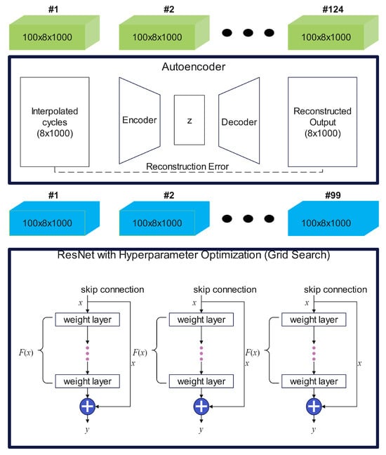
Figure 1.
Overall framework of the proposed methodology for lithium-ion battery RUL prediction. The workflow comprises two primary stages. First, raw battery cycle data (green, dimensions: 100 cycles × 8 features × 1000 time steps per cycle) are interpolated and processed by autoencoder architectures for systematic anomaly filtering based on reconstruction error. The eight sequential input features per cycle include voltage, current, temperature, integrated charge capacity (QC), integrated discharge capacity (QD), linearly interpolated discharge capacity (QDlin), linearly interpolated temperature (Tdlin), and internal resistance (IR). The autoencoder identifies anomalous cycles, filtering them out to yield a refined dataset (blue). The refined dataset is subsequently used as input to the ResNet model, optimized through hyperparameter tuning (grid search), specifically adjusting kernel size and incorporating batch normalization layers. The ResNet inputs consist of 14 statistical features per battery cycle: average voltage, maximum voltage, minimum voltage, average temperature, maximum temperature, minimum temperature, integrated charge capacity (QC), integrated discharge capacity (QD), linearly interpolated discharge capacity (QDlin), linearly interpolated temperature (Tdlin), internal resistance (IR), average incremental capacity (dQ/dV), maximum incremental capacity (dQ/dV), and minimum incremental capacity (dQ/dV). The final ResNet model outputs cycle-level RUL predictions for each battery cell.
2.2. Autoencoders
Convolutional autoencoder(CAE) and sequence-to-sequence (Seq2Seq) architectures in Appendix A are developed to systematically identify and remove anomalous or inconsistent battery cycle data based on reconstruction errors. Each CAE variant employs 1D-CNNs, using specialized dimensionality reduction strategies tailored to either raw sequential battery data or statistical features summarizing each cycle. The Seq2Seq autoencoder variants utilize LSTM units, which explicitly capture sequential dependencies within battery cycle data. Autoencoder models are designed to learn latent representations of input data and reconstruct the original input with minimal error.
The transformation of input data through a CAE follows a hierarchical feature extraction process, where each layer refines the representation of the previous one. Mathematically, the latent representation at a given layer is expressed as:
where denotes the latent feature representation at layer l, and correspond to the convolutional filter weights and biases, respectively, and ∗ represents the convolution operation. The activation function introduces nonlinearity to enable complex feature extraction. The reconstructed output is obtained by applying a transposed convolution to the final latent representation:
where represents the final encoded feature representation, and and are learnable parameters of the decoder. This structure enables CAEs to learn spatially meaningful latent features, which is advantageous in applications such as anomaly detection and feature compression.
In contrast, the Seq2Seq autoencoder employs RNNs to capture temporal dependencies in sequential data. The encoding process utilizes an LSTM network to transform an input sequence into a fixed-dimensional latent representation:
where denotes the input vector at time step t and is the encoder LSTM’s hidden state at time t. The final hidden state of the encoder serves as a compressed representation of the entire input sequence. This encoded representation is then fed into a decoder LSTM, which sequentially reconstructs the original input:
Here, is the decoder’s hidden state at time t, is the reconstructed output from the previous time step, and represents a transformation function that maps the decoder’s hidden state to the output space. This Seq2Seq structure effectively learns temporal dependencies, enabling sequence-level reconstructions.
Both CAE and Seq2Seq autoencoders are typically trained by minimizing the reconstruction loss, which is commonly measured using the mean squared error (MSE):
where N represents the number of samples, and and denote the original and reconstructed inputs, respectively. The objective of training is to optimize the model parameters such that the reconstructed output closely matches the input, thereby ensuring an accurate and meaningful representation of the data in the latent space.
The convolutional autoencoder with average pooling (CAE-AvgPool) employs one-dimensional convolutional layers combined with average pooling operations to reduce temporal dimensionality while preserving smooth and stable patterns in battery behavior. In contrast, the convolutional autoencoder with max pooling (CAE-MaxPool) uses max pooling layers that retain only the strongest activations at each pooling step, thereby enhancing sensitivity to transient anomalies or abrupt variations in the battery signal. The deep convolutional autoencoder (CAE-Deep) consists of multiple convolutional layers with progressively decreasing channel dimensions, allowing it to capture hierarchical temporal dependencies across multiple scales. Its decoder mirrors the encoder using symmetric convolutional and upsampling layers to reconstruct the original input dimensions. Additionally, the convolutional autoencoder with statistical feature extraction (CAE-StatisticalFeature) replaces pooling operations with strided convolutions to compress input features while preserving essential statistical characteristics of the battery cycle data. The decoder reconstructs these representations through convolutional and upsampling layers, concluding with a fully connected output layer matched to the original statistical feature dimensions.
The Simple-Seq2Seq encodes and reconstructs the entire battery sequence using a straightforward single-layer LSTM structure, providing a baseline for temporal modeling performance. The Chunked-Seq2Seq divides input sequences into segments or “chunks”, which are individually processed via TimeDistributed LSTM layers, explicitly modeling localized temporal characteristics within battery data. Reconstruction is performed correspondingly through segmented decoder layers, enhancing local temporal pattern fidelity. The Hierarchical-Seq2Seq incorporates hierarchical LSTM structures to concurrently capture both fine-grained local patterns and overarching global temporal dependencies.
Table 2 presents the averaged training and validation metrics obtained through 3-fold cross-validation for each autoencoder architecture. The variations in reconstruction errors are influenced by factors such as dimensionality reduction strategies, the complexity of input data patterns, and the architecture’s capacity to reconstruct these patterns accurately. For instance, architectures that employ heavily compressed latent representations or model intricate sequential dependencies may exhibit higher reconstruction errors due to the increased difficulty in reconstructing the data. Conversely, autoencoders that process simplified statistical feature inputs often achieve lower reconstruction errors due to the reduced data complexity and dimensionality. It is essential to note that the reconstruction metrics alone are insufficient to directly assess the relative anomaly detection effectiveness of each architecture. A critical evaluation criterion is the ability of the reconstruction error to differentiate between abnormal and normal cells. The Seq2Seq-based autoencoder required approximately 20 s for prediction, whereas the CAE completed predictions in approximately 2 s, indicating that the CAE achieved nearly tenfold faster inference performance. These results were obtained using a dataset comprising 124 samples, each encompassing 100 cycles and 1000 time sequences, conducted on an Intel Core i9-13900KF CPU paired with an NVIDIA GeForce RTX 4090 GPU. It should also be noted that a thorough evaluation of the training durations was not possible due to the variability introduced by the early stopping criteria.
Table 2.
Average training and validation metrics across 3-fold cross-validation for autoencoder architectures.
The training approach employed k-fold cross-validation to objectively evaluate the model’s generalization performance. For convolutional autoencoder (CAE) architectures, models were trained consistently with a fixed batch size of 64 and a learning rate of 0.0001. The training and validation loss curves across multiple folds indicated stable convergence behavior. In the case of the CAE-StatisticalFeature, batch sizes varied from 1 to 32, while the learning rate was constant at 0.001. Experimental results showed a clear trend where increasing batch sizes correlated with enhanced training stability and a statistically significant reduction in reconstruction errors. Similar experimentation was performed for the Seq2Seq autoencoder variants, emphasizing batch size effects. The Simple-Seq2Seq architecture exhibited optimal training performance at a batch size of 128, as evidenced by consistently lower validation errors. Training runs with smaller batch sizes demonstrated inconsistent convergence, higher variability in training outcomes, and reduced reconstruction accuracy.
2.3. Anomaly Detection
Reconstruction errors obtained during model training were analyzed using the 80th percentile approach to determine an anomaly detection threshold. This threshold was specifically selected to ensure a fair comparison with prior studies by controlling the proportion of anomalies identified. Despite filtering anomalies at the 80th percentile, the resulting dataset retained more samples compared to previous research, ensuring robust evaluation. Battery cells exceeding this derived threshold were identified as anomalous in Figure 2. Normal cells are represented in blue, whereas cells identified as anomalous are marked in red. Notably, significant variability in anomaly detection is observed across the autoencoder architectures. For instance, the CAE-AvgPool and CAE-MaxPool models predominantly detect anomalies concentrated within mid-range cell indices, suggesting these architectures’ sensitivity may be limited to specific data patterns or localized anomalies. In contrast, the CAE-Deep, Simple-Seq2Seq, and Chunked-Seq2Seq architectures demonstrate broader, more consistent anomaly detection capabilities, effectively identifying anomalies across a wider range of cell indices. Overall, pooling-based convolutional architectures exhibit moderate anomaly detection effectiveness, while deeper convolutional and sequence-based models offer superior consistency and robustness. These observations emphasize the importance of carefully selecting appropriate autoencoder architectures tailored to the operational scenarios and anomaly characteristics of specific battery datasets.
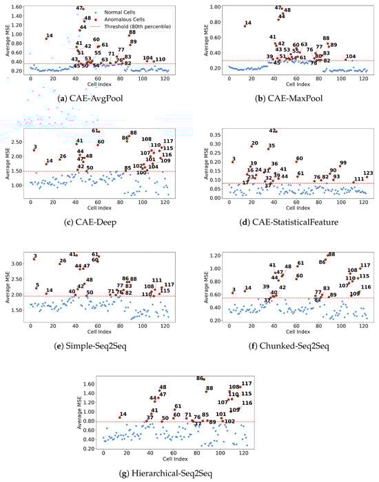
Figure 2.
Comparison of anomaly detection outcomes based on reconstruction errors from various autoencoder architectures. Each subplot corresponds to a different autoencoder method: (a) CAE-AvgPool, (b) CAE-MaxPool, (c) CAE-Deep, (d) CAE-StatisticalFeature, (e) Simple-Seq2Seq, (f) Chunked-Seq2Seq, and (g) Hierarchical-Seq2Seq. Blue points represent battery cells identified as normal, while red points indicate anomalous cells whose average mean squared error (MSE) exceeds the anomaly threshold, defined by the 80th percentile of reconstruction errors (shown as a red dashed line). Numbers next to red points specify the cell indices identified as anomalous. The figure illustrates distinct patterns in anomaly detection effectiveness across different autoencoder architectures, reflecting their varying strategies for dimensionality reduction and their capabilities in accurately reconstructing the battery cycle data.
For visual inspection, the data classified by the autoencoder as normal and anomalous are illustrated in Figure 3. In normal cell data (Figure 3a), the charge capacity (), discharge capacity (), and linearly interpolated discharge capacity () exhibit a gradual decline over successive cycles. Conversely, temperature-related features (T and linearly interpolated temperature, ) show an upward trend, aligning with typical degradation patterns observed in lithium-ion batteries under controlled cycling conditions [36]. These observations are consistent with established degradation mechanisms such as gradual capacity fade driven by incremental loss of lithium inventory and active material degradation [37]. In contrast, anomalous cell data (Figure 3b) exhibit irregular patterns across most features, except for the , which remains relatively stable. These irregularities may result from sensor malfunctions, manufacturing variability, or data acquisition errors. Notably, voltage (V) and current (I) profiles demonstrate abrupt fluctuations indicative of inconsistent charge-discharge dynamics that significantly deviate from typical lithium-ion cell operations. The abnormal temperature data (Figure 3c) specifically highlights deviations predominantly within temperature-related features, even though charge and discharge capacities remain within expected operational ranges. Such temperature anomalies could be attributed to environmental chamber temperature fluctuations previously identified in [24,34]. A particularly significant observation is the classification of the shortest end-of-life (EOL) cell (Figure 3d) as abnormal, despite initially following a capacity degradation trajectory resembling typical aging. This cell reached failure after just 148 cycles, considerably below the typical dataset range (150–2300 cycles). The autoencoder’s assignment of a high reconstruction error to this cell likely arises from its distinct degradation trajectory, which deviates from the typical patterns observed across the broader dataset. Overall, the presented results underscore the effectiveness of the autoencoder-based anomaly detection approach in differentiating between normal aging, irregular capacity fade, thermal anomalies, rapid EOL failures, and potential experimental irregularities.
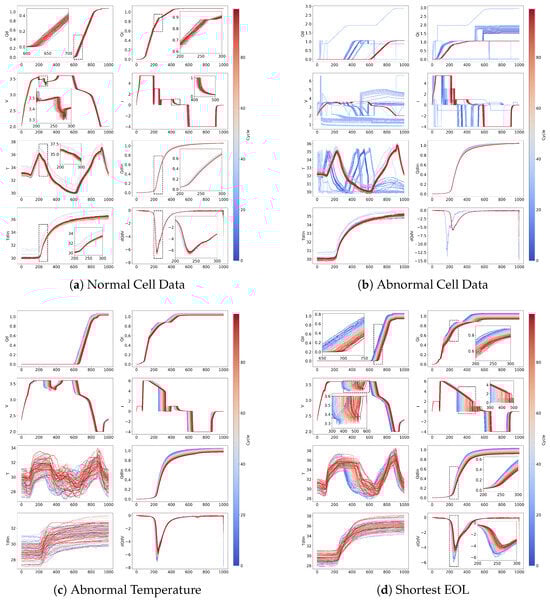
Figure 3.
Comparison of normal and abnormal battery cell data illustrating characteristic measurement patterns across cycles: (a) Normal cell data showing consistent, stable trends in charge capacity (QC), discharge capacity (QD), linearly interpolated discharge capacity (QDlin), voltage (V), current (I), temperature (T), and linearly interpolated temperature (Tdlin). (b) Abnormal cell data demonstrating irregularities, voltage spikes, and inconsistent patterns indicative of potential sensor or operational issues. (c) Abnormal temperature behavior specifically highlighting unusual temperature fluctuations that impact battery performance, consistent with previously reported anomalies [22,24]. (d) Battery cells with notably short end-of-life (EOL), exhibiting accelerated degradation or irregular trajectories compared to typical cells; these particular samples were typically excluded in previous studies [29,30]. In all subfigures, the color gradient (blue to red) corresponds to cycle indices, where blue represents earlier cycles and red indicates later cycles, clearly illustrating the evolution of battery measurements over time.
2.4. Preliminary Assessment of Dataset Quality and Feature Analysis
Random Forest (RF) models [38] were utilized to evaluate dataset effectiveness and to conduct feature importance analysis following the removal of anomalous cells from the dataset. The rationale for adopting RF models was twofold. First, RF models offer a computationally efficient approach to preliminarily assess the effectiveness of various anomaly detection methods applied to enhance dataset quality. Due to the significant computational requirements and prolonged training durations associated with DNNs, this preliminary assessment allows for the identification of the most promising anomaly detection methods. By quantifying the degree of improvement in dataset quality early in the analysis pipeline, researchers can make informed decisions to optimize computational resource allocation and streamline subsequent DNN training processes. Second, RF models inherently possess superior interpretability compared to DNNs. This interpretability is critical as it facilitates a comprehensive feature importance analysis, clarifying how specific features contribute to the predictive performance of the model. Consequently, RF-based feature importance analysis enhances the transparency of the modeling process and provides essential validation for the selected anomaly detection methods.
Table 3 summarizes the performance of RF models trained on datasets processed through various anomaly detection methods, evaluated using RMSE and MAPE metrics for both training and validation sets. For RUL prediction, the MAPE metric is particularly critical because RMSE values can be disproportionately influenced by cells with shorter EOL. In contrast, MAPE provides a relative measure of prediction accuracy that is less dependent on the variability in cell lifetimes, making it a more reliable and robust metric when evaluating predictive performance across datasets containing cells with diverse EOLs. RF models trained on standard datasets, comprising cycles 1–100 and cycles 21–120, yielded relatively lower errors on the training set but exhibited higher errors on the validation set. Observations indicating frequent anomalies within initial cycles informed the decision to exclude cycles 0–20. However, minimal performance improvement after this exclusion implies persistent data complexity and suggests caution regarding potential cycle-selection bias in future analyses. Datasets refined through autoencoder-based anomaly removal methods generally demonstrated improved predictive performance on the validation set, highlighting the effectiveness of these approaches. Among these methods, the CAE-StatisticalFeature approach yielded the lowest validation RMSE and a low validation MAPE. Similarly, the CAE-MaxPool method exhibited strong validation performance, validating its utility in enhancing dataset quality. Conversely, Seq2Seq approaches showed mixed results. Although the Simple-Seq2Seq method had relatively low training errors, validation errors remained relatively high. Chunked-Seq2Seq and Hierarchical-Seq2Seq methods produced higher validation errors, indicating challenges in effectively detecting anomalies within complex sequential data.
Table 3.
Performance comparison of Random Forest models trained on various datasets after anomaly removal.
Figure 4 presents a comparative analysis of feature importance derived from RF models across different datasets, utilizing SHapley Additive exPlanations (SHAP) and tree-based methodologies. All analyzed features originate from Lee et al. [34], with newly introduced features specifically highlighted in red to emphasize their novel contribution. Key features include internal resistance (IR), which indicates electrical resistance within the battery cell, as well as charge and discharge capacities (QC and QD), reflecting the battery’s capacity to store and deliver electrical charge, respectively. Temperature-related metrics such as average (), minimum (), and maximum () temperatures capture thermal behaviors throughout battery cycles. Additionally, incremental capacity features include average (), maximum (), and minimum () values. Current-related parameters, covering average and maximum values during both charge (, ) and discharge cycles (, ), further contribute insights into battery performance and stress conditions. Features newly introduced and emphasized by Lee et al. are distinctly highlighted in red within the figure. Figure 4a,b illustrate the feature importance scores for the dataset covering cycles 1–100. Both SHAP and tree-based analyses consistently identify newly introduced features from [34] (e.g., , and ) as highly significant predictors, validating their importance in battery degradation modeling. The alignment between SHAP and tree-based results strengthens the validity of the identified feature importance, as the convergence of two complementary methods reduces the likelihood of analytical bias. In Figure 4c,d, covering cycles 21–120, the same newly introduced features remain prominently influential, confirming their robustness across different cycle ranges. However, minor differences in feature rankings between methods and cycle ranges underline the sensitivity of these metrics to specific dataset configurations and reinforce the importance of employing multiple analytical methods. Figure 4e,f present feature importance scores after anomaly removal. Most significantly, the importance of the maximum temperature feature () substantially increases after filtering anomalies, suggesting that removing anomalous cells reveals the critical predictive role of temperature-related features.
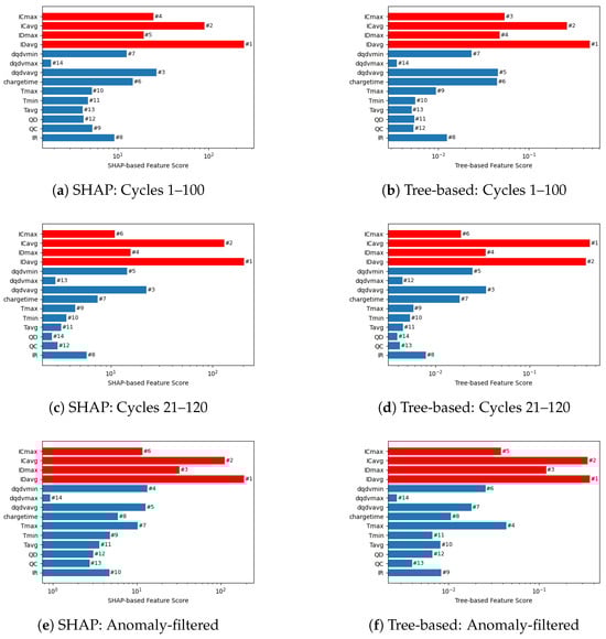
Figure 4.
Comparison of feature importance using SHAP and Tree-based methods across different cycle ranges and anomaly filtering conditions.
2.5. Deep Neural Network Training
The proposed model utilizes a ResNet-34-based architecture, adapted for one-dimensional convolutional processing. Residual connections inherent in ResNet architectures address the vanishing gradient problem, allowing the use of deeper neural networks that can extract complex, hierarchical temporal features. Each input sample is structured as a tensor of dimensions, where the first dimension (14) corresponds to distinct input features, and the second dimension represents a single channel suitable for 1D convolutional operations. The initial processing step involves a convolutional layer with 64 filters, a kernel size of 7, and a stride of 2, activated by the Rectified Linear Unit (ReLU). This convolutional operation is followed by a max-pooling layer with a pooling size of 3 and a stride of 2, reducing the temporal dimension while preserving critical feature representations. Subsequently, the network is organized into sequential stages comprising residual blocks designed for hierarchical temporal feature extraction. Stage 1 contains three residual blocks, each equipped with 64 filters. Stage 2 employs an initial convolutional layer with a stride of 2 to halve the temporal dimension, followed by three residual blocks comprising 128 filters each. Stage 3 further reduces the temporal dimension through an additional stride-2 convolutional layer, followed by seven residual blocks, each containing 256 filters, to capture higher-level temporal abstractions. Stage 4 comprises three residual blocks with 512 filters, providing deep-level feature extraction capabilities. Finally, a global average pooling layer aggregates temporal features, transforming them into a fixed-length vector that summarizes temporal information across all stages. A fully connected layer subsequently utilizes this aggregated vector to generate the final regression output. Overall, the described ResNet34-based model contains approximately 4.2 million trainable parameters Hyperparameter optimization of the ResNet architecture was performed using a systematic grid search approach. Prior research has extensively identified and evaluated the critical hyperparameters influencing model performance [34]. Building upon these established insights, the current study strategically narrowed its focus to optimize two pivotal hyperparameters: the implementation of batch normalization layers and the selection of optimal batch size.
Table 4 presents the comparative training and validation results of a ResNet model using data preprocessed by various autoencoder techniques. The baseline established by raw, unfiltered data exhibited high validation errors. The results indicate significant variability in ResNet performance depending on the preprocessing method employed. Among the convolutional autoencoder variations, CAE-Deep achieved better generalization than pooling-based CAE methods, as evidenced by lower validation errors. Conversely, pooling-based methods such as CAE-AvgPool and CAE-MaxPool yielded higher validation errors, suggesting limited effectiveness in capturing relevant features for this specific application. Notably, the Simple-Seq2Seq autoencoder consistently provided superior validation results, achieving the lowest validation without a k-fold split, thus indicating its potential as a robust preprocessing method. Interestingly, the analysis revealed increased validation errors across all methods when using the k-fold split, contrary to typical expectations that additional cross-validation splits enhance generalization. This finding underscores the necessity for careful selection and optimization of cross-validation parameters tailored to the specific dataset.
Table 4.
Training and validation performance of ResNet using data filtered by various autoencoders.
Table 5 presents a comparative analysis of performance metrics for various models. The baseline ResNet model, without any filtering, recorded comparatively higher errors, indicating limited predictive capability relative to the advanced architectures. The ResNet with Simple-Seq2Seq achieved the best performance, demonstrating the lowest error across all metrics. It is inherently challenging to explicitly attribute performance differences among autoencoder architectures due to the subtle and complex interactions among model design, hyperparameters, and data characteristics. However, given the sequential nature of battery degradation data, it is reasonable to infer that the Simple-Seq2Seq architecture’s explicit temporal modeling capability is crucial to its superior performance, as demonstrated consistently in our empirical evaluations. The ResNet with CAE-Deep and ResNet with CAE-StatisticalFeature models also showed notable performance improvements compared to basic ResNet models.
Table 5.
Performance metrics for different models.
Figure 5 provides an image visualization comparing cycle-by-cycle true and predicted remaining useful life (RUL) across multiple battery cells and cycles. This visualization is intended to provide an intuitive, qualitative overview of model accuracy differences between methods, complementing detailed numerical comparisons. Color intensity corresponds directly to RUL values: darker blue indicates lower RUL (approaching end-of-life), while lighter colors or red indicate higher RUL values (earlier in battery life). The subfigures contrast (a) the baseline ResNet model, which shows noticeable deviations and inconsistencies relative to the true RUL values, with (b) the ResNet integrated with Simple-Seq2Seq, clearly demonstrating improved accuracy and better alignment between predicted and true RUL values across battery cycles and cells.
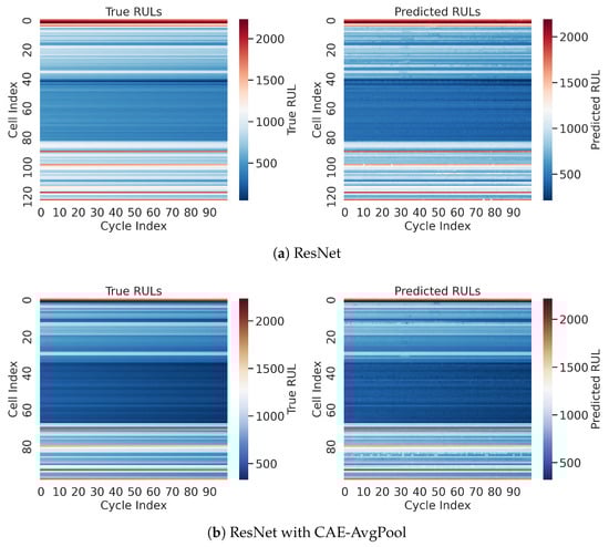
Figure 5.
Image visualization comparing cycle-by-cycle true and predicted RUL across battery cells and cycles for (a) ResNet and (b) ResNet with Simple-Seq2Seq.
Figure 6 provides a precise, quantitative evaluation of the models, presenting the distribution of cycle-by-cycle prediction errors between true and predicted RULs across individual cells for different model architectures. The ResNet with Simple-Seq2Seq architecture achieves the highest prediction accuracy and robustness, demonstrated by tighter error distributions and minimal maximum absolute errors within cycles across nearly all cells. Additionally, the ResNet with CAE-StatisticalFeature architecture shows strong stability, maintaining relatively small error distributions for most evaluated cells. Architectures such as ResNet with CAE-AvgPool, CAE-Deep, Chunked-Seq2Seq, and Hierarchical-Seq2Seq outperform the baseline ResNet, resulting in overall reduced prediction errors. However, these models occasionally produce noticeable outliers with higher maximum absolute errors for specific cells. These findings suggest that integrating a Simple-Seq2Seq architecture with ResNet significantly enhances predictive accuracy and reliability for RUL estimation.
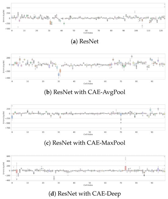
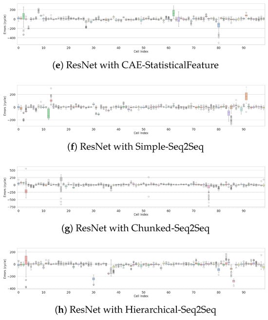
Figure 6.
Distribution of cycle-by-cycle prediction errors between true and predicted RUL across individual cells for various model architectures. The x-axis represents the cell index, and the y-axis shows prediction errors (in cycles) across all cycles for each cell.
3. Discussion
The proposed study significantly advances battery RUL prediction through a novel integration of anomaly detection techniques using diverse autoencoder architectures combined with a ResNet-based deep neural network model. This research highlights substantial progress in predictive reliability for EV and ESS applications by achieving state-of-the-art accuracy in cycle-by-cycle battery RUL prediction.
The ResNet model, integrated with the Simple-Seq2Seq autoencoder, was identified as the most accurate and stable model, providing lower prediction errors across multiple metrics and minimal maximum absolute errors. This stability is particularly crucial for safety-critical applications, such as EVs, where the consistent and reliable prediction of battery health impacts operational safety, prevents unexpected failures, and ensures overall system reliability. CAE-AvgPool and CAE-MaxPool exhibited comparatively limited effectiveness, likely due to the potential loss of critical transient information during the pooling process. Conversely, the CAE-StatisticalFeature architecture was robust in filtering anomalies, underlining its potential for computational efficiency and reliable anomaly detection.
The systematic anomaly filtering approach, integrated through autoencoders, reduced potential biases associated with sample selection. This finding represents an indirect yet practical validation of autoencoder applications for real-world anomaly detection, as evidenced by the clear performance improvement when comparing the baseline ResNet performance to that of anomaly-filtered models. The chosen anomaly detection threshold—set at the 80th percentile of reconstruction errors—was intentionally selected to transparently demonstrate the beneficial effect of autoencoder-based filtering rather than to establish optimal anomaly detection performance metrics. Future research could benefit from integrating advanced anomaly detection strategies, such as hybrid models, probabilistic frameworks, and dynamic thresholding approaches [11], to further enhance accuracy.
Despite achieving significant advancements, the persistent gap between training and validation errors indicates the need for more comprehensive datasets. Increasing validation errors with higher k-fold splits further support the necessity for expanded datasets to enhance model generalizability and accuracy. Future studies should therefore continue to explore advanced anomaly detection methodologies, assess their applicability across varied operational conditions and battery chemistries, and leverage larger datasets to ensure improved robustness and enhanced real-world predictive performance.
4. Conclusions
This study proposes a deep learning framework that combines autoencoder-based anomaly detection with a ResNet-based neural network for accurate and reliable cycle-by-cycle RUL prediction of lithium-ion batteries. By integrating anomaly detection into the preprocessing pipeline, the framework effectively addresses the challenges of anomalous battery data, resulting in significantly enhanced prediction stability and accuracy. Among the tested architectures, the Simple-Seq2Seq autoencoder proved most effective, yielding the lowest prediction errors and demonstrating superior generalization performance.
A key strength of the methodology lies in its systematic approach to identifying and filtering anomalous data, which improves dataset quality and model robustness. The experimental results confirm the effectiveness of the proposed framework, achieving an MAPE of 2.85% and an RMSE of 40.87 cycles, outperforming prior single-cycle RUL prediction studies. The results highlight the importance of comprehensive preprocessing and anomaly management in enhancing predictive reliability in real-world applications.
While this study focuses on convolutional and sequence-based autoencoder architectures, other promising variants, such as variational and adversarial autoencoders, were not explored due to the significant time and computational resources required for their training and optimization. Future work will aim to extend the framework by incorporating these advanced architectures, along with adaptive thresholding techniques and hybrid anomaly detection strategies.
Author Contributions
Conceptualization, J.L. (Junghwan Lee); methodology, J.L. (Junghwan Lee); software, J.L. (Junghwan Lee), B.L. and D.K.; validation, J.L. (Junghwan Lee), L.W. and J.L. (Jiaxin Liu); formal analysis, J.L. (Junghwan Lee); investigation, J.L. (Junghwan Lee) and H.J.; resources, D.K. and B.L.; data curation, J.L. (Junghwan Lee), D.K. and B.L.; writing—original draft preparation, J.L. (Junghwan Lee); writing—review and editing, J.L. (Junghwan Lee), L.W. and J.L. (Jong Lim); visualization, J.L. (Junghwan Lee) and J.L. (Jiaxin Liu); supervision, J.L. (Junghwan Lee); project administration, J.L. (Junghwan Lee); funding acquisition, H.J. All authors have read and agreed to the published version of the manuscript.
Funding
This work was part of the BatterMachine research and development project funded by the Korea Technology & Information Promotion Agency for SMEs of South Korea (Grant No. 00442413).
Data Availability Statement
Codes are available on GitHub: https://github.com/BatterMachineCo/dnn_autoencoders.git GitHub Repository, accessed on 27 July 2025.
Conflicts of Interest
Authors Junghwan Lee, Hoseok Jung, Bukyu Lim, Dael Kim and Jong Lim were employed by the company Research and Development Department, Batter Machine Co., Ltd. Authors Junghwan Lee and Jiaxin Liu were employed by the company Livision AI Technology Co., Ltd. The remaining author declares that the research was conducted in the absence of any commercial or financial relationships that could be construed as a potential conflict of interest.
Appendix A
The autoencoder architectures evaluated in this study utilize two distinct types of input data:
- Time-Series Input (used by CAE-AvgPool, CAE-MaxPool, CAE-Deep, Simple-Seq2Seq, Chunked-Seq2Seq, Hierarchical-Seq2Seq): Each input sample has dimensions of (None, 1000, 8), representing battery cycle measurements over 1000 time-steps, with the following eight sequential features per step:
- Voltage
- Current
- Temperature
- Integrated charge capacity (QC)
- Integrated discharge capacity (QD)
- Linearly interpolated discharge capacity (QDlin)
- Linearly interpolated temperature (Tdlin)
- Internal resistance (IR)
- Statistical Feature Input (CAE-StatisticalFeature only): This input consists of a single timestep per cycle with 14 summary statistics derived from each battery cycle, matching the features utilized in the ResNet model for RUL prediction:
- Average voltage
- Maximum voltage
- Minimum voltage
- Average temperature
- Maximum temperature
- Minimum temperature
- Integrated charge capacity (QC)
- Integrated discharge capacity (QD)
- Linearly interpolated discharge capacity (QDlin)
- Linearly interpolated temperature (Tdlin)
- Internal resistance (IR)
- Average incremental capacity (dQ/dV)
- Maximum incremental capacity (dQ/dV)
- Minimum incremental capacity (dQ/dV)
Table A1.
The architecture consists of convolutional layers with progressively increasing filters, batch normalization for stable training, average pooling layers for dimensionality reduction, and upsampling layers for reconstruction.
Table A1.
The architecture consists of convolutional layers with progressively increasing filters, batch normalization for stable training, average pooling layers for dimensionality reduction, and upsampling layers for reconstruction.
| Layer (Type) | Output Shape | Number of Parameters |
|---|---|---|
| InputLayer | (None, 1000, 8) | 0 |
| Conv1D | (None, 1000, 32) | 800 |
| BatchNormalization | (None, 1000, 32) | 128 |
| AveragePooling1D | (None, 500, 32) | 0 |
| Conv1D | (None, 500, 64) | 6208 |
| BatchNormalization | (None, 500, 64) | 256 |
| AveragePooling1D | (None, 250, 64) | 0 |
| Conv1D | (None, 250, 128) | 24,704 |
| BatchNormalization | (None, 250, 128) | 512 |
| AveragePooling1D | (None, 125, 128) | 0 |
| UpSampling1D | (None, 250, 128) | 0 |
| Conv1D | (None, 250, 64) | 24,640 |
| BatchNormalization | (None, 250, 64) | 256 |
| UpSampling1D | (None, 500, 64) | 0 |
| Conv1D | (None, 500, 32) | 6176 |
| BatchNormalization | (None, 500, 32) | 128 |
| UpSampling1D | (None, 1000, 32) | 0 |
| Conv1D | (None, 1000, 8) | 776 |
| BatchNormalization | (None, 1000, 8) | 32 |
Table A2.
The model architecture utilizes convolutional layers, batch normalization, max pooling for dimensionality reduction, and upsampling for reconstructing the input dimensions.
Table A2.
The model architecture utilizes convolutional layers, batch normalization, max pooling for dimensionality reduction, and upsampling for reconstructing the input dimensions.
| Layer (Type) | Output Shape | Number of Parameters |
|---|---|---|
| InputLayer | (None, 1000, 8) | 0 |
| Conv1D | (None, 1000, 8) | 648 |
| BatchNormalization | (None, 1000, 8) | 32 |
| MaxPooling1D | (None, 100, 8) | 0 |
| Conv1D | (None, 100, 8) | 648 |
| BatchNormalization | (None, 100, 8) | 32 |
| MaxPooling1D | (None, 10, 8) | 0 |
| Conv1D | (None, 10, 8) | 648 |
| BatchNormalization | (None, 10, 8) | 32 |
| MaxPooling1D | (None, 1, 8) | 0 |
| UpSampling1D | (None, 10, 8) | 0 |
| Conv1D | (None, 10, 8) | 648 |
| BatchNormalization | (None, 10, 8) | 32 |
| UpSampling1D | (None, 100, 8) | 0 |
| Conv1D | (None, 100, 8) | 648 |
| BatchNormalization | (None, 100, 8) | 32 |
| UpSampling1D | (None, 1000, 8) | 0 |
| Conv1D | (None, 1000, 8) | 648 |
| BatchNormalization | (None, 1000, 8) | 32 |
Table A3.
This deep convolutional autoencoder architecture employs multiple convolutional layers with increasing filters to capture hierarchical feature representations, followed by average pooling layers for dimensionality reduction, and corresponding upsampling and convolutional layers for accurate reconstruction.
| Layer (Type) | Output Shape | Number of Parameters |
|---|---|---|
| InputLayer | (None, 1000, 8) | 0 |
| Conv1D | (None, 1000, 128) | 10,368 |
| BatchNormalization | (None, 1000, 128) | 512 |
| AveragePooling1D | (None, 100, 128) | 0 |
| Conv1D | (None, 100, 64) | 81,984 |
| BatchNormalization | (None, 100, 64) | 256 |
| AveragePooling1D | (None, 10, 64) | 0 |
| Conv1D | (None, 10, 32) | 20,512 |
| BatchNormalization | (None, 10, 32) | 128 |
| AveragePooling1D | (None, 1, 32) | 0 |
| Conv1D | (None, 1, 16) | 528 |
| UpSampling1D | (None, 10, 16) | 0 |
| Conv1D | (None, 10, 32) | 5152 |
| BatchNormalization | (None, 10, 32) | 128 |
| UpSampling1D | (None, 100, 32) | 0 |
| Conv1D | (None, 100, 64) | 20,544 |
| BatchNormalization | (None, 100, 64) | 256 |
| UpSampling1D | (None, 1000, 64) | 0 |
| Conv1D | (None, 1000, 128) | 82,048 |
| BatchNormalization | (None, 1000, 128) | 512 |
| Conv1D | (None, 1000, 8) | 1032 |
Table A4.
This architecture employs LSTM layers to capture sequential dependencies, compressing and subsequently reconstructing the input sequences.
Table A4.
This architecture employs LSTM layers to capture sequential dependencies, compressing and subsequently reconstructing the input sequences.
| Layer (Type) | Output Shape | Number of Parameters |
|---|---|---|
| InputLayer | (None, 1000, 8) | 0 |
| LSTM (Encoder) | (None, 8) | 544 |
| RepeatVector | (None, 1000, 8) | 0 |
| LSTM (Decoder) | (None, 1000, 8) | 544 |
Table A5.
The architecture splits input sequences into chunks for localized sequential modeling, utilizing TimeDistributed LSTM layers to process each chunk individually and reconstruct the original data shape.
Table A5.
The architecture splits input sequences into chunks for localized sequential modeling, utilizing TimeDistributed LSTM layers to process each chunk individually and reconstruct the original data shape.
| Layer (Type) | Output Shape | Number of Parameters |
|---|---|---|
| InputLayer | (None, 1000, 8) | 0 |
| Reshape | (None, 10, 100, 8) | 0 |
| TimeDistributed (LSTM Encoder) | (None, 10, 8) | 544 |
| TimeDistributed (RepeatVector) | (None, 10, 100, 8) | 0 |
| Reshape | (None, 10, 100, 8) | 0 |
| TimeDistributed (LSTM Decoder) | (None, 10, 100, 8) | 544 |
| Reshape | (None, 1000, 8) | 0 |
Table A6.
This hierarchical sequence-to-sequence model captures both local and global temporal dependencies by processing segmented data chunks through TimeDistributed and LSTM layers, enabling detailed reconstruction of the input sequence.
Table A6.
This hierarchical sequence-to-sequence model captures both local and global temporal dependencies by processing segmented data chunks through TimeDistributed and LSTM layers, enabling detailed reconstruction of the input sequence.
| Layer (Type) | Output Shape | Number of Parameters |
|---|---|---|
| InputLayer | (None, 1000, 8) | 0 |
| Reshape | (None, 10, 100, 8) | 0 |
| TimeDistributed (LSTM Encoder) | (None, 10, 8) | 544 |
| LSTM (Global Encoder) | (None, 8) | 544 |
| RepeatVector | (None, 10, 8) | 0 |
| LSTM (Global Decoder) | (None, 10, 8) | 544 |
| TimeDistributed (RepeatVector) | (None, 10, 100, 8) | 0 |
| Reshape | (None, 10, 100, 8) | 0 |
| TimeDistributed (LSTM Decoder) | (None, 10, 100, 8) | 544 |
| Reshape | (None, 1000, 8) | 0 |
Table A7.
The architecture utilizes convolutional layers with batch normalization for feature extraction, pooling layers for dimensionality reduction, and upsampling layers with convolutional operations followed by a dense layer for reconstruction of statistical input features.
Table A7.
The architecture utilizes convolutional layers with batch normalization for feature extraction, pooling layers for dimensionality reduction, and upsampling layers with convolutional operations followed by a dense layer for reconstruction of statistical input features.
| Layer (Type) | Output Shape | Number of Parameters |
|---|---|---|
| InputLayer | (None, 14, 1) | 0 |
| Conv1D | (None, 7, 128) | 512 |
| BatchNormalization | (None, 7, 128) | 512 |
| Conv1D | (None, 4, 64) | 24,640 |
| BatchNormalization | (None, 4, 64) | 256 |
| Conv1D | (None, 2, 32) | 6176 |
| BatchNormalization | (None, 2, 32) | 128 |
| Conv1D | (None, 2, 16) | 1552 |
| BatchNormalization | (None, 2, 16) | 64 |
| Conv1D | (None, 2, 1) | 17 |
| UpSampling1D | (None, 4, 1) | 0 |
| Conv1D | (None, 4, 16) | 64 |
| BatchNormalization | (None, 4, 16) | 64 |
| UpSampling1D | (None, 8, 16) | 0 |
| Conv1D | (None, 8, 32) | 1568 |
| BatchNormalization | (None, 8, 32) | 128 |
| UpSampling1D | (None, 16, 32) | 0 |
| Conv1D | (None, 16, 64) | 6208 |
| BatchNormalization | (None, 16, 64) | 256 |
| Conv1D | (None, 16, 128) | 24,704 |
| Flatten | (None, 2048) | 0 |
| Dense | (None, 14) | 28,686 |
| Reshape | (None, 14, 1) | 0 |
References
- Bose, B.; Shaosen, S.; Li, W.; Gao, L.; Wei, K.; Garg, A. Cloud-Battery management system based health-aware battery fast charging architecture using error-correction strategy for electric vehicles. Sustain. Energy Grids Netw. 2023, 36, 101197. [Google Scholar] [CrossRef]
- Lee, J.; Sun, H.; Liu, Y.; Li, X.; Liu, Y.; Kim, M. State-of-Health Estimation and Anomaly Detection in Li-Ion Batteries Based on a Novel Architecture with Machine Learning. Batteries 2023, 9, 264. [Google Scholar] [CrossRef]
- Sulzer, V.; Mohtat, P.; Aitio, A.; Lee, S.; Yeh, Y.T.; Steinbacher, F.; Khan, M.U.; Lee, J.W.; Siegel, J.B.; Stefanopoulou, A.G.; et al. The challenge and opportunity of battery lifetime prediction from field data. Joule 2021, 5, 1934–1955. [Google Scholar] [CrossRef]
- Chen, K.; Zhu, J.; Zhou, S.; Liu, K.; Gao, B.; Gao, G.; Wu, G. Impedance estimation for lithium-ion battery using support vector regression and cuckoo search algorithm. CSEE J. Power Energy Syst. 2023. [Google Scholar] [CrossRef]
- Li, Y.; Gao, G.; Chen, K.; He, S.; Liu, K.; Xin, D.; Luo, Y.; Long, Z.; Wu, G. State-of-health prediction of lithium-ion batteries using feature fusion and a hybrid neural network model. Energy 2025, 319, 135163. [Google Scholar] [CrossRef]
- Ren, L.; Dong, J.; Wang, X.; Meng, Z.; Zhao, L.; Deen, M.J. A Data-Driven Auto-CNN-LSTM Prediction Model for Lithium-Ion Battery Remaining Useful Life. IEEE Trans. Ind. Inform. 2021, 17, 3478–3487. [Google Scholar] [CrossRef]
- Zhang, J.; Wang, Y.; Jiang, B.; He, H.; Huang, S.; Wang, C.; Zhang, Y.; Han, X.; Guo, D.; He, G.; et al. Realistic Fault Detection of Li-Ion Battery via Dynamical Deep Learning. Nat. Commun. 2023, 14, 5940. [Google Scholar] [CrossRef]
- Xia, W.; Xu, J.; Liu, B.; Duan, H. A Novel Denoising Autoencoder Hybrid Network for Remaining Useful Life Estimation of Lithium-Ion Batteries. Energy Sci. Eng. 2024, 12, 3390–3400. [Google Scholar] [CrossRef]
- Hong, S.; Kang, M.; Kim, J.; Baek, J. Sequential Application of Denoising Autoencoder and Long-Short Recurrent Convolutional Network for Noise-Robust Remaining-Useful-Life Prediction Framework of Lithium-Ion Batteries. Comput. Ind. Eng. 2023, 179, 109231. [Google Scholar] [CrossRef]
- Jeon, J.; Cheon, H.; Jung, B.; Kim, H. ProADD: Proactive Battery Anomaly Dual Detection Leveraging Denoising Convolutional Autoencoder and Incremental Voltage Analysis. Appl. Energy 2024, 373, 123757. [Google Scholar] [CrossRef]
- Sun, C.; He, Z.; Lin, H.; Cai, L.; Cai, H.; Gao, M. Anomaly Detection of Power Battery Pack Using Gated Recurrent Units Based Variational Autoencoder. Appl. Soft Comput. 2023, 132, 109903. [Google Scholar] [CrossRef]
- He, X.; Sun, B.; Zhang, W.; Su, X.; Ma, S.; Li, H.; Ruan, H. Inconsistency Modeling of Lithium-Ion Battery Pack Based on Variational Auto-Encoder Considering Multi-Parameter Correlation. Energy 2023, 277, 127409. [Google Scholar] [CrossRef]
- Tao, S.; Ma, R.; Zhao, Z.; Ma, G.; Su, L.; Chang, H.; Chen, Y.; Liu, H.; Liang, Z.; Cao, T.; et al. Generative Learning Assisted State-of-Health Estimation for Sustainable Battery Recycling with Random Retirement Conditions. Nat. Commun. 2024, 15, 10154. [Google Scholar] [CrossRef] [PubMed]
- Chan, J.; Han, T.; Pan, E. Variational Autoencoder-Driven Adversarial SVDD for Power Battery Anomaly Detection on Real Industrial Data. J. Energy Storage 2024, 103, 114267. [Google Scholar] [CrossRef]
- Jiao, R.; Peng, K.; Dong, J. Remaining Useful Life Prediction of Lithium-Ion Batteries Based on Conditional Variational Autoencoders-Particle Filter. IEEE Trans. Instrum. Meas. 2020, 69, 8831–8843. [Google Scholar] [CrossRef]
- Zhang, H.; Guo, K.; Chen, Y.; Sun, J. Remaining Useful-Life Prediction of Lithium Battery Based on Neural-Network Ensemble via Conditional Variational Autoencoder. Appl. Intell. 2025, 55, 34. [Google Scholar] [CrossRef]
- Cai, L.; Li, J.; Xu, X.; Jin, H.; Meng, J.; Wang, B.; Wu, C.; Yang, S. Automatically Constructing a Health Indicator for Lithium-Ion Battery State-of-Health Estimation via Adversarial and Compound Stacked Autoencoder. J. Energy Storage 2024, 84, 110711. [Google Scholar] [CrossRef]
- Cai, L.; Yan, J.; Jin, H.; Meng, J.; Peng, J.; Wang, B.; Liang, W.; Teodorescu, R. A Two-Stage Method with Twin Autoencoders for the Degradation Trajectories Prediction of Lithium-Ion Batteries. J. Energy Chem. 2025, 103, 759–772. [Google Scholar] [CrossRef]
- Guille-Escuret, C.; Rodriguez, P.; Vazquez, D.; Mitliagkas, I.; Monteiro, J. CADet: Fully Self-Supervised Anomaly Detection with Contrastive Learning. In Proceedings of the Advances in Neural Information Processing Systems 36 (NeurIPS 2023), New Orleans, LA, USA, 10–16 December 2023; Curran Associates Inc.: Red Hook, NY, USA, 2023. [Google Scholar]
- Raghuram, J.; Chandrasekaran, V.; Jha, S.; Banerjee, S. A General Framework For Detecting Anomalous Inputs to DNN Classifiers. In Proceedings of the 38th International Conference on Machine Learning (ICML 2021), Virtual, 18–24 July 2021; Volume 139, pp. 8764–8775. [Google Scholar]
- de la Iglesia, D.H.; Corbacho, C.C.; Dib, J.Z.; Alonso-Secades, V.; López Rivero, A.J. Advanced Machine Learning and Deep Learning Approaches for Estimating the Remaining Life of EV Batteries—A Review. Batteries 2025, 11, 17. [Google Scholar] [CrossRef]
- Severson, K.A.; Attia, P.M.; Jin, N.; Perkins, N.; Jiang, B.; Yang, Z.; Chen, M.H.; Aykol, M.; Herring, P.K.; Fraggedakis, D.; et al. Data-driven prediction of battery cycle life before capacity degradation. Nat. Energy 2019, 4, 383–391. [Google Scholar] [CrossRef]
- Lu, J.; Xiong, R.; Tian, J.; Wang, C.; Hsu, C.W.; Tsou, N.T.; Sun, F.; Li, J. Battery degradation prediction against uncertain future conditions with recurrent neural network enabled deep learning. Energy Storage Mater. 2022, 50, 139–151. [Google Scholar] [CrossRef]
- Hsu, C.W.; Xiong, R.; Chen, N.Y.; Li, J.; Tsou, N.T. Deep neural network battery life and voltage prediction by using data of one cycle only. Appl. Energy 2022, 306, 118134. [Google Scholar] [CrossRef]
- Segler, M.H.S.; Preuss, M.; Waller, M.P. Planning chemical syntheses with deep neural networks and symbolic AI. Nature 2018, 555, 604–610. [Google Scholar] [CrossRef]
- Tang, Y.; Yang, K.; Zheng, H.; Zhang, S.; Zhang, Z. Early prediction of lithium-ion battery lifetime via a hybrid deep learning model. Measurement 2022, 199, 111530. [Google Scholar] [CrossRef]
- Couture, J.; Lin, X. Image- and health indicator-based transfer learning hybridization for battery RUL prediction. Eng. Appl. Artif. Intell. 2022, 114, 105120. [Google Scholar] [CrossRef]
- Safavi, V.; Mohammadi Vaniar, A.; Bazmohammadi, N.; Vasquez, J.C.; Keysan, O.; Guerrero, J.M. Early prediction of battery remaining useful life using CNN-XGBoost model and Coati optimization algorithm. J. Energy Storage 2024, 98, 113176. [Google Scholar] [CrossRef]
- Gong, D.; Gao, Y.; Kou, Y.; Wang, Y. Early prediction of cycle life for lithium-ion batteries based on evolutionary computation and machine learning. J. Energy Storage 2022, 51, 104376. [Google Scholar] [CrossRef]
- Fei, Z.; Zhang, Z.; Yang, F.; Tsui, K.L.; Li, L. Early-stage lifetime prediction for lithium-ion batteries: A deep learning framework jointly considering machine-learned and handcrafted data features. J. Energy Storage 2022, 52, 104936. [Google Scholar] [CrossRef]
- Sanz-Gorrachategui, I.; Wang, Y.; Guillén-Asensio, A.; Bono-Nuez, A.; Martín-del Brío, B.; Orlik, P.V.; Pastor-Flores, P. Remaining Useful Life Estimation of Used Li-Ion Cells With Deep Learning Algorithms Without First Life Information. IEEE Access 2024, 12, 147798–147808. [Google Scholar] [CrossRef]
- Yang, X.; Xie, H.; Zhang, L.; Yang, K.; Liu, Y.; Chen, G.; Ma, B.; Liu, X.; Chen, S. Early-stage degradation trajectory prediction for lithium-ion batteries: A generalized method across diverse operational conditions. J. Power Sources 2024, 612, 234808. [Google Scholar] [CrossRef]
- Zhang, Q.; Yang, L.; Guo, W.; Qiang, J.; Peng, C.; Li, Q.; Deng, Z. A deep learning method for lithium-ion battery remaining useful life prediction based on sparse segment data via cloud computing system. Energy 2022, 241, 122716. [Google Scholar] [CrossRef]
- Lee, J.; Sun, H.; Liu, Y.; Li, X. A machine learning framework for remaining useful lifetime prediction of li-ion batteries using diverse neural networks. Energy AI 2024, 15, 100319. [Google Scholar] [CrossRef]
- Cao, R.; Zhang, Z.; Shi, R.; Lu, J.; Zheng, Y.; Sun, Y.; Liu, X.; Yang, S. Model-Constrained Deep Learning for Online Fault Diagnosis in Li-Ion Batteries Over Stochastic Conditions. Nat. Commun. 2025, 16, 1651. [Google Scholar] [CrossRef] [PubMed]
- Attia, P.M.; Grover, A.; Jin, N.; Severson, K.A.; Markov, T.M.; Liao, Y.H.; Chen, M.H.; Cheong, B.; Perkins, N.; Yang, Z.; et al. Closed-loop optimization of fast-charging protocols for batteries with machine learning. Nature 2020, 578, 397–402. [Google Scholar] [CrossRef] [PubMed]
- Tebbe, J.; Hartwig, A.; Jamali, A.; Senobar, H.; Wahab, A.; Kabak, M.; Kemper, H.; Khayyam, H. Innovations and prognostics in battery degradation and longevity for energy storage systems. J. Energy Storage 2025, 114, 115724. [Google Scholar] [CrossRef]
- Pedregosa, F.; Varoquaux, G.; Gramfort, A.; Michel, V.; Thirion, B.; Grisel, O.; Blondel, M.; Prettenhofer, P.; Weiss, R.; Dubourg, V.; et al. Scikit-learn: Machine Learning in Python. J. Mach. Learn. Res. 2011, 12, 2825–2830. [Google Scholar]
Disclaimer/Publisher’s Note: The statements, opinions and data contained in all publications are solely those of the individual author(s) and contributor(s) and not of MDPI and/or the editor(s). MDPI and/or the editor(s) disclaim responsibility for any injury to people or property resulting from any ideas, methods, instructions or products referred to in the content. |
© 2025 by the authors. Licensee MDPI, Basel, Switzerland. This article is an open access article distributed under the terms and conditions of the Creative Commons Attribution (CC BY) license (https://creativecommons.org/licenses/by/4.0/).