State-of-Health Estimation for Lithium-Ion Batteries via Incremental Energy Analysis and Hybrid Deep Learning Model

Abstract

Accurate State-of-Health (SOH) estimation is a key technology for ensuring battery safety, optimizing energy management, and enhancing lifecycle value. This paper proposes a novel SOH estimation method for lithium-ion batteries, utilizing incremental energy features and a hybrid deep learning model that combines Convolutional Neural Network (CNN), Kolmogorov–Arnold Network (KAN), and Bidirectional Long Short-Term Memory (BiLSTM) (CNN-KAN-BiLSTM). First, the battery’s voltage, current, temperature, and other data during the charging stage were measured and recorded through experiments. Incremental Energy Analysis (IEA) was conducted on the charging data to extract various incremental energy characteristics. The Pearson correlation method was used to verify the strong correlation between the proposed characteristics and the battery SOH. This paper includes experimental verification of the method for both battery cells and battery pack. For the battery cell, a complete multi-feature sequence was formed based on the incremental energy curve characteristics combined with temperature characteristics. For the battery pack, the characteristics of the incremental energy curve were supplemented with Variance of Voltage Means (VVM) as an inconsistent feature, combined with Standard Deviation of Temperature Means (SDTM), to create a complete multi-feature sequence. The features were then input into the CNN-KAN-BiLSTM deep learning model developed in this study for training, successfully estimating the SOH of lithium batteries. The results demonstrate that the proposed method can accurately estimate the SOH of lithium batteries, even though the SOH degradation of lithium batteries has significant nonlinear characteristics. The Mean Absolute Error (MAE) and Root Mean Square Error (RMSE) for the lithium battery pack were 0.3910 and 0.4797, respectively, with an average coefficient of determination (R²) exceeding 99%. The final SOH estimation MAE values for battery cells at different charging rates of 0.1 C (250 mA), 0.2 C (500 mA), and 0.5 C (1250 mA) were 0.2728, 0.3301, and 0.2094. The RMSE were 0.3792, 0.4494, and 0.2699, respectively. The corresponding R² values were 98.76%, 97.07%, and 99.37%, respectively. Finally, the effectiveness and universality of the method proposed in this paper were verified using the NASA battery dataset and the CALCE battery dataset.

1. Introduction

Accurate, efficient, and reliable estimation of the State-of-Health (SOH) of lithium-ion batteries is critical for enhancing the range and service life of electric vehicles. Economically, SOH estimation extends battery life, reduces maintenance costs, and facilitates cascade utilization. With the rapid development of new energy vehicles, SOH estimation has emerged as a key supporting technology that promotes the sustainable advancement of the industry and contributes to the goal of carbon neutrality, offering both commercial value and social benefits [1,2,3,4,5,6]. There are various definitions for the SOH of batteries. This paper uses the capacity ratio to define the SOH of lithium-ion batteries. This definition is both intuitive and reliable, as shown in Equation (1):

$$SOH={\displaystyle \frac{Q_{\max \mathrm{capacity}}}{Q_{\mathrm{rated}\mathrm{capacity}}}}\times 100\%$$

(1)

where $Q_{\max \mathrm{capacity}}$ indicates the current maximum discharge capacity of a lithium battery, and $Q_{\mathrm{rated}\mathrm{capacity}}$ indicates the rated capacity of the lithium battery.

In recent years, numerous domestic and foreign scholars have proposed various estimation methods for assessing the health status of lithium batteries [7,8]. These methods can be categorized into three main types: direct measurement, model-based, and data-driven approaches. The primary direct measurement techniques include Coulomb counting [8], open-circuit voltage (OCV) [9], and electrochemical impedance spectroscopy [10,11,12]. Among these, the Coulomb counting method estimates the capacity decay rate by integrating the current. While this method is straightforward, it is susceptible to inaccuracies due to sensor precision, integral error, and self-discharge effects, and thus, its long-term accuracy is limited. The open-circuit voltage method evaluates the SOH based on the OCV-SOC [13] curve deviation after the battery has rested. However, this method requires a long static equilibrium time and is susceptible to temperature variations, SOC errors, and polarization interference, resulting in low dynamic applicability. Electrochemical impedance spectroscopy (EIS) analyzes the aging mechanism by extracting impedance parameters, such as ohmic and charge-transfer impedance, through AC excitation. This method is highly dependent on equipment accuracy, and the algorithm is complex, posing significant challenges due to high cost and high-frequency noise interference, making its real-time application difficult.

Model-based methods [14,15] can be roughly categorized into three types: empirical models [14], equivalent circuit models [16,17], and electrochemical models [18]. The empirical model relies on experimental data to fit the aging law, such as capacity decay and internal resistance growth, and establishes a statistical relationship between SOH, cycle times, temperature, and other parameters. While this model is computationally efficient and easy to deploy, it is limited by the data range, cannot analyze the aging mechanism, and exhibits significant errors when the data boundary is exceeded. The equivalent circuit model uses a resistance–capacitance network (such as the Rint model) to mathematically characterize the dynamic characteristics of the battery. It enables the quantitative estimation of the battery’s SOH through real-time online identification of characteristic parameters, such as ohmic internal resistance. This approach is both real-time and physically explanatory; however, identifying parameters in higher-order models can be challenging, and the simulation accuracy for high-frequency responses is often limited. The electrochemical model is based on the porous electrode theory, quantifying microscopic processes such as lithium-ion diffusion and aging mechanisms (such as lithium deposition), and constructing partial differential equations (such as the P2D model). The mechanism is clear, but the calculation is complex. It is only applicable to laboratory research and difficult to apply in real-time vehicles.

The data-driven method [19,20,21,22,23,24,25] relies on historical operational data from the battery to extract the corresponding features and directly builds an SOH estimation model based on machine learning algorithms, thereby avoiding the complexities of the physical modeling [26] process. Traditionally, extracted features include current, voltage, and temperature; however, these metrics lack mechanistic characteristics. The common incremental capacity analysis (ICA) method is based on the voltage–capacity relationship. By plotting the incremental capacity (IC) curve, key change points in the SOH degradation process can be identified. This method indirectly characterizes the equilibrium of internal chemical reactions and offers good physical interpretability. However, ICA only analyzes the relationship between capacity and voltage, ignoring changes in battery energy, which is a more comprehensive indicator of battery performance. Data-driven methods mainly include Support Vector Machine (SVM) [27], Random Forest (RF) [28,29], etc. Although SVM shows good classification and regression performance on medium and small-scale datasets, due to its high dependence on input features and kernel function selection, it is difficult to accurately depict the timing law of battery SOH changes using the number of cycles. At the same time, the computational cost is relatively high when dealing with high-dimensional and diverse battery data, which restricts the wide application of this method in engineering practice. Although RF has strong nonlinear modeling ability and the advantage of resisting overfitting, its nature as a static integrated model makes it difficult to effectively learn the temporal correlation characteristics in the degradation process of battery SOH. Furthermore, when dealing with data from different battery models or working conditions, this model has insufficient generalization performance, and the prediction results are prone to discontinuous fluctuations, thereby reducing the stability of state estimation. These traditional machine learning methods often show obvious limitations in dealing with complex nonlinear and time-varying characteristics. In recent years, deep learning techniques [26,30,31,32,33], such as Long Short-Term Memory (LSTM) [34,35], Gated Recurrent Unit (GRU) [36,37], and Transformer [38,39], have emerged. Although LSTM can effectively model the dependencies of a long-term series, when dealing with data such as battery SOH, that degrade slowly and evolve over a long period of time, it still faces the problem of memory capacity attenuation caused by vanishing gradients. Meanwhile, this model is highly sensitive to the amount of training data and hyperparameter configuration, leaving it insufficient to capture the early degradation characteristics of batteries. As a structurally simplified gated recurrent network, GRU improves the training efficiency by streamlining the gated structure, but its representational ability is relatively limited. In the task of battery SOH prediction, this model has insufficient modeling accuracy for the long-term trend of subtle changes. When encountering degradation characteristics that are not obvious or large data fluctuations, the prediction results are prone to instability. With its global attention mechanism, the Transformer can effectively capture the dependencies of long sequences. However, in the task of battery SOH estimation, which is limited by the amount of available data, its attention mechanism is prone to unstable distribution. Furthermore, this model has a large number of parameters and a high training cost, and it is difficult to achieve effective deployment under the conditions of limited computing resources or small samples. These methods are capable of automatic feature extraction, enhanced nonlinear modeling, and time series processing. They perform well in SOH estimation but require large amounts of model data and can be computationally expensive. In contrast, hybrid modelling approaches [32,35,38] can leverage the advantages of different networks. For example, the CNN-LSTM [40,41,42] hybrid architecture has become one of the current mainstream research methods because it combines the capabilities of local feature extraction and time series modeling. Among them, the CNN layer can automatically identify the local key features in the input data, while the LSTM layer can effectively capture the temporal sequence law of SOH changing with the number of cycles. However, this model still has several deficiencies in practical applications. Using the linear combination mode of its fully connected layers to accurately describe the complex nonlinear degradation characteristics of the battery is difficult, and the model lacks an explanatory mechanism for the contribution degree of features. When the individual differences of the battery are significant or the working conditions change drastically, the stability and generalization performance of the prediction results decline. Furthermore, although the deep network structure helps improve the model performance, it also creates problems, such as increased training time and difficulties in parameter tuning.

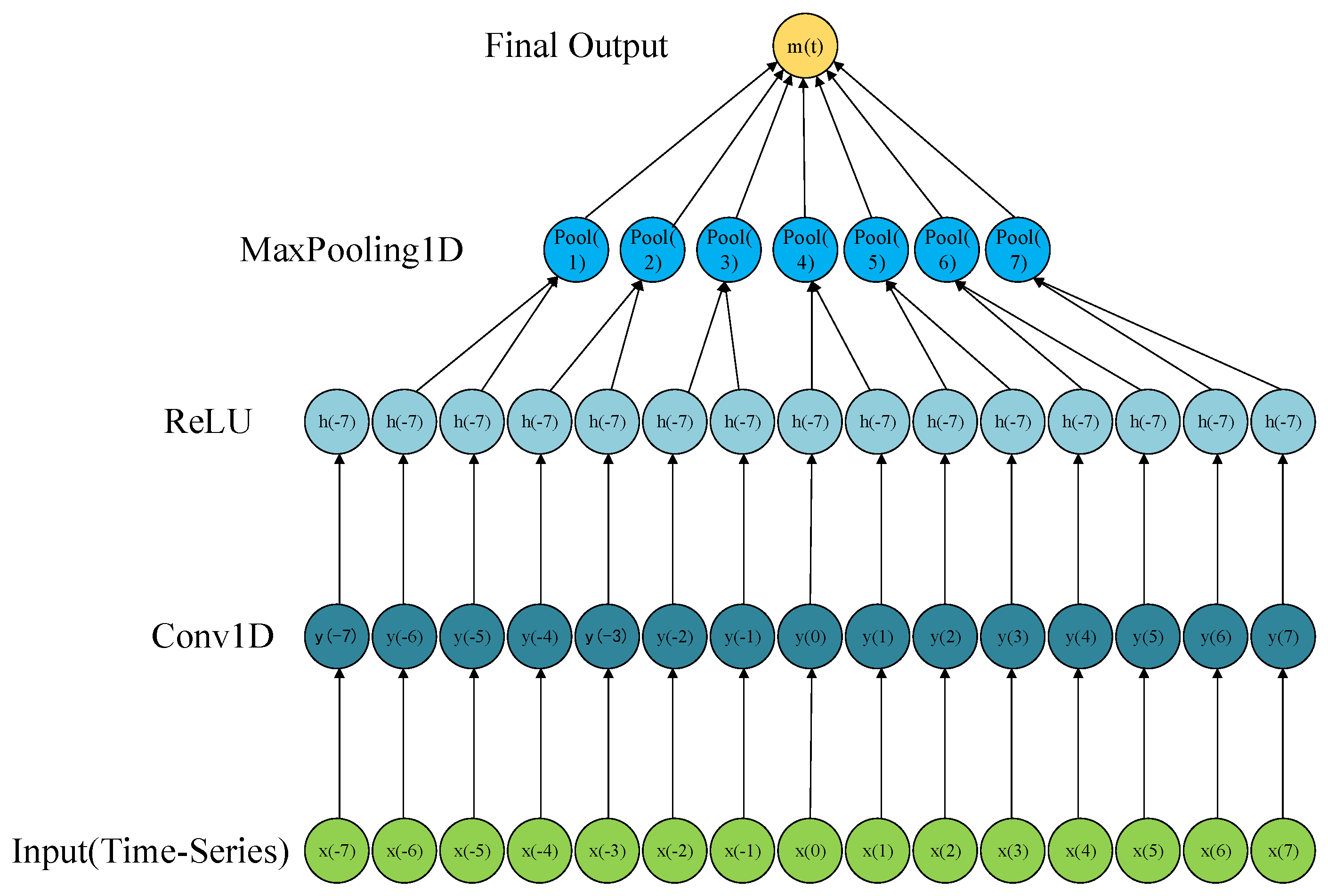
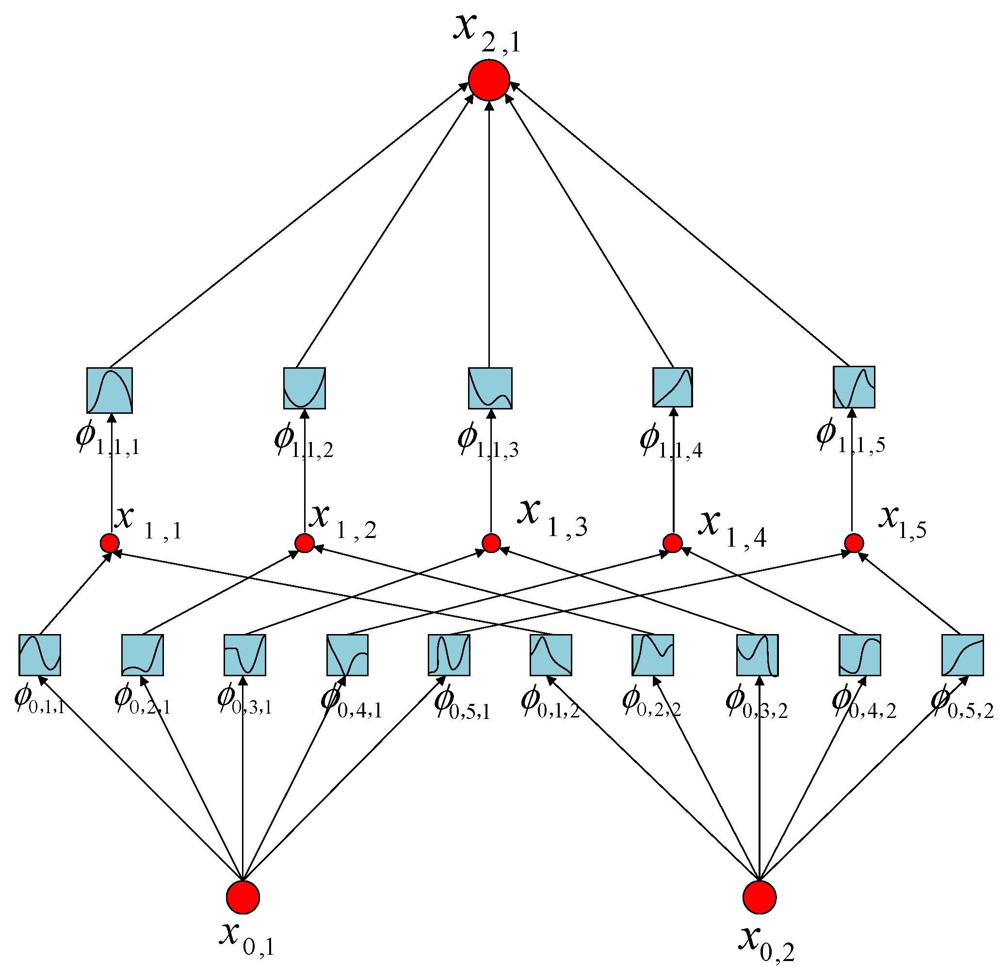
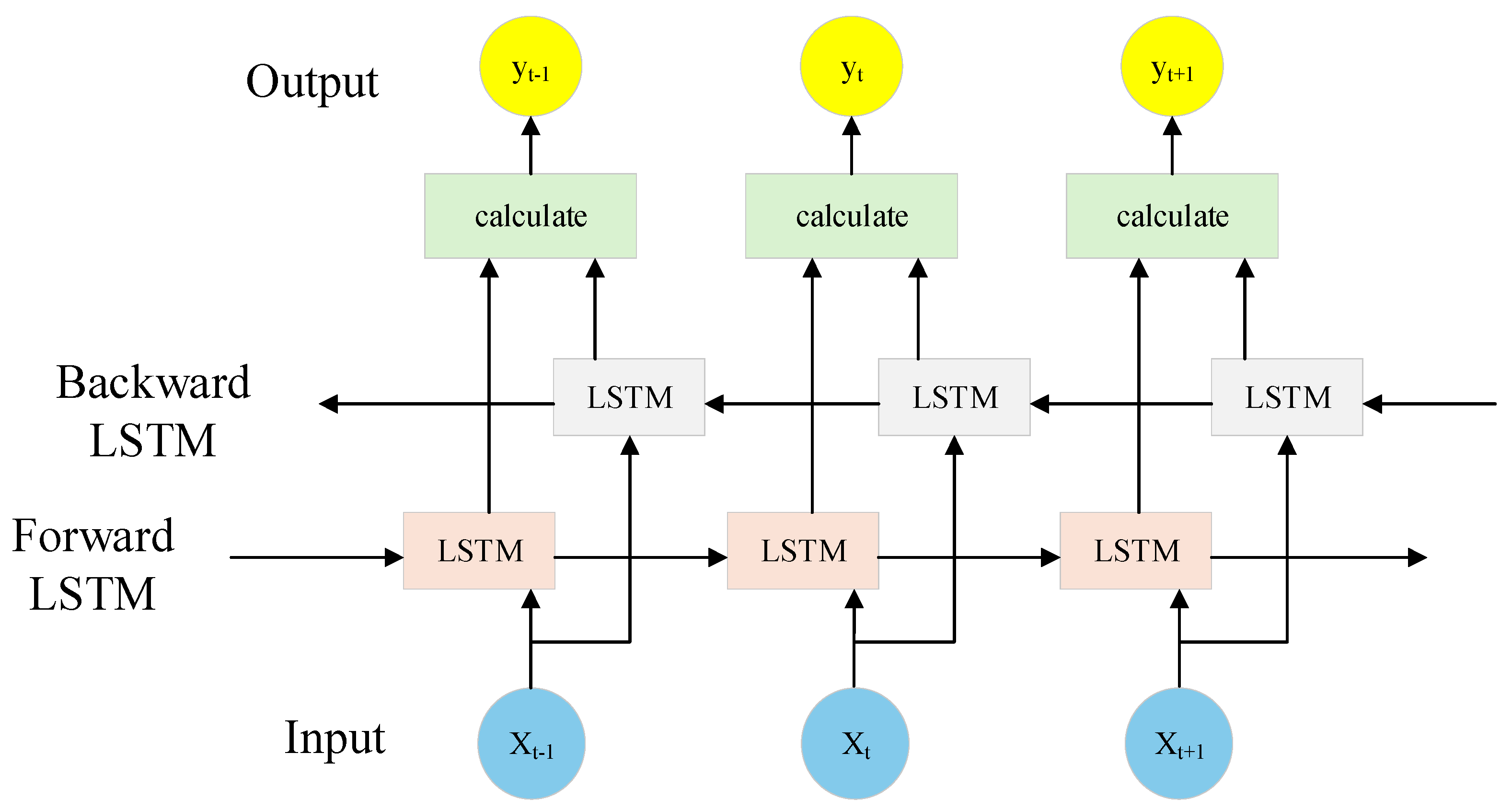
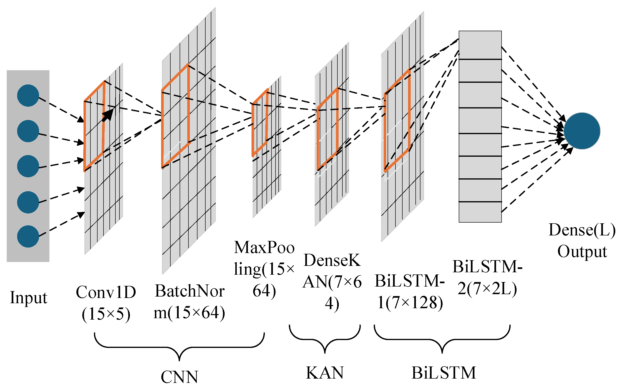
To overcome the above problems, this paper proposes the CNN-KAN-BiLSTM hybrid deep learning model. Among them, KAN is a deep learning method based on the Kolmogorov–Arnold approximation theorem. By utilizing B-Spline basis functions for feature transformation, KAN can effectively approximate complex nonlinear relationship. By integrating the advantages of convolutional feature extraction, nonlinear transformation enhancement and bidirectional time series modeling, the accuracy and robustness of SOH estimation are improved. This model first uses CNN to extract the local patterns of the input features, then adopts the Kolmogorov–Arnold Network (KAN) to replace the traditional fully connected layer to enhance the nonlinear mapping ability. Finally, the temporal evolution law of SOH is learned from both the positive and negative directions through the BiLSTM module to enhance the model’s ability to capture the degradation trend of batteries. Compared with the traditional hybrid structure, CNN-KAN-BiLSTM has achieved key improvements in multiple aspects. First, in terms of estimation accuracy, the KAN layer has adaptive activation ability, which can fit more complex nonlinear relationships and effectively improve the estimation accuracy. Second, in terms of computational complexity, the KAN module has a compact structure and is highly efficient in training without significantly increasing the computational burden of the overall model. Third, in terms of interpretability, the construction form of KAN makes the mapping process of intermediate features more physically readable, which is helpful for analyzing the specific influence of different features on SOH. Fourth, in terms of robustness, BiLSTM can capture temporal features from both forward and reverse directions, enhancing the model’s ability to adapt to inconsistent battery data and noise disturbances. Therefore, CNN-KAN-BiLSTM not only structurally optimizes the deficiencies of the existing models in terms of function expression, generalization ability, and interpretability, but also provides a more forward-looking solution for complex SOH modeling problems.

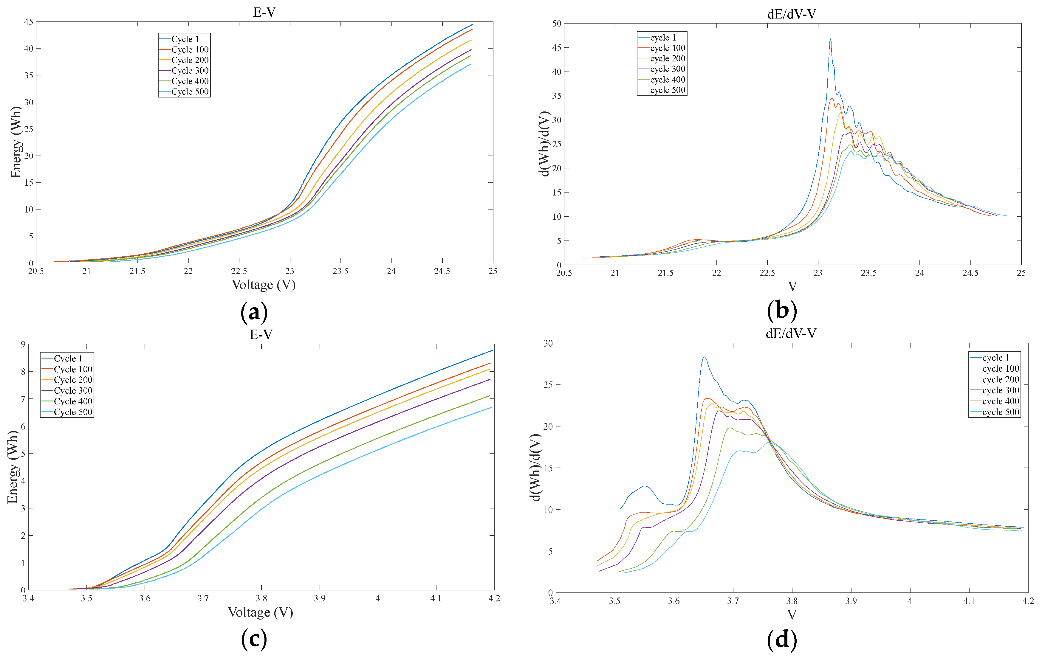
In this paper, a novel SOH estimation framework for hybrid models is proposed. First, incremental energy analysis (IEA) is proposed. Based on the measured charging data of lithium batteries, the incremental energy (IE) curve is plotted according to the voltage-energy relationship. The SOH of lithium batteries is characterized using the features extracted from the IE curve. Compared to ICA, IEA accounts for energy loss and provides a more comprehensive description of the battery aging process. Subsequently, a CNN-KAN-BiLSTM deep learning model is proposed. CNN provides basic local structural information, KAN performs nonlinear reconstruction of features and enhances the response of key variables, and BiLSTM [38] further integrates time-dependent information. This approach enables accurate modeling and stable estimation of SOH variation trends. The main contributions of this paper are summarized as follows:

(1)

Based on the data of the lithium battery charging stage, this paper constructs a multi-feature sequence integrating IE features and temperature features, and introduces voltage mean variance (VVM) and temperature mean standard deviation (SDTM) to characterize the internal inconsistencies of the battery pack. This sequence retains the multi-dimensional feature structure of each period and constitutes a time series in a cyclic order, which more effectively reflects the evolution trend of SOH over time and significantly improves the prediction accuracy and robustness of the model.

(2)

This paper proposes the CNN-KAN-BiLSTM model for accurately estimating the SOH of batteries, integrating local feature extraction, nonlinear modeling and temporal trend perception. Experiments were conducted under different working conditions covering battery pack and single cells with multiple charging rates. The characteristics of incremental energy and incremental capacity were compared respectively, as well as models such as CNN-KAN, CNN-LSTM, KAN, and BiLSTM. The results show that the proposed model achieves the optimal performance on all datasets, with MAE < 0.4%, RMSE < 0.5%, and R² > 97%, fully verifying its accuracy, stability and generalization ability.

(3)

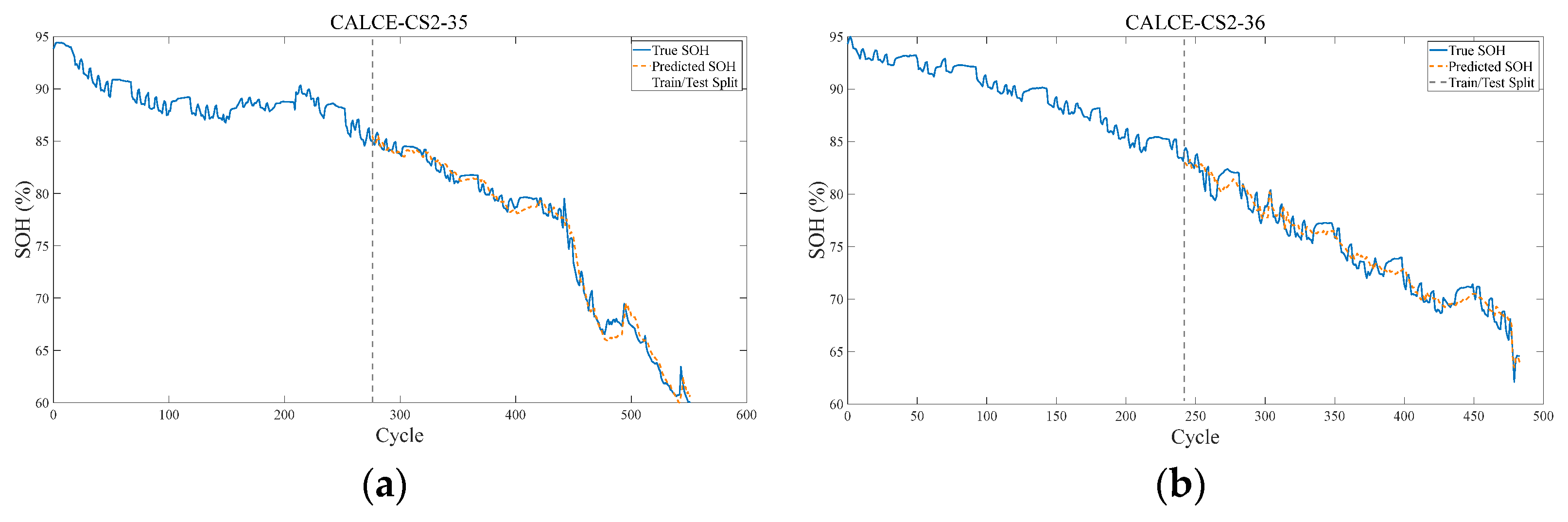
In this paper, experimental verification was carried out using public datasets. This paper also experimentally verified the SOH estimation method proposed in this study by using the NASA battery dataset and the CALCE battery dataset. The experimental results show that in the face of public battery datasets from different sources and with various working conditions, this method demonstrates strong robustness and generalization ability in terms of SOH estimation accuracy, curve smoothness, and the ability to fit the degradation trend, further verifying the adaptability and practical value of the proposed model in multiple scenarios.

2. Feature Extraction and Correlation Analysis

2.1. Incremental Energy Curve

The energy increment curve (dE/dV-V) represents the rate of energy change during the battery discharge process, and its shape evolves with battery aging. Compared to the battery’s voltage or capacity, the IE curve more intuitively shows the variation in battery power during cycling. Changes in the standard deviation and mean of the IE curve can indicate issues, such as increased internal resistance and polarization. Therefore, using the characteristics of the IE curve can more effectively capture the nonlinear changes associated with battery aging. The calculation formula for IE is shown in Equation (2):

$$IE={\displaystyle \frac{dE}{dV}}={\displaystyle \frac{E_{i+1}-E_i}{V_{i+1}-V_i}}$$

(2)

where IE represents the derivative of the incremental energy concerning the voltage, i.e., the rate of change of the energy to the voltage. $E_i$ denotes the accumulated energy at the i-th sampling point, and $V_i$ indicates the voltage at the i-th sampling point. ${\displaystyle \frac{dE}{dV}}$ quantifies the energy increment per unit voltage change, which is essentially the derivative of energy with respect to voltage and can also be interpreted as a measure of the average power output capacity within the voltage range.

The incremental energy (IE) curve is derived from the first-order differentiation of the original E-V curve. The IE curve is smoother, which reduces measurement errors and improves estimation accuracy. Additionally, it maintains good stability under different operating conditions, effectively enhancing the model’s generalization capability. Figure 1a–d illustrates the E-V and IE curves of aging datasets for a lithium battery pack and a 0.5 C battery cell across different cycles.

As shown in Figure 1, subfigures (a) and (c) respectively present the E-V curves of the battery pack and the 0.5 C single cell. The numbers in the legend represent different cycle times. With the advancement of the cycle, the E-V curves of both gradually shift downward as a whole, and the cumulative energy value per unit voltage decreases, reflecting the trend of gradual attenuation of battery capacity. Meanwhile, in the E-V curve of the battery pack shown in Figure 1a, the originally obvious voltage platform gradually Narrows and slows down within the range of 22.5 V to 24.5 V. This phenomenon is also reflected in the range of 3.6 V to 3.9 V of the 0.5 C single cell shown in Figure 1c. This indicates that the main reaction range of the battery is deteriorating, and the electrode reaction kinetics is weakening.

To reveal these change processes more clearly, this paper further performs first-order differentiation on the E-V curve to obtain the incremental energy (IE) curve. The IE curves of the corresponding battery pack and 0.5 C single cell are shown in subgraphs (b) and (d) of Figure 1, respectively. It can be seen that as the number of cycles increases, the height of the main peak of the IE curve decreases significantly, the voltage corresponding to the peak gradually shifts to the right, and the area under the curve also continues to shrink. These changes are due to factors such as the loss of active substances and the irreversible loss of lithium ions, which cause an increase in internal resistance, thereby reducing the energy release efficiency of the battery and gradually “collapsing” the voltage platform. Therefore, the characteristics such as peak amplitude, peak position drift, and area shrinkage in the IE curve are highly consistent with phenomena such as weakened energy distribution and degradation of the voltage platform in the E-V curve. They can depict the degradation process of battery performance from multiple dimensions and provide reliable characteristic support for the evaluation of battery SOH.

2.1.1. Feature Extraction Based on Incremental Energy Curve

The peak value of the IE curve typically indicates the maximum energy release capacity or reaction capacity of the battery during charging and discharging. With the increase in battery use time, internal aging mechanisms such as the growth of the SEI film and electrolyte consumption lead to a decrease in its maximum energy release capacity. Using the peak value as a feature to estimate SOH directly reflects the battery’s health. The formula for calculating the peak value is shown in Equation (3):

$${IE}_{Peak}=\max (E)$$

(3)

where E is the incremental energy of the battery during each charge–discharge cycle, representing the energy output capacity of the battery. The peak value represents the maximum energy output during the cycle.

To comprehensively analyze the intensity of the chemical reaction inside the battery using the IE curve, the average value of the IE curve is introduced. The formula for calculating the average value is presented in Equation (4):

$$\mu ={\displaystyle \frac{1}{N}}{\displaystyle \sum _{i=1}^N{E}_i}$$

(4)

where $\mu$ is the average of the incremental energy, indicating the average energy release of the battery over a specific period; $E_i$ is the incremental energy value in each charge-discharge cycle; and $N$ is the total number of cycles.

The standard deviation indicates the decline in battery consistency. As the battery ages, the performance of its internal cells becomes increasingly inconsistent, resulting in greater fluctuations in overall battery performance. The formula for calculating the standard deviation is shown in Equation (5):

$$\sigma =\sqrt{{\displaystyle \frac{1}{N}}{\displaystyle \sum _{t=1}^N{(E_t-\mu )}^2}}$$

(5)

where $\sigma$ is the standard deviation, indicating the degree of fluctuation in the battery’s performance; $E_t$ is the incremental energy value in each charge-discharge cycle, representing the energy change of the battery per cycle; $\mu$ is the average incremental energy, representing the average energy output level over all cycles; and $N$ is the total number of data points, corresponding to the number of measured cycles.

The area of the incremental energy curve represents the total energy within a specific voltage interval. When the battery SOH drops, the area under the IE curve tends to decrease. This reduction can be directly related to capacity decay and thus used for SOH estimation. Its calculation formula is shown in Equation (6):

$$A={\displaystyle {\int }_{V_{min}}^{V_{max}}\frac{dE}{dV}}dV$$

(6)

where A is the total integral area, representing the integral value of the entire incremental energy curve.

2.1.2. Inconsistent Characteristics of Lithium Battery Pack

The correlation between the area characteristics of the battery pack’s incremental energy curve and SOH has been weak. Based on the operating characteristics of series battery pack, voltage mean variance (VVM) is proposed as an alternative feature to characterize the inconsistency of battery pack. By calculating the dispersion degree between the voltage mean variance of each cell, the inconsistency of series batteries can be quantified effectively. Considering that battery aging often results in significant voltage differences between cells, this feature can provide key dynamic information for SOH estimation. Its calculation formula is shown in Equation (7):

$$\phi ={\displaystyle \frac{1}{N}}{\displaystyle \sum _{i=1}^N{(V_i-{\mu }_V)}^2}$$

(7)

where $V_i$ is the voltage value of the i-th battery in the battery pack, ${\mu }_V$ is the average voltage of all cells in the battery pack, and $N$ is the number of batteries or channels. In this experiment, there are 6 battery channels.

2.2. Temperature Characteristic

Temperature affects both the charge-discharge characteristics of the battery and directly accelerates its aging process. Therefore, introducing temperature characteristics is essential to enhancing the accuracy and stability of SOH estimation.

Considering that the temperature inconsistency of the battery pack is mainly characterized by temperature fluctuation, with the fluctuation amplitude negatively correlated to the uniformity of temperature distribution, it can be quantitatively characterized through standard deviation calculations. An increase in the standard deviation of the mean temperature typically indicates intensified system inconsistency, which may negatively impact the accuracy of SOH assessments. Therefore, the standard deviation of temperature means (SDTM) is adopted as the temperature characteristic of the battery pack. The data processing procedure in this experiment is divided into two stages. First, the six-channel temperature data from each sampling point is averaged arithmetically. Then, the standard deviation of the mean temperature across all sampling points in the cycle is calculated as shown in Equation (8):

$${\sigma }_T=\sqrt{{\displaystyle \frac{1}{N}}{\displaystyle \sum _{j=1}^N{(T_{mean,j}-{\mu }_T)}^2}}$$

(8)

where $N$ is the total number of sampling points in the cycle, ${\mu }_T$ is the average temperature of all sampling points in the cycle, and ${\sigma }_T$ is the standard deviation of the mean temperature in the cycle.

For the battery cell, this paper uses the average temperature of each aging cycle as the temperature characteristic input. The formula for calculating the average temperature is shown in Equation (9):

$$T_{avg}={\displaystyle \frac{1}{N}}{\displaystyle \sum _{i=1}^N{T}_i}$$

(9)

where $T_i$ is the temperature sampling value of the battery in a specific cycle, and $N$ is the number of sampling points.

2.3. Correlation Analysis

The Pearson correlation coefficient (PCC), typically represented by the symbol r, is a statistical index that measures the degree of linear correlation between two variables. Its value ranges from -1 to 1. When the value is close to ±1, it indicates a high correlation; when the value is close to 0, it indicates almost no correlation. The formula for calculating the Pearson correlation coefficient is shown in Equation (10):

$$r={\displaystyle \frac{{\displaystyle \sum (X_i-\overline{X})}(Y_i-\overline{Y})}{\sqrt{{\displaystyle \sum {(X_i-\overline{X})}^2}}\cdot \sqrt{{\displaystyle \sum {(Y_i-\overline{Y})}^2}}}}$$

(10)

where $X_i$ and $Y_i$ represent two variables in the dataset (e.g., feature and SOH), and $\overline{X}$ and $\overline{Y}$ represent the mean of X and Y, respectively.

The Pearson correlation coefficients between the extracted features and the battery SOH are calculated. The corresponding results for the battery pack are shown in

Table 1. Correlation coefficients between each feature of the battery pack and the SOH of the battery.

Feature	Peak Value	Mean Value	Standard Deviation	Voltage Mean Variance
Correlation coefficient	0.899	0.932	0.917	−0.951

. Taking the battery cell with a 0.5 C charging rate as an example, the corresponding results are shown in

Table 2. Correlation coefficients between each feature of the IE curve and the SOH of the battery cell (0.5 C).

Feature	Peak Value	Mean Value	Standard Deviation	Area
Correlation coefficient	0.993	0.998	0.988	0.999

.

The data in the tables indicate that the Pearson correlation coefficients between the proposed features (for both battery pack and cells) and the battery SOH are close to 1. This suggests a strong correlation between the features and cell SOH, justifying their selection for SOH estimation.

3. Construction of CNN-KAN-BiLSTM Model

3.1. The Structure, Principle and Application of CNN

Convolutional Neural Networks (CNNs) are deep learning models designed for processing grid-structured data, such as images and time series. In this paper, CNNs are primarily used to extract local features from incremental energy curves and temperature data. The battery aging process is reflected in local changes in voltage, energy, and temperature; thus, CNNs can effectively capture these subtle patterns through convolutional kernels. Specifically, the one-dimensional convolution layer performs sliding window calculations on input multi-feature sequences, such as peaks, averages, standard deviations, etc., to extract local correlations. As shown in Figure 2, the convolutional architecture of the neural network includes an input layer, a one-dimensional convolutional layer, an activation function layer, a pooling layer, and an output layer.

(1)

1D convolution layer.

The formula for the convolution operation is shown in Equation (11):

$$y_t^{(K)}={\displaystyle \sum _{i=0}^{M-1}{x}_{t+i}}{W}_t^{(K)}+b^{(K)}$$

(11)

where $y_t^{\left(k\right)}$ is the output value of the convolution kernel $k$ at time step $t$, $x_{t+i}$ is the value of the input time series, $W_i^{\left(k\right)}$ is the weight of the convolution kernel (size $M$), $b^{\left(k\right)}$ is the bias term, and $M$ is the convolution window size (i.e., the length of the convolution kernel).

(2)

Activation Function Layer (ReLU).

The ReLU definition is shown in Equation (12):

$$h_t^{(k)}=\max (0,y_t^{(k)})$$

(12)

where $y_t^{\left(k\right)}$ is the output of the convolution layer, and $h_t^{\left(k\right)}$ is the value after ReLU activation.

(3)

Pooled horizon.

The maximum pooling operation is shown in Equation (13):

$$\mathrm{pool}(t)=\max (h_t,h_{t+1},\dots ,h_{t+M-1})$$

(13)

where $M$ is the pool window size, and $h_t$ is the eigenvalue after ReLU processing.

The output layer of a CNN is usually a dense layer that integrates the local features extracted after convolution, activation, and pooling operations, mapping them to the target output dimension. The output layer converts the local features extracted by the CNN into high-dimensional representations, which serve as input for the subsequent KAN network.

3.2. The Structure, Principle and Application of KAN

Kolmogorov–Arnold Networks (KANs) are a new type of neural network based on the Kolmogorov–Arnold representation theorem. This theorem states that if f is a multivariate continuous function defined on a bounded domain, then the smooth function f: [0, 1]ⁿ→R can be expressed in the form of Equation (14):

$$f(x_1,x_2,\dots ,x_n)={\displaystyle \sum _{q=1}^{2n+1}{\mathsf{\Phi }}_q}\left({\displaystyle \sum _{p=1}^n{\lambda }_{qp}}{x}_p\right)$$

(14)

where ${\lambda }_{pq}$: ${[0,1]}^n$→R, and ${\mathsf{\Phi }}_q$: R→R. This means that, mathematically, any multivariate function can be constructed from univariate functions through addition operations. This provides a theoretical basis for KAN’s design and inspires its approach of transforming multivariate function learning into the learning of multiple univariate functions.

This theory serves as an effective tool for solving high-dimensional data problems. In battery systems, data is often high-dimensional, and SOH estimation involves complex nonlinear relationships. Through its nonlinear activation and linear combination characteristics, KAN can effectively reduce data dimensionality and improve modeling efficiency.

This paper innovatively proposes replacing the traditional fully connected layer with KAN to enhance the nonlinear expression ability. Unlike the standard fully connected layers that rely on fixed activation functions, KAN achieves adaptive nonlinear transformation by introducing trainable basis functions at each neuron, enabling the model to fit the complex mapping relationship between input features and output in a more flexible way. In the estimation of battery SOH, the degradation process often has high nonlinearity and diversity. Introducing KAN as the feature transformation module helps to improve the expressive ability and fitting accuracy of the model, especially showing stronger generalization performance in capturing weak degradation trends and handling cross-sample differences. KAN is primarily used for the nonlinear transformation and optimization of local features extracted by CNN, enabling a more accurate depiction of the complex relationship between battery SOH and input features. Specifically, KAN’s feature transformation layer uses B-Spline basis functions to map input features, such as IE curve peaks or temperature averages into a high-dimensional space, forming new feature representations. These new features more effectively characterize the nonlinear behavior of battery aging. Subsequently, the linear combination layer integrates these transformed features, further enhancing the model’s feature representation capability. KAN primarily consists of a feature transformation layer, a B-Spline calculation layer, a linear combination layer, and a final output layer. The KAN structure is shown in Figure 3.

(1)

Feature transform layer.

Each input feature $x_p$ undergoes a set of univariate transformations (represented by B-Splines) and is mapped to a high-dimensional feature space, as shown in Equation (15):

$${\tilde{x}}_{p,q}={\varphi }_{p,q}(x_p)$$

(15)

where $x_p$ represents the input feature, ${\varphi }_{p,q}\left(x_p\right)$ denotes the nonlinear transformation function calculated by B-Splines, and ${\tilde{x}}_{p,q}$ represents the new feature after transformation.

(2)

B-Spline computing layer.

Each univariate transformation ϕ(x) is calculated using B-Splines. The mathematical expression is shown in Equation (16):

$${\varphi }_{p,q}(x)={\displaystyle \sum _{i=0}^n{c}_i}{B}_{i,k}(x)$$

(16)

where $B_{i,k}\left(x\right)$ is the B-Spline basis function, and its formula is shown in Equations (17) and (18).

$$B_{i,0}(x)=\left\{\begin{array}{ll}1,\hfill & t_i\le x<t_{i+1}\hfill \\ 0,\hfill & otherwise\hfill \end{array}\right.$$

(17)

$$B_{i,k}(x)={\displaystyle \frac{x-t_i}{t_{i+k}-t_i}}{B}_{i,k-1}(x)+{\displaystyle \frac{t_{i+k+1}-x}{t_{i+k+1}-t_{i+1}}}{B}_{i+1,k-1}(x)$$

(18)

(3)

Linear composite layer.

Features transformed by B-Splines are further linearly weighted, as shown in Equation (19):

$$x_{l,k}={\displaystyle \sum _j{\lambda }_{l,k,j}}{\tilde{x}}_j$$

(19)

where $x_{l,k}$ is the final output feature of the KAN layer and serves as input to the BiLSTM layer, ${\lambda }_{l,k,j}$ is a trainable weight parameter, and ${\tilde{x}}_j$ is the j-th feature transformed by the B-Spline basis function.

(4)

Final output layer.

$$y={\displaystyle \sum _q{w}_q}{\varphi }_q(x)$$

(20)

where $w_q$ is the trainable feature weight, and ${\varphi }_q\left(x\right)$ is the feature from the B-Spline.

3.3. The Structure, Principle and Application of BiLSTM

Long Short-Term Memory (LSTM) is an improved recurrent neural network (RNN) specifically designed to address long-term dependency problems, making it suitable for processing time series data. This paper adopts the bidirectional long short-term memory (BiLSTM) neural network, a variant of LSTM, that introduces a bidirectional propagation mechanism alongside standard LSTM. BiLSTM processes time series data in both forward and backward directions simultaneously, enhancing its ability to capture temporal dependencies.

This paper innovatively introduces BiLSTM as the output layer to model the timing characteristics of SOH. BiLSTM is introduced as the output layer of the model to more comprehensively model the temporal dependence of battery SOH evolution with the cycling process. Although the traditional unidirectional LSTM can capture the forward dependencies in the sequence, during the battery degradation process, the change of SOH is often jointly affected by multiple cyclic states before and after. BiLSTM enhances the model’s ability to understand the complete temporal context by simultaneously integrating the forward and reverse temporal information of the sequence, thereby improving the perception and prediction accuracy of the SOH degradation trend. In addition, the BiLSTM structure helps alleviate the problem of long-term dependence and enhances the model’s robustness and generalization ability when dealing with different individual batteries and operating conditions. The input to BiLSTM consists of a feature sequence processed by CNN and KAN. The forward LSTM captures the battery’s degradation trend from early to current cycles, while the backward LSTM analyzes historical data from the current cycle to identify potential capacity recovery or mutation points. This bidirectional modeling capability enables the model to estimate SOH more accurately, particularly when battery capacity fluctuates or self-healing occurs, while maintaining stable estimation performance. The calculation formulas are shown in Equations (21), (22), and (23):

$$h_t^{\mathrm{forward}}=\mathrm{LSTM}(x_t,h_{t-1}^{\mathrm{forward}})$$

(21)

$$h_t^{\mathrm{backward}}=\mathrm{LSTM}(x_t,h_{t+1}^{\mathrm{backward}})$$

(22)

$$h_t=[h_t^{\mathrm{forward}},h_t^{\mathrm{backward}}]$$

(23)

where $x_t$ represents the output of the KAN layer (i.e., higher-order temporal features), $h_t^{forward}$ denotes the hidden state at the last time step of the forward LSTM (transmitting historical degradation trends), and $h_t^{backward}$ denotes the hidden state at the next time step of the backward LSTM (learning abnormal patterns from future data in reverse). $h_t$ represents the concatenation of the forward and backward hidden states. Since BiLSTM shares the $x_t$ output from KAN, the fused $h_t$ integrates local features extracted by the CNN, nonlinear transformations from the KAN layer, and bidirectional temporal dependencies. While $h_t^{forward}$ captures the overall slope decline, $h_t^{backward}$ identifies step-like edge points, resulting in a smooth and accurate final $h_t$ output. The BiLSTM structure diagram is shown in Figure 4.

In the CNN-KAN-BiLSTM deep learning model proposed in this paper, each network layer has a distinct role and operates synergistically. The CNN layer extracts local spatial structure information from input features, enhancing the model’s sensitivity to key patterns. The KAN layer utilizes powerful nonlinear function approximation capabilities to connect feature extraction with temporal modeling. The BiLSTM layer fully leverages bidirectional dependencies of features over time, thereby improving the modeling of battery SOH evolution trends. The overall architecture achieves efficient fusion from spatial feature extraction to nonlinear mapping and then to temporal modeling, significantly enhancing the model’s ability to represent and process complex features while outperforming traditional single-structure models.

Figure 5 shows the structural diagram of the CNN-KAN-BiLSTM deep learning model developed in this paper:

4. Experimental Procedure, Results, and Analysis

4.1. Experimental Data

The experimental data were obtained from aging tests of a lithium battery pack measured in the laboratory as well as from three battery cells tested under different charging rates (0.1 C, 0.2 C, and 0.5 C). The materials used in the experiment are Lishen 18650 lithium batteries, each with a nominal capacity of 2.5 Ah and a voltage of 3.6 V, respectively. The lithium battery pack consists of six series-connected lithium-ion battery cells with identical specifications. Aging tests of the battery pack and individual cells were conducted at room temperature using a Neware high-performance battery test system built in the laboratory, and the aging data of the lithium battery pack and each cell were measured. The testing system comprises a battery cell testing device, a battery pack testing device, and a host computer, all characterized by high responsiveness and precision.

The aging test of the battery pack begins by charging at a constant current of 1.2 A until the end voltage of the battery pack reaches the cut-off voltage of 24.9 V. Next, the lithium battery pack is charged at a constant voltage of 24.9 V until the current drops to 68 mA, at which point the charging is stopped. Subsequently, a constant discharge is carried out at 2.4 A until the battery terminal voltage drops to 19.3 V. The experiment is terminated when the maximum discharge capacity of the battery pack reaches the failure threshold, which is approximately 65% of the rated capacity. The battery cell (0.5 C) is charged at a constant current of 1.25 A until the battery terminal voltage reaches the cut-off voltage of 4.2 V. It is then charged at a constant voltage of 4.2 V until the current drops to 48 mA, at which point the charging is stopped. Finally, a constant discharge is carried out at 1.25 A until the battery terminal voltage drops to 3 V. The experiment is terminated when the maximum discharge capacity of the single battery reaches the failure threshold, which is about 80% of the rated capacity.

4.2. Experimental Procedure

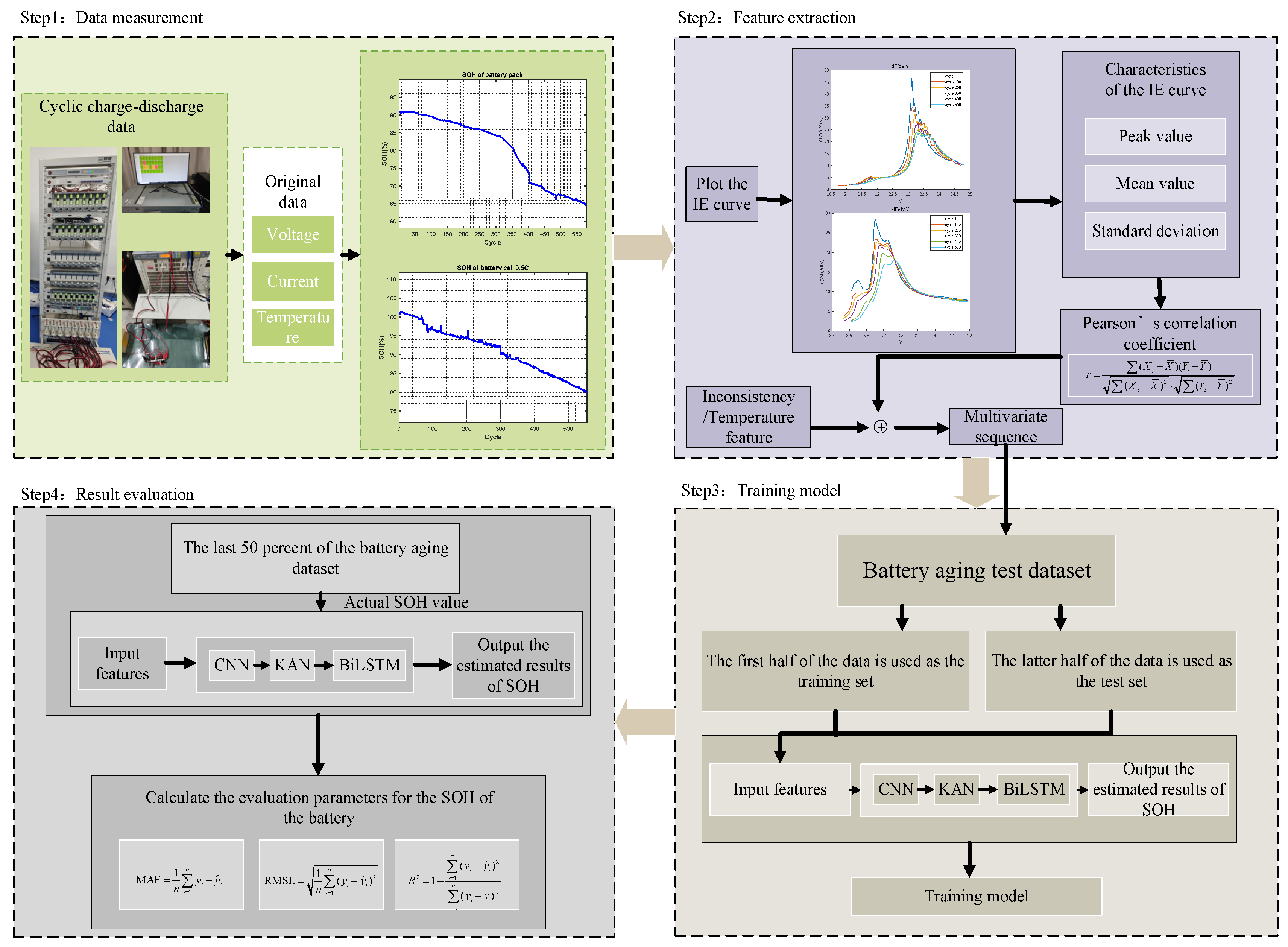
This experiment primarily involved SOH estimation for a lithium battery pack and battery cells with varying charging rates. The specific experimental steps are shown in Figure 6 and described as follows:

Step 1.

The raw data, such as current, voltage, energy, and temperature of the battery pack and individual were measured and calculated using the experimental equipment during the charging stage.

Step 2.

Based on the recorded energy, voltage and temperature data, the incremental energy (IE) curves of the battery pack and each cell were plotted respectively, and the relevant features, such as peak value, average value, and standard deviation, were extracted. Meanwhile, statistical features, such as average temperature and temperature variance, were extracted from the temperature data to jointly construct a multi-feature sequence integrating energy-temperature information. Subsequently, the Pearson correlation coefficient was used to evaluate the correlations between the above-mentioned various characteristics and the SOH of battery pack and cells to verify its effectiveness in SOH modeling.

Step 3.

The processed datasets were divided into training and test sets. The extracted features were input into the CNN-KAN-BiLSTM deep learning model for training. The results of the battery SOH estimation were estimated, and evaluation metrics, MAE, RMSE, and R² were calculated for subsequent performance analysis.

4.3. Experimental Results and Analysis

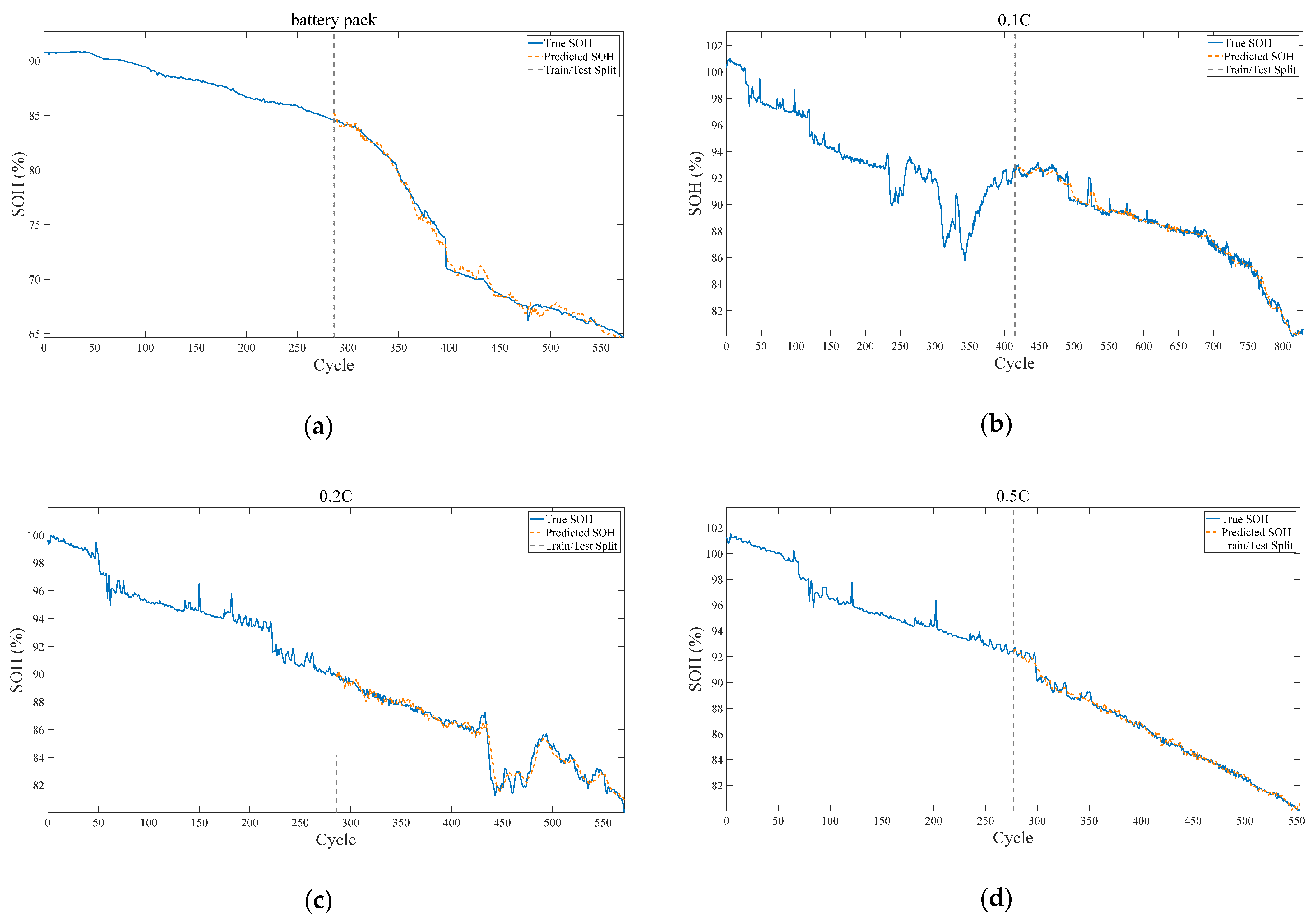
Figure 7 shows the SOH of a battery pack and three individual battery cells at different charging rates, plotted as a function of the number of cycles. The figure demonstrates that the SOH values for both the battery pack and each cell generally exhibit a downward trend with increasing cycles, however, this decline is not smooth. SOH fluctuations may occur due to temperature effects. Following each charge–discharge cycle, the battery is typically rested for some time, during which electrode polarization may partially recover, leading to brief capacity increases.

It is worth noting that in the Figure 7b,d, the SOH curves of the two batteries in the early cycling stage are slightly above 100%. This is mainly attributed to the common slight capacity increase phenomenon in the initial cycle of lithium-ion batteries, that is, the released effective capacity briefly exceeds the nominal capacity. According to the SOH calculation method adopted in this paper, that is, the ratio of the maximum measured discharge capacity to the nominal capacity, a calculation result with SOH slightly exceeding 100% will occur. This phenomenon does not reflect abnormal battery performance, but is caused by the structural activation process of the graphite anode material during the initial cycle, including microscopic changes such as the expansion of interlayer spacing and the shedding of particles into nanosheets, which cause it to release more effective lithium intercalation sites and enhance reversible capacity. This capacity “rebound” process is more significant under conditions such as high temperature or depth of discharge (DOD) [43]. If the battery manufacturing process is uniform and the initial activation of the negative electrode material is sufficient (such as moderate compaction and good wetting of the electrolyte), its initial state may be close to the theoretical capacity upper limit. In the subsequent cycle, due to the limited space for structural activation, the phenomenon of SOH exceeding 100% may not be significantly manifested, as shown in the battery in Figure 7c. It should be pointed out that a SOH slightly above 100% is an acceptable technical phenomenon in practical applications and will not have a substantial impact on the judgment of the SOH change trend or the validity of model evaluation.

To rigorously evaluate the accuracy of SOH estimation, the performance of the regression model was assessed using common metrics: MAE, RMSE, and R². Their definitions are provided in Equations (24), (25), and (26), respectively:

$$\mathrm{MAE}={\displaystyle \frac{1}{n}}{\displaystyle \sum _{i=1}^n|}{y}_i-{\widehat{y}}_i|$$

(24)

$$\mathrm{RMSE}=\sqrt{{\displaystyle \frac{1}{n}}{\displaystyle \sum _{i=1}^n{(y_i-{\widehat{y}}_i)}^2}}$$

(25)

$$R^2=1-{\displaystyle \frac{{\displaystyle \sum _{i=1}^n{(y_i-{\widehat{y}}_i)}^2}}{{\displaystyle \sum _{i=1}^n{(y_i-\overline{y})}^2}}}$$

(26)

where $n$ is the number of charge-discharge cycles, $y_i$ indicates the true SOH, $\overline{y}$ is the average true SOH, and ${\widehat{y}}_i$ is the estimated SOH. Smaller MAE and RMSE values indicate higher model accuracy, while R² closer to 1 indicates better model fit. The experimental results are shown in Figure 8:

The figure shows the SOH estimation results of the proposed model for lithium batteries across four different working conditions. It includes data from a battery pack (Figure 7a) and three groups of battery cells charged at varying rates (0.1 C, 0.2 C, and 0.5 C; Figure 7b–d). The estimated SOH curves closely align with the actual SOH curves, demonstrating strong fitting accuracy under all working conditions. The estimated trends are highly consistent with the real degradation processes, highlighting the model’s excellent generalization capability. Under the condition where the SOH degradation of the lithium battery pack and the 0.5 C battery cell is relatively stable, the estimated curve closely matches the true value, indicating the model’s strong capability in capturing overall degradation trends. For the 0.1 C and 0.2 C cells which exhibit fluctuating SOH, the model effectively identifies key change points without significant deviation in noisy environments, demonstrating its good stability.

The CNN-KAN-BiLSTM deep learning model effectively integrates the advantages of each layer. The CNN layer extracts local change patterns from input features, enhancing the ability to perceive and capture micro-features related to degradation behavior. The KAN layer performs nonlinear modeling on the features extracted by CNN, mapping them into a space that better describes the degradation process. Compared to traditional models, KAN exhibits a stronger nonlinear representation capability while maintaining interpretability. The BiLSTM layer accepts the KAN output, generates state representations at each time step, and ultimately estimates SOH. This architecture leverages the strengths of each layer, forming a closed-loop system that achieves effective SOH estimation. As shown in

Table 3. SOH assessment results.

Battery Testing	MAE (%)	RMSE (%)	R2 (%)
Battery pack	0.3910	0.4797	99.46
0.1 C	0.2728	0.3792	98.76
0.2 C	0.3301	0.4494	97.07
0.5 C	0.2094	0.2699	99.37

, MAE across all working conditions is below 0.4%, R² exceeds 97%, and the R² for the lithium battery pack reaches as high as 99.46%. These results indicate that this model not only has excellent performance and efficiency but also demonstrates strong adaptability to the actual complex and variable real-world data.

To further verify the feasibility and effectiveness of the proposed SOH estimation method for lithium batteries, this paper presents a feature comparison experiment alongside four deep learning model comparison experiments. Specifically, the feature comparison experiment involved extracting features from the incremental capacity (IC) curve, including peak value, average value, standard deviation, and area, while incorporating battery temperature characteristics to form a comprehensive multi-feature sequence. These features were then compared with those proposed in this paper, and the respective sequences were input into the deep learning model for training to assess the estimation performance of both methods on battery SOH. The model comparison experiment tested CNN-KAN, CNN-LSTM, KAN, and BiLSTM models using identical input features to compare their SOH estimation effectiveness. The results of the feature comparison experiment are presented in Figure 9.

The evaluation parameters for the SOH estimation in the feature comparison experiment are shown in

Table 4. Evaluation results of comparative characteristics of batteries under various working conditions.

Working Condition	Feature Type	MAE (%)	RMSE (%)	R2 (%)
Battery Pack	IEA	0.3910	0.4797	99.46
	ICA	0.7568	0.9800	97.78
0.1 C	IEA	0.2728	0.3792	98.76
	ICA	0.6555	0.9258	92.65
0.2 C	IEA	0.3301	0.4494	97.07
	ICA	0.6780	0.9091	88.02
0.5 C	IEA	0.2094	0.2699	99.37
	ICA	0.6701	0.8255	94.10

.

The comparison of SOH estimation curves in Figure 8 clearly illustrates the impact of the two feature types on model performance. Assessment results based on IEA features are generally smoother, demonstrating better fitting accuracy and improved detection of key change points during abrupt SOH changes and fluctuation phases. This indicates that IEA features effectively enhance model adaptability and stability under nonlinear and complex conditions.

By comparing SOH estimation results based on incremental capacity (ICA) and incremental energy (IEA) features across various working conditions, the superiority of IEA becomes evident. For the battery pack, the MAE with IEA (0.3910%) is significantly lower than with ICA (0.7568%). RMSE decreases from 0.9800% (ICA) to 0.4798% (IEA), while R² increases from 97.78% to 99.47%. Similar trends are observed for 0.1 C, 0.2 C, and 0.5 C cells, highlighting IEA’s effectiveness in capturing battery aging behavior and energy degradation trends.

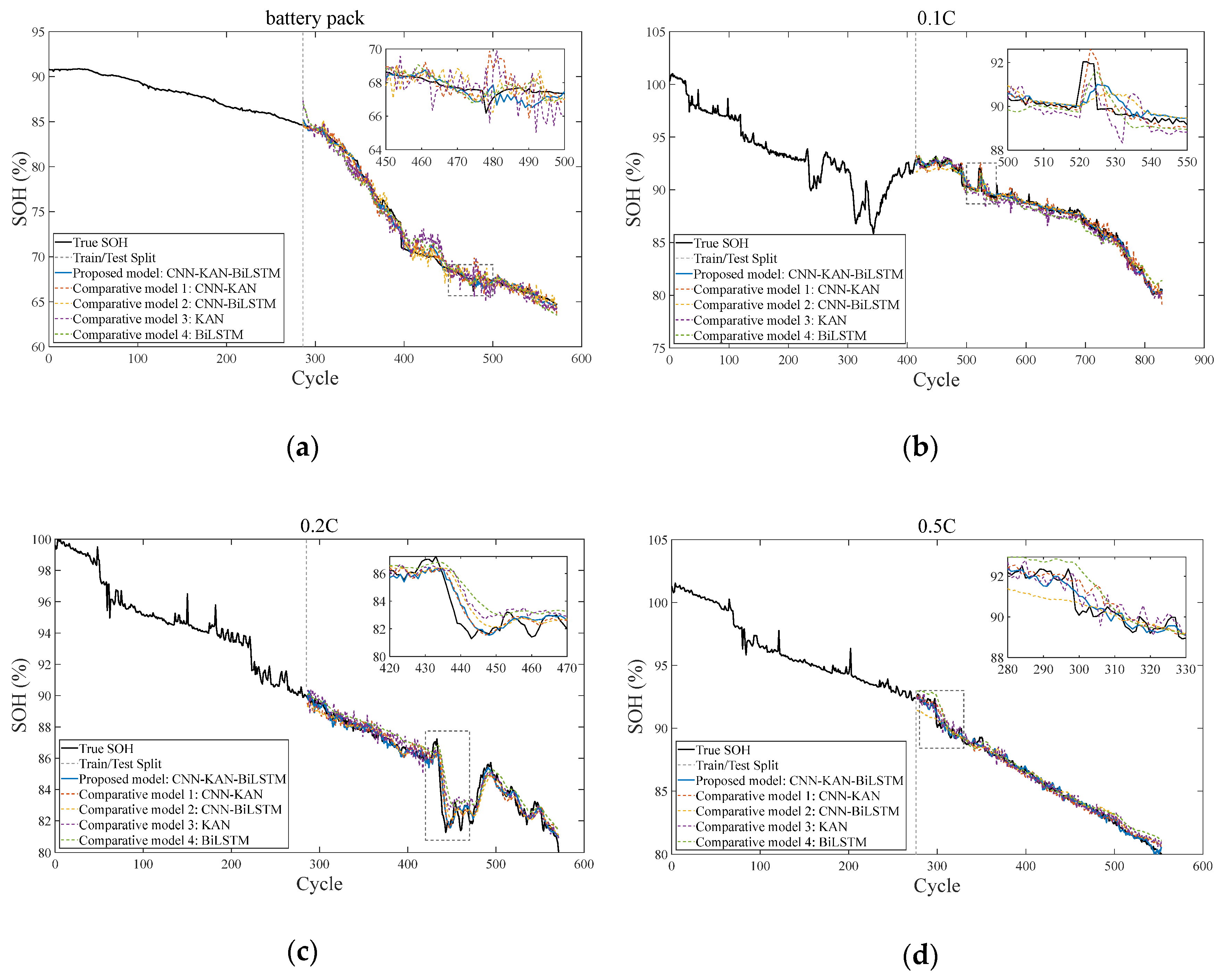
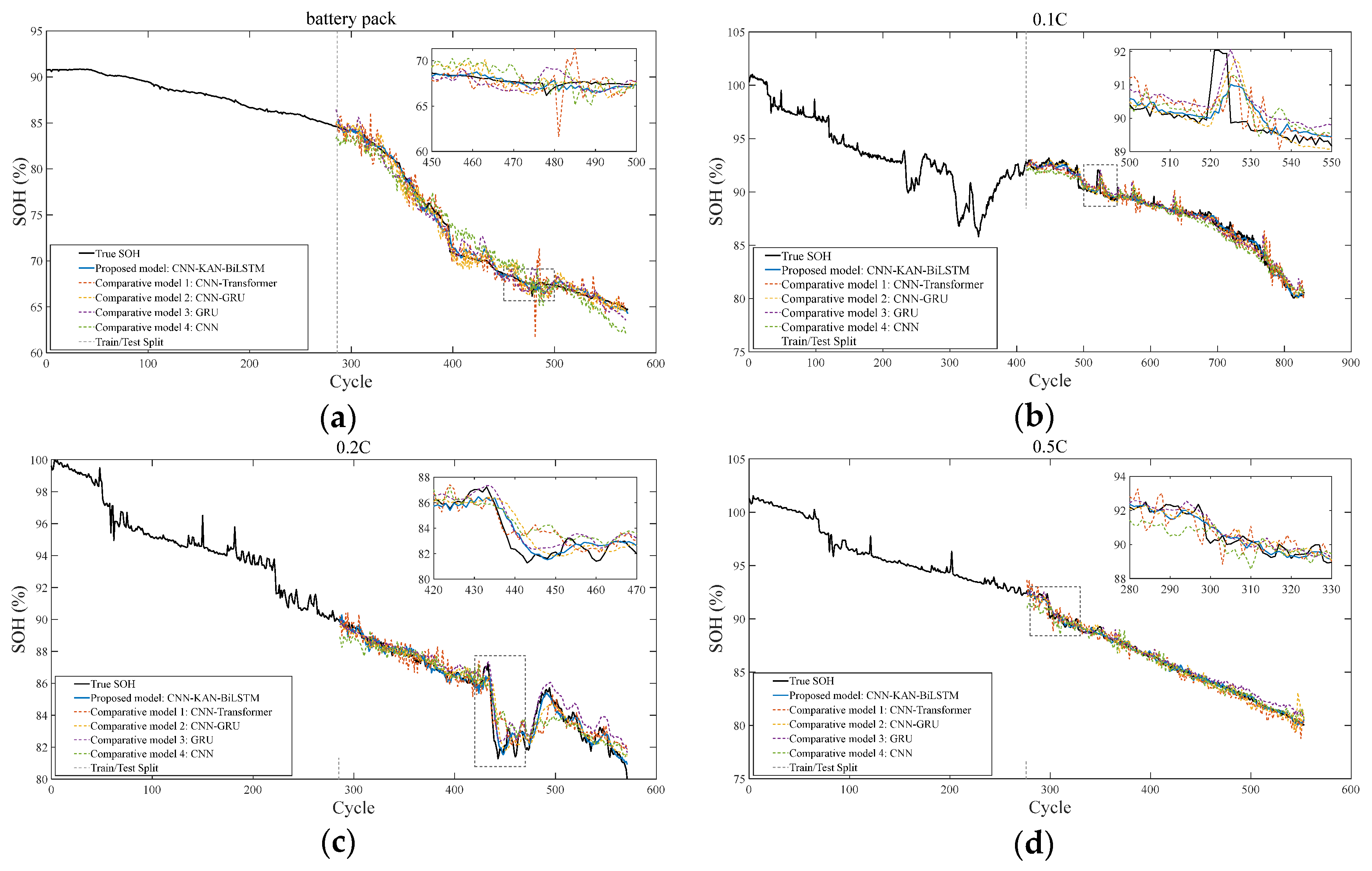
The model comparison results are displayed in Figure 10.

The final evaluation metrics of the proposed model and the four compared models are provided in

Table 5. The evaluation results of each model based on IEA characteristics on battery pack.

Model	MAE (%)	RMSE (%)	R2 (%)
CNN-KAN-BiLSTM	0.3910	0.4797	99.46
CNN-KAN	0.5251	0.6999	98.86
CNN-BiLSTM	0.4802	0.6309	99.08
KAN	0.8671	1.0998	97.19
BiLSTM	0.7196	0.8994	98.12

,

Table 6. The evaluation results of each model based on IEA characteristics on battery cell (0.1 C).

Model	MAE (%)	RMSE (%)	R2 (%)
CNN-KAN-BiLSTM	0.2728	0.3792	98.76
CNN-KAN	0.3206	0.4497	98.27
CNN-BiLSTM	0.3693	0.4980	97.87
KAN	0.4293	0.5308	97.51
BiLSTM	0.5058	0.6031	96.79

,

Table 7. The evaluation results of each model based on IEA characteristics on battery cell (0.2 C).

Model	MAE (%)	RMSE (%)	R2 (%)
CNN-KAN-BiLSTM	0.3301	0.4494	97.07
CNN-KAN	0.3999	0.5000	96.38
CNN-BiLSTM	0.4332	0.5996	94.79
KAN	0.4798	0.6830	92.58
BiLSTM	0.6251	0.8193	89.32

and

Table 8. The evaluation results of each model based on IEA characteristics on battery cell (0.5 C).

Model	MAE (%)	RMSE (%)	R2 (%)
CNN-KAN-BiLSTM	0.2094	0.2699	99.37
CNN-KAN	0.3012	0.3989	98.62
CNN-BiLSTM	0.3674	0.4779	98.02
KAN	0.3314	0.4104	98.30
BiLSTM	0.4180	0.5606	97.28

.

By observing the SOH estimation effects of the aforementioned models under various working conditions, it is evident that the models demonstrate good estimation performance. However, the proposed CNN-KAN-BiLSTM model achieves highly consistent fitting with the real SOH curve across all conditions. When the degradation curve exhibits abrupt changes and jitter, the model maintains stable outputs. Although the CNN-KAN model effectively extracts local features and performs nonlinear mapping, its lack of temporal modeling results in slight deficiencies in capturing long-term SOH degradation trends. The CNN-LSTM model captures temporal dependencies but lacks KAN’s nonlinear feature optimization, leading to lower accuracy in complex working conditions. When used alone, the BiLSTM model fails to extract local incremental energy features, resulting in poor overall performance. The CNN-KAN model outperforms CNN-LSTM in short-term SOH estimation due to its nonlinear mapping of CNN-extracted features; however, its long-term estimation errors increase without temporal modeling. The CNN-LSTM model is suitable for long-term estimation, but gradient vanishing during drastic SOH changes reduces its accuracy. Conversely, the KAN model relies solely on nonlinear mapping and lacks feature extraction and temporal modeling capabilities, leading to poor performance. The proposed CNN-KAN-BiLSTM model performs exceptionally in estimating the lithium-ion battery SOH. By comparing real and estimated SOH values, the model accurately captures degradation trends with minimal errors, indicating its strong capability to learn SOH variations. The RMSE and MAE of the CNN-KAN-BiLSTM model are significantly lower than those of other models, demonstrating higher accuracy and reduced errors.

Analysis reveals that the proposed model maintains high accuracy across various battery conditions, especially during nonlinear SOH degradation. The CNN-KAN-BiLSTM model utilizes CNN for local feature extraction, KAN for nonlinear transformation, and BiLSTM for handling temporal dependency, effectively learning SOH patterns and improving generalization. Consequently, this method improves both the accuracy and stability of lithium-ion battery SOH estimation, providing a reliable solution for intelligent monitoring.

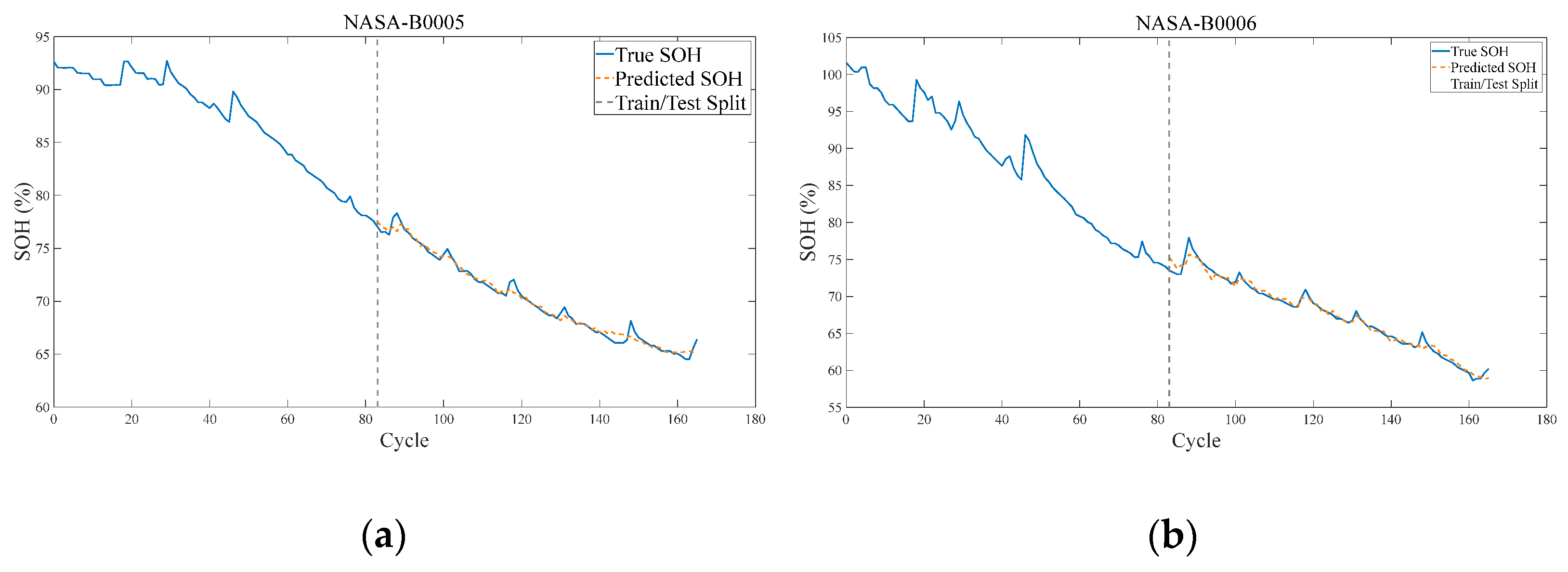
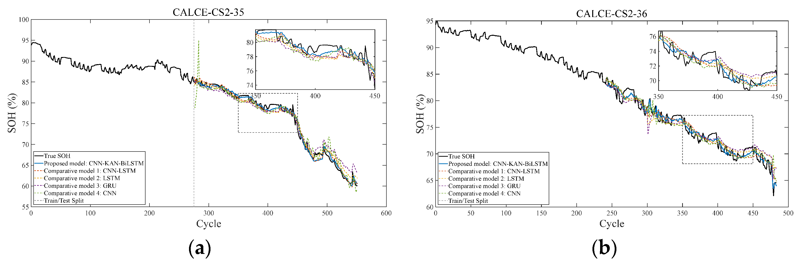
In addition, this paper also incorporates comparative evaluation experiments of some existing models, and the experimental results are shown in Figure 11.

The final evaluation indicators of the comparative experiments of some existing models are shown in

Table 9. The evaluation results of the existing benchmark models based on IEA characteristics on battery pack.

Model	MAE (%)	RMSE (%)	R2 (%)
CNN-KAN-BiLSTM	0.3910	0.4797	99.46
CNN-Transformer	0.6926	0.9560	97.88
CNN-GRU	0.6841	0.8595	98.29
GRU	0.7502	0.8996	98.13
CNN	1.1967	1.4446	95.17

,

Table 10. The evaluation results of the existing benchmark models based on IEA characteristics on battery cell (0.1 C).

Model	MAE (%)	RMSE (%)	R2 (%)
CNN-KAN-BiLSTM	0.2728	0.3792	98.76
CNN-Transformer	0.5118	0.6547	96.32
CNN-GRU	0.4171	0.5911	97.00
GRU	0.4411	0.5588	97.32
CNN	0.5509	0.6802	96.03

,

Table 11. The evaluation results of the existing benchmark models based on IEA characteristics on battery cell (0.2 C).

Model	MAE (%)	RMSE (%)	R2 (%)
CNN-KAN-BiLSTM	0.3301	0.4494	97.07
CNN-Transformer	0.5845	0.7772	91.24
CNN-GRU	0.4268	0.6198	94.43
GRU	0.5515	0.6823	93.25
CNN	0.6215	0.8295	90.02

and

Table 12. The evaluation results of the existing benchmark models based on IEA characteristics on battery cell (0.5 C).

Model	MAE (%)	RMSE (%)	R2 (%)
CNN-KAN-BiLSTM	0.2094	0.2699	99.37
CNN-Transformer	0.4412	0.5606	97.28
CNN-GRU	0.3402	0.4698	98.09
GRU	0.3820	0.4804	98.00
CNN	0.3941	0.5349	97.52

.

5. Validation of Public Datasets

5.1. NASA Battery Dataset

To verify the effectiveness of the proposed SOH estimation method, this paper selects the B0005 and B0006 lithium-ion battery datasets provided by NASA for experiments. This dataset contains real working condition data, complete charge and discharge cycle information, and rich sensor parameters. It is widely used in the research of battery health status assessment and life prediction, and can provide a reliable basis for model training and verification. The experimental results are shown in Figure 12a,b.

The final evaluation indicators obtained through experiments using the NASA dataset are shown in

Table 13. The final evaluation results of NASA’s batteries.

Battery Type	MAE (%)	RMSE (%)	R2 (%)
B0005	0.3548	0.4867	98.46
B0006	0.4767	0.6604	98.09

.

In order to verify the validity and universality of the method proposed in this paper, namely the SOH estimation method based on the characteristics of IE curves. This paper also conducts experiments based on the benchmark model. The experimental results are shown in Figure 13.

The final evaluation indicators of each model experiment are shown in

Table 14. Experimental evaluation indicators based on the benchmark model. (NASA-B0005).

Model	MAE (%)	RMSE (%)	R2 (%)
CNN-KAN-BiLSTM	0.3548	0.4867	98.46
CNN-LSTM	0.5064	0.6894	96.91
LSTM	0.5723	0.7291	96.54
GRU	0.6946	0.8000	95.84
CNN	0.6702	0.8695	95.08

and

Table 15. Experimental evaluation indicators based on the benchmark model. (NASA-B0006).

Model	MAE (%)	RMSE (%)	R2 (%)
CNN-KAN-BiLSTM	0.4767	0.6604	98.09
CNN-LSTM	0.5362	0.7298	97.66
LSTM	0.6425	0.8391	96.91
GRU	0.7326	0.8987	96.46
CNN	0.8393	1.0498	95.16

.

5.2. CALCE Battery Dataset

In this paper, the CS2-35 and CS2-36 lithium-ion battery datasets provided by the CALCE Center of the University of Maryland were also selected for experimental verification. This dataset features standardized charge and discharge protocols, complete cycle data, and rich sensor parameters. It is widely used in battery health status assessment and life prediction research, providing a reliable basis for model training and validation. The experimental results are shown in Figure 14 and Figure 15.

The final evaluation indicators obtained through experiments using the CALCE dataset are shown in

Table 16. The final evaluation results of CALCE’s batteries.

Battery Type	MAE (%)	RMSE (%)	R2 (%)
CS2-35	0.6689	0.8239	98.91
CS2-36	0.8497	0.9852	95.94

.

The results of the experiments based on the benchmark model are shown in Figure 15.

The final evaluation indicators of each model experiment are shown in

Table 17. Experimental evaluation indicators based on the benchmark model. (CALCE-CS2-35).

Model	MAE (%)	RMSE (%)	R2 (%)
CNN-KAN-BiLSTM	0.6689	0.8239	98.91
CNN-LSTM	0.8177	1.0100	98.36
LSTM	0.9126	1.1098	98.02
GRU	1.3120	1.5969	95.90
CNN	1.1284	1.5876	95.94

and

Table 18. Experimental evaluation indicators based on the benchmark model. (CALCE-CS2-36).

Model	MAE (%)	RMSE (%)	R2 (%)
CNN-KAN-BiLSTM	0.8497	0.9852	95.94
CNN-LSTM	1.0242	1.2154	93.83
LSTM	1.1718	1.4668	91.01
GRU	1.1551	1.4673	91.00
CNN	1.0986	1.3828	92.01

.

6. Conclusions

In this paper, a method for SOH estimation of lithium-ion batteries based on incremental energy characteristics and CNN-KAN-BiLSTM is proposed. Key features are extracted from the incremental energy curve, which incorporates specific inconsistencies of the battery pack, while temperature features are combined to form an effective set of input features. The CNN-KAN-BiLSTM model is trained to achieve high-precision SOH estimation. The experimental results show that this method effectively estimates the SOH of the battery. The feasibility and superiority of this method are confirmed by comparative experiments. Both the RMSE and MAE are below 1%, demonstrating excellent performance.

Although the CNN-KAN-BiLSTM model proposed in this paper shows good prediction accuracy and generalization ability in the battery SOH estimation task, there are still certain limitations. First, the current model has not yet introduced the self-attention mechanism. Therefore, when dealing with high-dimensional features or complex working conditions, it may have insufficient responses to key features, limiting its adaptability to multiple types of batteries and variable working conditions. Second, the experiment only constructed features and conducted modeling based on the data from the charging stage. Although the charging stage has the advantages of strong stability and high data quality, it ignored the characteristic information during the discharging process, which might lead to the model having an insufficient understanding of the battery’s state changes throughout its life cycle. In addition, this paper mainly conducts experimental verification based on laboratory data and partial data from the two public datasets of NASA and CALCE. Although it is somewhat representative, there is still a gap compared with the actual operating environment of energy storage power stations or new energy vehicles. The stability and practicality of the model under real complex working conditions still need to be further tested. Therefore, future research can consider introducing the self-attention mechanism to enhance the recognition ability of key features. At the same time, it integrates the full-cycle data of charging and discharging, and combines the real vehicle and power station operation data in actual application scenarios to construct an SOH estimation model that is closer to the real working conditions.

Future work could introduce a self-attention mechanism to enhance the model’s focus on critical features, enabling adaptation to diverse battery types and working conditions. This improvement would enhance generalization capability and estimation accuracy, ultimately supporting the intelligent management of new energy vehicles and energy storage systems. Additionally, integrating operational data from energy storage power stations with measurement data from new energy vehicles could build a SOH estimation model that is more aligned with real-world applications. Large-scale, multi-cycle data from power stations can reveal long-term battery degradation patterns, while real vehicle data reflect dynamic characteristics under complex conditions. Combining these data sources would enhance model adaptability in practical environments and advance SOH estimation technology toward engineering applications and intelligence.

References

1. Demirci, O.; Taskin, S.; Schaltz, E.; Demirci, B.A. Review of battery state estimation methods for electric vehicles—Part II: SOH estimation. J. Energy Storage 2024, 96, 112703. [Google Scholar] [CrossRef]
2. Vignesh, S.; Che, H.S.; Selvaraj, J.; Tey, K.S.; Lee, J.W.; Shareef, H.; Errouissi, R. State of health (SoH) estimation methods for second life lithium-ion battery—Review and challenges. Appl. Energy 2024, 369, 123542. [Google Scholar]
3. Peng, S.; Wang, Y.; Tang, A.; Jiang, Y.; Kan, J.; Pecht, M. State of Health Estimation Joint Improved Grey Wolf Optimization Algorithm and LSTM Using Partial Discharging Health Features for Lithium-Ion Batteries. Energy 2025, 315, 134293. [Google Scholar] [CrossRef]
4. Liu, Y.; Wang, L.; Li, D.; Wang, K. State-of-health estimation of lithium-ion batteries based on electrochemical impedance spectroscopy: A review. Prot. Control Mod. Power Syst. 2023, 8, 41. [Google Scholar] [CrossRef]
5. Li, X.; Lyu, M.; Li, K.; Gao, X.; Liu, C.; Zhang, Z. Lithium-ion battery state of health estimation based on multi-source health indicators extraction and sparse Bayesian learning. Energy 2023, 282, 128445. [Google Scholar] [CrossRef]
6. Zhang, C.; Luo, L.; Yang, Z.; Zhao, S.; He, Y.; Wang, X.; Wang, H. Flexible method for estimating the state of health of lithium-ion batteries using partial charging segments. Energy 2024, 295, 131009. [Google Scholar] [CrossRef]
7. Zhang, C.; Tu, L.; Yang, Z.; Du, B.; Zhou, Z.; Wu, J.; Chen, L. A CMMOG-based lithium-battery SOH estimation method using multi-task learning framework. J. Energy Storage 2025, 107, 114884. [Google Scholar] [CrossRef]
8. Zhang, S.; Guo, X.; Dou, X.; Zhang, X. A rapid online calculation method for state of health of lithium-ion battery based on coulomb counting method and differential voltage analysis. J. Power Sources 2020, 479, 228740. [Google Scholar] [CrossRef]
9. Bian, X.; Wei, Z.; Li, W.; Pou, J.; Sauer, D.U.; Liu, L. State-of-health estimation of lithium-ion batteries by fusing an open circuit voltage model and incremental capacity analysis. IEEE Trans. Power Electron. 2021, 37, 2226–2236. [Google Scholar] [CrossRef]
10. Obregon, J.; Han, Y.R.; Ho, C.W.; Mouraliraman, D.; Lee, C.W.; Jung, J.Y. Convolutional autoencoder-based SOH estimation of lithium-ion batteries using electrochemical impedance spectroscopy. J. Energy Storage 2023, 60, 106680. [Google Scholar] [CrossRef]
11. Pang, Z.; Yang, K.; Song, Z.; Niu, P.; Chen, G.; Meng, J. A new method for determining SOH of lithium batteries using the real-part ratio of EIS specific frequency impedance. J. Energy Storage 2023, 72, 108693. [Google Scholar] [CrossRef]
12. Jiang, B.; Zhu, J.; Wang, X.; Wei, X.; Shang, W.; Dai, H. A comparative study of different features extracted from electrochemical impedance spectroscopy in state of health estimation for lithium-ion batteries. Appl. Energy 2022, 322, 119502. [Google Scholar] [CrossRef]
13. Peng, S.; Zhang, D.; Dai, G.; Wang, L.; Jiang, Y.; Zhou, F. State of charge estimation for LiFePO4 batteries joint by PID observer and improved EKF in various OCV ranges. Appl. Energy 2025, 377, 124435. [Google Scholar] [CrossRef]
14. Li, K.; Wang, Y.; Chen, Z. A comparative study of battery state-of-health estimation based on empirical mode decomposition and neural network. J. Energy Storage 2022, 54, 105333. [Google Scholar] [CrossRef]
15. Chen, L.; Xie, S.; Lopes, A.M.; Li, H.; Bao, X.; Zhang, C.; Li, P. A new SOH estimation method for lithium-ion batteries based on model-data-fusion. Energy 2024, 286, 129597. [Google Scholar] [CrossRef]
16. Li, C.; Yang, L.; Li, Q.; Zhang, Q.; Zhou, Z.; Meng, Y.; Zhao, X.; Wang, L.; Zhang, S.; Li, Y.; et al. SOH estimation method for lithium-ion batteries based on an improved equivalent circuit model via electrochemical impedance spectroscopy. J. Energy Storage 2024, 86, 111167. [Google Scholar] [CrossRef]
17. Xiang, H.; Wang, Y.; Li, K.; Zhang, X.; Chen, Z. A comprehensive study on state-of-charge and state-of-health estimation of sodium-ion batteries. J. Energy Storage 2023, 72, 108314. [Google Scholar] [CrossRef]
18. Liu, C.; Deng, Z.; Zhang, X.; Bao, H.; Cheng, D. Battery state of health estimation across electrochemistry and working conditions based on domain adaptation. Energy 2024, 297, 131294. [Google Scholar] [CrossRef]
19. Xiong, R.; Sun, Y.; Wang, C.; Tian, J.; Chen, X.; Li, H.; Zhang, Q. A data-driven method for extracting aging features to accurately predict the battery health. Energy Storage Mater. 2023, 57, 460–470. [Google Scholar] [CrossRef]
20. Deng, Z.; Hu, X.; Li, P.; Lin, X.; Bian, X. Data-driven battery state of health estimation based on random partial charging data. IEEE Trans. Power Electron. 2022, 37, 5021–5031. [Google Scholar] [CrossRef]
21. Lin, M.; Yan, C.; Wang, W.; Dong, G.; Meng, J.; Wu, J. A data-driven approach for estimating state-of-health of lithium-ion batteries considering internal resistance. Energy 2023, 277, 127675. [Google Scholar] [CrossRef]
22. Qian, G.; Zheng, Y.; Li, X.; Sun, Y.; Han, X.; Ouyang, M. State of health estimation for lithium-ion batteries using impedance-based simplified timescale information. Appl. Energy 2025, 382, 125272. [Google Scholar] [CrossRef]
23. Li, X.; Yuan, C.; Wang, Z.; Xie, J. A data-fusion framework for lithium battery health condition estimation based on differential thermal voltammetry. Energy 2022, 239, 122206. [Google Scholar] [CrossRef]
24. Chen, C.; Xiong, R.; Yang, R.; Li, H. A novel data-driven method for mining battery open-circuit voltage characterization. Green Energy Intell. Transp. 2022, 1, 100001. [Google Scholar] [CrossRef]
25. Rahimian, S.K.; Tang, Y. A practical data-driven battery state-of-health estimation for electric vehicles. IEEE Trans. Ind. Electron. 2023, 70, 1973–1982. [Google Scholar] [CrossRef]
26. Tang, A.; Xu, Y.; Hu, Y.; Tian, J.; Nie, Y.; Yan, F.; Tan, Y.; Yu, Q. Battery state of health estimation under dynamic operations with physics-driven deep learning. Appl. Energy 2024, 370, 123632. [Google Scholar] [CrossRef]
27. Wu, T.; Huang, Y.; Xu, Y.; Jiang, J.; Liu, S.; Li, Z. SOH prediction for lithium-ion battery based on improved support vector regression. Int. J. Green Energy 2023, 20, 227–236. [Google Scholar] [CrossRef]
28. Yang, N.; Song, Z.; Hofmann, H.; Sun, J. Robust state of health estimation of lithium-ion batteries using convolutional neural network and random forest. J. Energy Storage 2022, 48, 103857. [Google Scholar] [CrossRef]
29. Wang, X.; Hu, B.; Su, X.; Xu, L.; Zhu, D. State of health estimation for lithium-ion batteries using random forest and gated recurrent unit. J. Energy Storage 2024, 76, 109796. [Google Scholar] [CrossRef]
30. Lu, J.; Xiong, R.; Tian, J.; Wang, C.; Sun, F. Deep learning to estimate lithium-ion battery state of health without additional degradation experiments. Nat. Commun. 2023, 14, 2760. [Google Scholar] [CrossRef]
31. Che, Y.; Deng, Z.; Li, P.; Tang, X.; Khosravinia, K.; Lin, X.; Hu, X. State of health prognostics for series battery packs: A universal deep learning method. Energy 2022, 238, 121857. [Google Scholar] [CrossRef]
32. Bao, X.; Chen, L.; Lopes, A.M.; Li, X.; Xie, S.; Li, P.; Chen, Y. Hybrid deep neural network with dimension attention for state-of-health estimation of lithium-ion batteries. Energy 2023, 278, 127734. [Google Scholar] [CrossRef]
33. Tang, A.; Wu, X.; Xu, T.; Hu, Y.; Long, S.; Yu, Q. State of health estimation based on inconsistent evolution for lithium-ion battery module. Energy 2024, 286, 129575. [Google Scholar] [CrossRef]
34. Ma, Y.; Shan, C.; Gao, J.; Chen, H. A novel method for state of health estimation of lithium-ion batteries based on improved LSTM and health indicators extraction. Energy 2022, 251, 123973. [Google Scholar] [CrossRef]
35. He, Y.; Deng, Z.; Chen, J.; Li, W.; Zhou, J.; Xiang, F.; Hu, X. State-of-health estimation for fast-charging lithium-ion batteries based on a short charge curve using graph convolutional and long short-term memory networks. J. Energy Chem. 2024, 98, 1–11. [Google Scholar] [CrossRef]
36. Shu, X.; Chen, Z.; Shen, J.; Ye, M.; Zhang, Q.; Liu, Y.; Liu, X.; Hu, Y. Robust state of health estimation for lithium-ion batteries considering random charging behaviors. IEEE Trans. Transp. Electrif. 2025, 11, 5545–5554. [Google Scholar] [CrossRef]
37. Zhang, C.; Luo, L.; Yang, Z.; Zhao, S.; He, Y.; Wang, X.; Wang, H. Battery SOH estimation method based on gradual decreasing current, double correlation analysis and GRU. Green Energy Intell. Transp. 2023, 2, 100108. [Google Scholar] [CrossRef]
38. Zhao, J.; Han, X.; Ouyang, M.; Burke, A.F. Specialized deep neural networks for battery health prognostics: Opportunities and challenges. J. Energy Chem. 2023, 87, 416–438. [Google Scholar] [CrossRef]
39. Li, Z.; Zhang, X.; Gao, W. State of health estimation of lithium-ion battery during fast charging process based on BiLSTM-Transformer. Energy 2024, 311, 133418. [Google Scholar] [CrossRef]
40. Xiong, X.; Wang, Y.; Jiang, C.; Zhang, X.; Xiang, H.; Chen, Z. End-to-end deep learning powered battery state of health estimation considering multi-neighboring incomplete charging data. Energy 2024, 292, 130495. [Google Scholar] [CrossRef]
41. Xu, H.; Wu, L.; Xiong, S.; Li, W.; Garg, A.; Gao, L. An improved CNN-LSTM model-based state-of-health estimation approach for lithium-ion batteries. Energy 2023, 276, 127585. [Google Scholar] [CrossRef]
42. Ouyang, T.; Su, Y.; Wang, C.; Jin, S. Combined meta-learning with CNN-LSTM algorithms for state-of-health estimation of lithium-ion battery. IEEE Trans. Power Electron. 2024, 39, 10106–10117. [Google Scholar] [CrossRef]
43. Guo, J.; Li, Y.; Meng, J.; Pedersen, K.; Gurevich, L.; Stroe, D.-I. Understanding the mechanism of capacity increase during early cycling of commercial NMC/graphite lithium-ion batteries. J. Energy Chem. 2022, 74, 34–44. [Google Scholar] [CrossRef]
Figure 1. The E-V curve and IE curve of each battery under different cycles. (a) The E-V curves of the battery pack under different cycle times. (b) The IE curves of the battery pack under different cycle times. (c) The E-V curves of the battery cell (0.5 C) under different cycle times. (d) The IE curves of the battery cell (0.5 C) under different cycle times.
Batteries 11 00217 g001
Figure 2. Structure diagram of 1D convolutional neural network.
Batteries 11 00217 g002
Figure 3. KAN structure diagram.
Batteries 11 00217 g003
Figure 4. Structure diagram of BiLSTM model.
Batteries 11 00217 g004
Figure 5. Structure diagram of the CNN-KAN-BiLSTM model.
Batteries 11 00217 g005
Figure 6. Experimental steps.
Batteries 11 00217 g006
Figure 7. The curves of SOH of batteries under various working conditions varying with the number of cycles. (a) The curve of the SOH value of the battery pack varying with the number of cycles. (b) The curve of the SOH value of the single cell battery (0.1 C) varying with the number of cycles. (c) The curve of the SOH value of the single cell battery (0.2 C) varying with the number of cycles. (d) The curve of the SOH value of the single cell battery (0.5 C) varying with the number of cycles.
Batteries 11 00217 g007
Figure 8. The effect diagram of estimating SOH for batteries under various working conditions using the CNN-KAN-BiLSTM model. (a) The SOH effect diagram of the battery pack is estimated by using the CNN-KAN-BiLSTM model. (b) The effect diagram of the SOH of the single cell battery (0.1 C) is estimated by using the CNN-KAN-BiLSTM model. (c) The effect diagram of the SOH of the single cell battery (0.2 C) is estimated by using the CNN-KAN-BiLSTM model. (d) The effect diagram of the SOH of the single cell battery (0.5 C) is estimated by using the CNN-KAN-BiLSTM model.
Batteries 11 00217 g008
Figure 9. Experimental results of comparative characteristics of batteries under various working conditions. (a) Experimental results of the comparative characteristics of battery pack. (b) Experimental results of the comparative characteristics of the single cell battery (0.1 C). (c) Experimental results of the comparative characteristics of the single cell battery (0.2 C). (d) Experimental results of the comparative characteristics of the single cell battery (0.5 C).
Batteries 11 00217 g009
Figure 10. Experimental results of the comparative model of batteries under various working conditions. (a) The experimental results of the comparison model of the battery pack. (b) The experimental results of the comparison model of the single cell battery (0.1 C). (c) The experimental results of the comparison model of the single cell battery (0.2 C). (d) The experimental results of the comparison model of the single cell battery (0.5 C).
Batteries 11 00217 g010
Figure 11. The comparative experimental results of some existing models. (a) Comparison of the experimental results of several existing models on battery pack. (b) Comparison of the experimental results of several existing models on the single cell battery (0.1 C). (c) Comparison of the experimental results of several existing models on the single cell battery (0.2 C). (d) Comparison of the experimental results of several existing models on the single cell battery (0.5 C).
Batteries 11 00217 g011
Figure 12. The training results of the CNN-KAN-BiLSTM model on the battery B0005 and B0006. (a) The training results of the CNN-KAN-BiLSTM model on the battery B0005. (b) The training results of the CNN-KAN-BiLSTM model on the battery B0006.
Batteries 11 00217 g012
Figure 13. The experimental result graph based on the benchmark model was conducted using the NASA battery dataset. (a) The experimental result graph based on the benchmark model on the battery B0005. (b) The experimental result graph based on the benchmark model on the battery B0006.
Batteries 11 00217 g013
Figure 14. The training results of the CNN-KAN-BiLSTM model on the battery CS2-35 and CS2-36. (a) The training results of the CNN-KAN-BiLSTM model on the battery CS2-35. (b) The training results of the CNN-KAN-BiLSTM model on the battery CS2-36.
Batteries 11 00217 g014
Figure 15. The experimental result graph based on the benchmark model was conducted using the CALCE battery dataset. (a) The experimental result graph based on the benchmark model on the battery CS2-35. (b) The experimental result graph based on the benchmark model on the battery CS2-36.
Batteries 11 00217 g015