Research on Lithium-Ion Battery State of Health Prediction Based on XGBoost–ARIMA Joint Optimization

Abstract

Due to the complex electrochemical reactions within lithium-ion batteries and the uncertainties with respect to external environmental factors, accurately assessing their State of Health (SOH) remains a significant challenge. To improve the precision of SOH estimation, we propose an intelligent estimation approach that integrates data visualization and advanced machine learning techniques. Initially, the battery data are visualized using matplotlib to extract key features such as temperature difference, voltage difference, and average voltage. Subsequently, an XGBoost-based model is constructed to perform the initial SOH estimation. To further enhance the estimation accuracy, we introduce the Autoregressive Integrated Moving Average Model (ARIMA) model for post-estimation correction, effectively refining the preliminary results. Experimental results demonstrate that the proposed XGBoost–ARIMA model outperforms traditional algorithms, including Linear Regression (LR), Random Forest (RF), Support Vector Machine (SVM), and K-Nearest Neighbor (KNN), not only in estimation accuracy but also in generalization capability, showing significant improvements over five other regression models.

1. Introduction

Compared to traditional batteries such as lead-acid or nickel-metal hydride (NiMH) batteries, lithium-ion batteries offer superior performance in terms of high energy density [1], high voltage [2], long lifespan [3], and low self-discharge rate [4], and they are widely used in high-power energy storage applications such as communications and aerospace. In addition, lithium-ion batteries have become a key energy storage technology for electric vehicle power supply [5], and battery management systems (BMSs) can effectively monitor the power supply of the equipment, maintain the normal operation of power devices, and prevent accidents. One of the main functions of BMSs is to provide accurate information about the internal state of the battery, such as its SOH [6], State of Charge (SOC) [7], and State of Power (SOP) [8]. The SOH characterizes the health state of the battery, typically represented by capacity or power loss. As the battery is continuously used, the SOH gradually decreases, and the overall performance of the battery deteriorates, characterized by capacity fading and increased internal resistance [9]. Since the SOH cannot be directly measured, accurately estimating the SOH is crucial [10,11,12]. The SOH represents the battery’s ability to store electrical energy and is generally expressed as a percentage. If the SOH of a battery is below 80%, the battery is usually considered to be discarded and no longer usable.

Currently, SOH estimation methods can be broadly categorized into the following: (1) Direct Measurement Methods: These methods include various techniques used to estimate the SOH of lithium-ion batteries [13]. Coulomb counting, as a basic estimation technique, is simple and reliable, but its accuracy is largely dependent on the battery’s initial charge state and often fails to fully account for dynamic factors such as temperature and internal resistance changes during charging and discharging, which may lead to cumulative errors [14]. In contrast, the Open Circuit Voltage (OCV) method performs well in terms of accuracy and is relatively simple to operate. However, it requires the battery to be idle for a long time to take accurate measurements, which significantly limits its real-time applicability in practical scenarios [15]. On the other hand, the internal resistance method estimates the SOH by measuring the internal resistance of the battery. Although this method is theoretically feasible, its accuracy is often compromised in practical applications due to interference from measurement noise and the precision of the measurement technique [16,17]. (2) Model-Based Methods: In the model-based estimation of the SOH for lithium-ion batteries, a variety of models are used. First, empirical models combine mathematical theory with practical experience to construct empirical or semi-empirical models based on the collection and analysis of experimental data [18]. However, the accuracy of this method is directly influenced by the completeness and accuracy of the available data [19]. Second, impedance models estimate the SOH by measuring the impedance spectrum and its correlation with the SOH. While this method requires a deep understanding of electrochemical reactions and is costly, it has been proven effective [20]. Finally, equivalent circuit models simulate the chemical reaction processes inside the battery using electrochemical components. While this method accurately reflects the actual operating conditions of the battery, it requires the construction of a complex circuit model and extensive computation to determine the model parameters, which can be computationally expensive [21]. (3) Data-Driven Methods: Data-driven methods have gained significant importance in the estimation of the SOH for lithium-ion batteries. These methods involve advanced techniques such as Gaussian process regression [22], genetic algorithms [23], Kalman filtering [24], SVM [25], and artificial neural networks (ANNs) [26,27]. Gaussian process regression relies on a Gaussian process prior to analyze the collected data and estimate the SOH, with its estimation accuracy being directly influenced by the distribution characteristics of the actual data. Genetic algorithms simulate the natural evolution process to find the optimal solution, and while they can estimate the SOH, their results are significantly affected by the initial population selection, introducing some uncertainty. Kalman filtering estimates the optimal value of the current state based on historical data and current observations, but this method demands high precision in both the model and data processing capabilities. Support vector machines estimate the SOH by using a small number of data points as support vectors and minimizing structural risk, though they are sensitive to noise, and their computational process is relatively complex. Finally, artificial neural networks simulate biological neural network operations and adjust internal weights to estimate the SOH. However, this method requires a large amount of experimental data, making data acquisition costly. This section presents an overview of the current methods for estimating the SOH of lithium-ion batteries, discussing the strengths and weaknesses of each approach.

In addition, combining models to predict the SOH can further improve accuracy. Sun et al. [28] proposed an SOH prediction method for lead-acid batteries based on the CNN-BiLSTM-Attention model. This model uses a convolutional neural network (CNN) to extract features and reduce the dimensionality of the input factors, which are then used as inputs to the bidirectional long short-term memory network (BiLSTM). By introducing the attention mechanism, the model places more focus on the key features in the input sequence that significantly impact the output results, ultimately achieving multi-step prediction of the battery’s SOH. Jia et al. [29] proposed a multi-scale RUL and SOH prediction method that combines the wavelet neural network (WNN) with the unscented particle filter (UPF) model. Through discrete wavelet transform (DWT), the capacity degradation data of lithium-ion batteries are decomposed into low-frequency degradation trends and high-frequency fluctuation components. Based on the WNN-UPF model, the long-term RUL of lithium-ion batteries is predicted using the low-frequency degradation trend data. The high-frequency fluctuation data and RUL prediction results are effectively integrated to estimate the short-term SOH of lithium-ion batteries. The combination of XGBoost and ARIMA models demonstrates significant advantages in predicting the State of Health (SOH) of lithium-ion batteries, particularly in terms of their complementarity, computational efficiency, and anti-overfitting capabilities. XGBoost, as an ensemble learning method based on gradient-boosted trees, excels at handling complex nonlinear relationships. By iteratively optimizing feature weights, it effectively captures the evolving patterns of battery performance over time. However, despite its outstanding performance in nonlinear modeling, XGBoost has limitations when it comes to handling the long-term trends and short-term fluctuations inherent in time series data. ARIMA, a classic time series analysis method, effectively compensates for these shortcomings of XGBoost. ARIMA specializes in capturing time dependencies and modeling long-term trends and periodic fluctuations, which enhances the accuracy of SOH prediction. ARIMA further strengthens XGBoost’s ability to model time series data, thereby improving the stability and accuracy of the predictions. The XGBoost–ARIMA hybrid model not only outperforms individual models in terms of accuracy but also demonstrates strong anti-overfitting abilities, reducing both bias and variance. XGBoost itself has high computational efficiency, enabling fast processing of large datasets, while ARIMA processes time series characteristics with relatively low computational cost. The combination of the two models provides a strong computational advantage and lower time costs. Therefore, the XGBoost–ARIMA model excels in accuracy, stability, generalization, and computational efficiency, making it particularly suitable for SOH prediction in real-world battery management systems.

To address the challenges and limitations of traditional methods for estimating the SOH of lithium-ion batteries, we propose a novel intelligent estimation approach. First, by utilizing matplotlib for data visualization, this method allows for an intuitive tracking of the battery’s performance over time, enabling the identification of critical features essential for SOH estimation. These features are crucial in precisely capturing signs of battery aging. Subsequently, an XGBoost-based model is constructed, which leverages these key features to accurately estimate the SOH of the battery. To further optimize the estimation results, the ARIMA model is introduced to correct the XGBoost predictions. Given its excellent ability to process time series data, the ARIMA model is adept at capturing long-term trends and periodic fluctuations in the data, thereby refining the estimation and ensuring it aligns more closely with actual battery conditions. The primary contributions of this paper are summarized as follows:

• Innovative Integration of Data Visualization and Feature Extraction: By using matplotlib for data visualization, our method provides an intuitive way to track the battery’s performance over time. This approach not only allows for better monitoring of battery health but also effectively identifies key features crucial for accurate SOH estimation, improving both feature extraction and estimation relevance.
• XGBoost and ARIMA Joint Optimization Approach: We introduce a unique method that combines the XGBoost algorithm with the ARIMA model. XGBoost ensures robust SOH estimation by leveraging key features, while ARIMA optimizes the predictions by adjusting for time series trends and periodic fluctuations. This combined approach enhances the final estimate’s precision, effectively overcoming the limitations of single-model methods.
• Automated Feature Extraction and Anti-Overfitting: Our method features automated feature extraction, minimizing manual input and improving both efficiency and reliability in the estimation process. Furthermore, the models employed exhibit strong anti-overfitting capabilities and excellent generalization performance, ensuring high prediction accuracy across different battery types and operational environments. This makes the method highly applicable and dependable in real-world scenarios.

The remainder of this paper is organized as follows: Section 2 introduces the XGBoost and ARIMA algorithms; Section 3 presents the lithium-ion battery SOH prediction model based on the XGBoost–ARIMA algorithm; Section 4 provides experimental simulations and result analysis; and Section 5 concludes the paper and outlines directions for future work.

2. Algorithm Overview

2.1. XGBoost

XGBoost, as an advanced version of Gradient Boosting Decision Trees (GBDTs), significantly enhances performance through a series of well-designed optimizations and improvements [30]. It introduces more refined and advanced feature splitting methods, enabling precise construction of each decision tree [31,32]. During the training process, XGBoost learns a new function $f_x$ that captures and reduces the residuals between the previous estimation and the target value. When building the k-th tree, the samples are accurately assigned to the corresponding leaf nodes based on their feature values, where each leaf node is associated with a unique weight value. The final estimation of a sample is the sum of the weights of the leaf nodes it resides in across all trees, as show in Figure 1.

For each dataset i, let

$$\begin{array}{c}\hfill \left\{\begin{array}{c}([\mathsf{\Delta }{U}_1,\mathsf{\Delta }{T}_1,U_{\mathrm{ave}1}],{\mathrm{SOH}}_1),\hfill \\ ([\mathsf{\Delta }{U}_2,\mathsf{\Delta }{T}_2,U_{\mathrm{ave}2}],{\mathrm{SOH}}_2),\hfill \\ ⋮\hfill \\ ([\mathsf{\Delta }{U}_i,\mathsf{\Delta }{T}_i,U_{\mathrm{avei}}],{\mathrm{SOH}}_i)\hfill \end{array}\right.\end{array}$$

(1)

where $i=1,2,\dots ,n$ represents the data group for the voltage difference, temperature difference, average voltage, and health state (SOH) for each sample.

Define the tree function $f_t\left(x_i\right)$ as follows:

$$\begin{array}{cc}\hfill f_t\left(x_i\right)& ={\omega }_{q\left(x\right)},q:\mathbb{R}\to T,\omega \in {\mathbb{R}}^T\hfill \end{array}$$

(2)

where q defines the structure of each tree, ensuring that every leaf node corresponds to a sample, and T represents the total number of leaf nodes in the tree. Each unique tree has a corresponding structure q and leaf node weights $\omega$ that match a specific function $f_t$. Therefore, each tree independently estimates or classifies the samples based on its structure and leaf weights.

The complexity of the tree $\mathsf{\Omega }\left(f_t\right)$ is defined as

$$\begin{array}{cc}\hfill \mathsf{\Omega }\left(f_t\right)& =\gamma T+{\displaystyle \frac{1}{2}}\lambda \sum _{j=1}^T{w}_j^2\hfill \end{array}$$

(3)

where T is the number of leaves, and $w_j$ represents the weight of the j-th leaf node.

The objective function is defined as

$$\begin{array}{cc}\hfill {\mathrm{obj}}^{\left(t\right)}& =\sum _{i=1}^{n}l({\mathrm{SOH}}_i,{\widehat{\mathrm{SOH}}}_i)+\sum _{k=1}^K\mathsf{\Omega }\left(f_k\right)\hfill \\ \hfill & =\sum _{i=1}^{n}l({\mathrm{SOH}}_i,{\widehat{\mathrm{SOH}}}^{(t-1)}+f_t(\mathsf{\Delta }{U}_i,\mathsf{\Delta }{T}_i,U_{\mathrm{avei}}))+\mathsf{\Omega }\left(f_t\right)+c\hfill \end{array}$$

(4)

where the residual between the model’s estimate and the actual value is represented by ${\sum }_{i=1}^{n}l({\mathrm{SOH}}_i,{\widehat{\mathrm{SOH}}}_i)$, and a new model $f_t(\mathsf{\Delta }{U}_i,\mathsf{\Delta }{T}_i,U_{\mathrm{avei}})$ is introduced in each iteration t to reduce the residual. To prevent overfitting, a penalty term ${\sum }_{k=1}^K\mathsf{\Omega }\left(f_k\right)$ is added to control the complexity, with $f_k$ capturing data patterns and c being a constant adjustment factor.

The expanded form of the objective function can be written as the sum of multiple parts, which together influence the model’s performance:

$$\begin{array}{cc}\hfill {\mathrm{obj}}^{\left(t\right)}& \approx \sum _{i=1}^n\left[l({\mathrm{SOH}}_i,{\widehat{\mathrm{SOH}}}^{(t-1)})+g_i{f}_t(\mathsf{\Delta }{U}_i,\mathsf{\Delta }{T}_i,U_{\mathrm{avei}})\right]\hfill \\ \hfill & +{\displaystyle \frac{1}{2}}{h}_i{f}_t^2(\mathsf{\Delta }{U}_i,\mathsf{\Delta }{T}_i,U_{\mathrm{avei}})+\mathsf{\Omega }\left(f_t\right)+c\hfill \end{array}$$

(5)

where $g_i={\displaystyle \frac{\partial }{\partial {\widehat{\mathrm{SOH}}}_i^{(t-1)}}}l({\mathrm{SOH}}_i,{\widehat{\mathrm{SOH}}}_i^{(t-1)})$, and $h_i={\displaystyle \frac{{\partial }^2}{\partial {\widehat{\mathrm{SOH}}}_i^{(t-1)2}}}l({\mathrm{SOH}}_i,{\widehat{\mathrm{SOH}}}_i^{(t-1)})$.

The new objective function is

$$\begin{array}{cc}\hfill {\mathrm{obj}}^{\left(t\right)}& =\sum _{j=1}^T\left[\left(\sum _{i\in I_j}{g}_i\right)w_j+{\displaystyle \frac{1}{2}}\left(\sum _{i\in I_j}{h}_i+\lambda \right)w_j^2\right]+\gamma T\hfill \\ \hfill & =\sum _{j=1}^T\left[G_j{\omega }_j+{\displaystyle \frac{1}{2}}(H_j+\lambda ){\omega }_j^2\right]+\gamma T\hfill \end{array}$$

(6)

where $G_j={\sum }_{i\in I_j}{g}_i$, and $H_j={\sum }_{i\in I_j}{h}_i$.

In each tree construction, the candidate feature set $I_j$ for splitting nodes is selected, containing all possible splitting features, providing flexible choices for node splitting to adapt to the data and model requirements, and ultimately making the optimal splitting decision. Here, $I_j$ is defined as

$$\begin{array}{cc}\hfill I_j& =\{i\mid q(\mathsf{\Delta }{U}_i,\mathsf{\Delta }{T}_i,U_{\mathrm{avei}})=j\}\hfill \end{array}$$

(7)

The optimal weight ${\omega }_j^{*}$ and the best objective function value ${\mathrm{obj}}^{*}(\ast )$ are calculated as

$$\begin{array}{c}\hfill \left\{\begin{array}{cc}\hfill {\omega }_j^{*}& =-{\displaystyle \frac{G_j}{H_j+\lambda }}\hfill \\ \hfill {\mathrm{obj}}^{*}(\ast )& =-{\displaystyle \frac{1}{2}}\sum _{j=1}^T{\displaystyle \frac{G_j^2}{H_j+\lambda }}+\gamma T\hfill \end{array}\right.\end{array}$$

(8)

where ${\mathrm{obj}}^{*}(\ast )$ is a function that marks the tree structure and evaluates the quality of the tree structure q. The smaller the value of ${\mathrm{obj}}^{*}(\ast )$, the better the tree structure. This approach allows for the determination of the optimal splitting point and decision tree structure to minimize the objective function.

2.2. ARIMA

The Autoregressive Integrated Moving Average model is a crucial tool in time series estimation, and it is widely used in mathematical analysis and statistical research [33]. By capturing the intrinsic relationship between current and historical data, ARIMA effectively reduces random noise in the estimation process. Given that the discharge process of lithium-ion batteries is a continuously evolving time process, with their health state gradually degrading over time, the discharge data of lithium-ion batteries inherently possess the characteristics of time series data. When applying the XGBoost model for estimation, the residual sequence generated exhibits relatively stable patterns and autocorrelation. This makes the residual sequence an ideal candidate for ARIMA model analysis. Therefore, to further improve the reliability and accuracy of the SOH estimation for lithium-ion batteries, the XGBoost–ARIMA model was employed for SOH estimation under different discharge rates.

The ARIMA model is a comprehensive analytical tool composed of three main components: Autoregressive (AR), Integrated (I), and Moving Average (MA) [34]. This model is capable of accurately analyzing the underlying random linear relationships in time series data and has an excellent ability to capture the deviation between the estimated data and the target value. Particularly, when dealing with short-term time series data, ARIMA can precisely identify and eliminate random fluctuations, thus greatly enhancing the accuracy and reliability of the estimation results.

In the ARIMA model, the parameters p, d, and q form the foundation of the ARIMA (p, d, q) model [35]. Specifically, p represents the order of the autoregressive part, determining how many past data points the model will reference during estimation. q represents the order of the moving average model, which indicates how the model accounts for the impact of past errors in the estimation process. d refers to the number of differencing steps applied to the time series data to ensure their stationarity.

The ARIMA model can be expressed as

$$\begin{array}{cc}\hfill y_t& =c+\sum _{i=1}^p{\varphi }_i{y}_{t-i}+\sum _{i=1}^q{\theta }_i{e}_{t-i}+e_t\hfill \\ \hfill & =c+{\varphi }_1{y}_{t-1}+\dots +{\varphi }_p{y}_{t-p}+e_t-{\theta }_1{e}_{t-1}-\dots -{\theta }_q{e}_{t-q}\hfill \end{array}$$

(9)

where $y_t$ is the estimated value at time t, c is a constant, ${\varphi }_p$ are the autoregressive parameters, ${\theta }_q$ are the moving average parameters, and $e_t$ is the error at time t.

3. XGBoost–ARIMA-Based Lithium-Ion Battery SOH Prediction Model

3.1. Feature Selection

The key features of lithium-ion batteries, such as voltage difference ($\mathsf{\Delta }U$), temperature difference ($\mathsf{\Delta }T$), and SOC, vary with the SOH of the battery over time, as shown in Figure 2. From Figure 2a, it can be observed that, within the same time span, the voltage difference ($\mathsf{\Delta }U$) gradually increases as the SOH declines. This highlights the critical importance of the SOH in determining the voltage characteristics of the battery. In Figure 2b, we see that as the SOH decreases, the temperature difference ($\mathsf{\Delta }T$) increases over the same period. This further reinforces the pivotal role of the temperature difference in assessing the battery’s aging state. In Figure 2c, although the SOC slightly increases as the SOH improves, the SOC is generally not used as the primary basis for SOH estimation. Instead, it serves as an auxiliary indicator for SOH correction. Finally, Figure 2d demonstrates that current changes are not directly influenced by the SOH, making current an unreliable key indicator when describing the aging characteristics of the battery during discharge.

In summary, based on the significant variations in voltage difference, temperature difference, and average voltage observed within the same time period, these features were selected as the input characteristics for estimating the SOH of lithium-ion batteries. These features can accurately reflect the aging conditions of the battery during the discharge process.

3.2. System Framework Establishment

As shown in Figure 3, the method proposed in this paper consists of three key steps. First, the performance variations during the discharge process of lithium-ion batteries are captured by selecting crucial features such as voltage difference, temperature difference, and average voltage from the NASA dataset. These features are representative of the battery’s behavior over time and provide essential information for estimating the SOH. Next, based on the selected input features, the XGBoost algorithm is employed to perform an initial estimation of the lithium-ion battery’s SOH. XGBoost, known for its high predictive accuracy and efficiency, leverages the relationships between the input features and the battery’s health status to generate a preliminary SOH estimate. Finally, to further improve the estimation accuracy, the ARIMA model is introduced to perform residual correction on the initial XGBoost estimation. The ARIMA model, a well-established tool for time series forecasting, helps refine the initial SOH estimate by correcting the residuals, capturing underlying trends and periodic fluctuations that the XGBoost model may not have fully captured. By applying ARIMA, the overall accuracy and reliability of the SOH estimation are significantly enhanced. These three steps are interdependent and together ensure the comprehensiveness and accuracy of the lithium-ion battery SOH estimation method.

3.3. XGBoost–ARIMA Model

As show in Figure 4, the implementation of the XGBoost–ARIMA method consists of three main steps: health feature extraction, XGBoost estimation, and ARIMA residual correction.

First, the data undergo preprocessing to obtain the true values of the SOH, denoted as $Y^{*}$, and the feature input is derived from the variation curves of the input features. Key parameters such as $\eta$, max_depth, and min_child_weight are set for the XGBoost model. The dataset is then split into training and testing sets. The XGBoost model is trained using the training set, and the estimated SOH is compared with the true values. If the estimation performance is not satisfactory, the parameters are adjusted, and the model is retrained. This process continues until the optimal parameters are found. Using these optimal parameters, the test set is evaluated to obtain the predicted SOH (${\mathrm{SOH}}_{\mathrm{pred}}$), and the residuals are calculated to assess the model’s performance.

$$\begin{array}{c}\hfill {\mathrm{SOH}}_{\mathrm{error}}=Y^{*}-{\mathrm{SOH}}_{\mathrm{pred}}\end{array}$$

(10)

Next, the residual data ${\mathrm{SOH}}_{\mathrm{error}}$ are analyzed for stationarity. If needed, differencing is applied to stabilize the series. The autoregressive order p and moving average order q are determined using the ACF and PACF plots. Additionally, the AIC and BIC criteria are used to select the optimal parameters. The residuals are then corrected using the ARIMA ($p,d,q$) model, resulting in the adjusted estimated SOH, which is denoted as Y.

Finally, the XGBoost model’s estimated SOH (${\mathrm{SOH}}_{\mathrm{pred}}$) is combined with the residuals from the ARIMA correction model, yielding the final estimated SOH value $y_t$.

$$\begin{array}{c}\hfill y_t={\mathrm{SOH}}_{\mathrm{pred}}+Y\end{array}$$

(11)

4. Experimental Results and Analysis

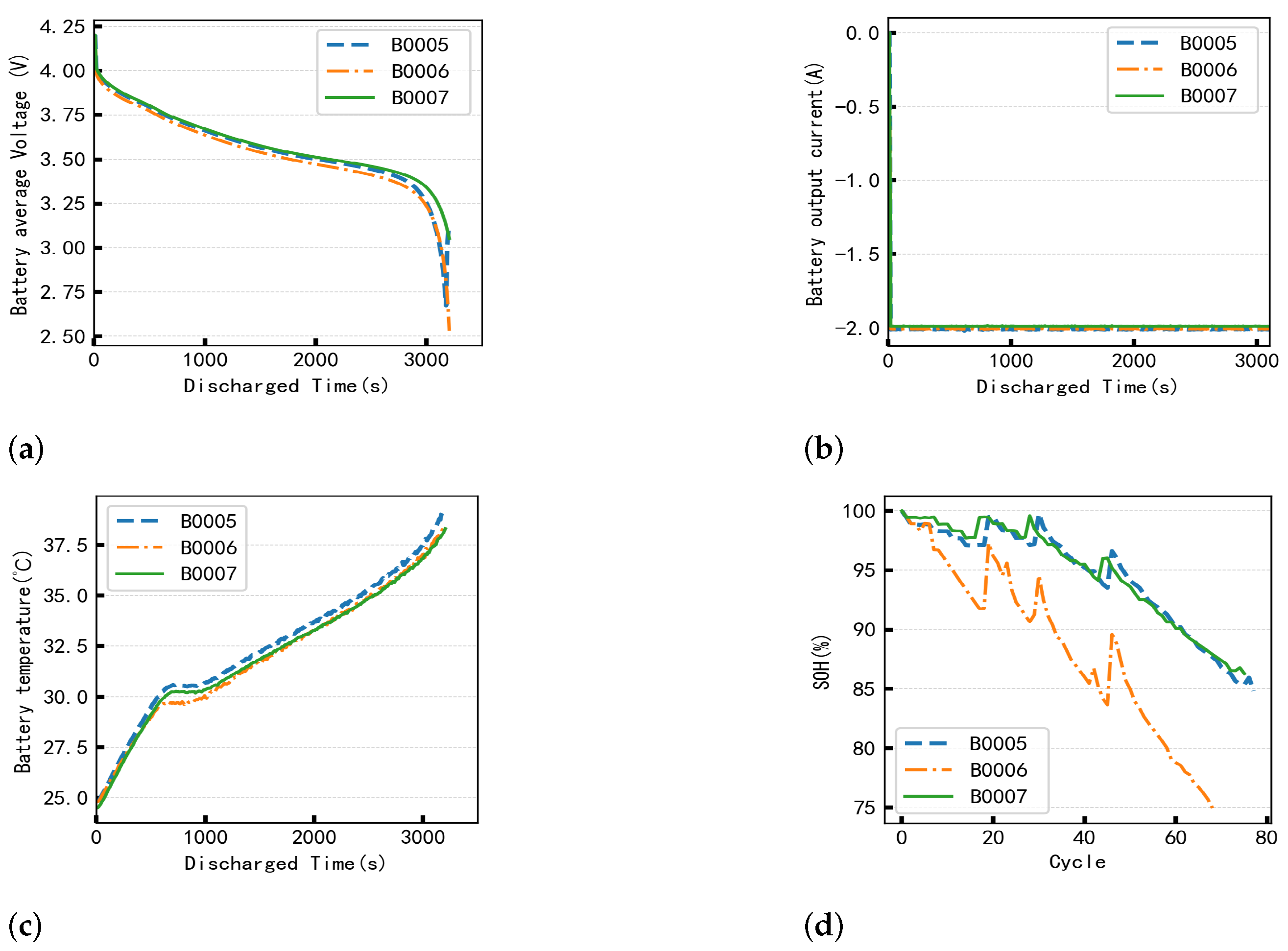
The data used in this experiment were obtained from the NASA Ames Research Center [36]. Under steady-state discharge conditions, four sets of lithium-ion battery datasets (B0005, B0006, B0007, and B0018) were collected through three different operations: charging, discharging, and impedance testing. These four battery sets (B0005, B0006, B0007, and B0018) were operated at room temperature with three different processes: charging, discharging, and impedance measurement.

For charging, the batteries were charged in a constant current (CC) mode at 1.5 A until the battery voltage reached 4.2 V, after which the charging continued in a constant voltage (CV) mode until the charging current dropped to 20 mA. For discharging, a constant current (CC) of 2 A was applied until the battery voltages for B0005, B0006, B0007, and B0018 dropped to 2.7 V, 2.5 V, 2.2 V, and 2.5 V, respectively. Impedance measurements were taken through electrochemical impedance spectroscopy (EIS), with frequency scans from 0.1 Hz to 5 kHz. Repeated charging and discharging cycles lead to accelerated aging of the batteries, while impedance measurements provide deeper insights into the internal parameter changes during battery aging. The experiment ends when the battery reaches its End of Life (EOL) criteria, defined as a 30% reduction in rated capacity (from 2.0 Ah to 1.4 Ah). This dataset is valuable for predicting the remaining capacity (for a given discharge cycle) and the Remaining Useful Life (RUL) of the batteries.

Figure 5 shows the discharge data (voltage, current, temperature, and SOH) for batteries B0005, B0006, and B0007. To verify the generalizability of the XGBoost algorithm for SOH estimation, the learning rate was set to 0.2, the minimum leaf weight was set to 1, and the tree depth was set to 3 (experimental results indicate that this model converges). Two sets of experiments were conducted: In the first set, the discharge data of B0006 and B0007 were used as the training dataset for the model, while the discharge data of B0005 were used as the test dataset to evaluate the model’s performance. In the second set, the discharge data of B0005 and B0007 were used as the training dataset, and the discharge data of B0006 were used as the test dataset to evaluate the model’s performance.

4.1. Technical Indicators

In this study, three key performance metrics were used to evaluate the model’s ability to predict the SOH of lithium-ion batteries: Mean Absolute Error (MAE), Root Mean Squared Percentage Error (RMSPE), and Maximum Error. These metrics were selected due to their complementary ability to provide a comprehensive assessment of model accuracy, robustness, and performance across various conditions. Each of these metrics offers unique insights into the prediction capabilities of the model, helping to assess different aspects of prediction performance, from average error to worst-case error.

The MAE measures the average magnitude of errors in the predictions, disregarding the direction of the error. It is calculated by averaging the absolute differences between the true values and the predicted values:

$$\begin{array}{c}\hfill \mathrm{MAE}={\displaystyle \frac{1}{n}}\sum _{i=1}^n|Y_i^{*}-Y_i|\end{array}$$

(12)

where $Y_i^{*}$ represents the true value, and $Y_i$ is the predicted value. The MAE provides a straightforward, interpretable measure of the average prediction error, making it particularly useful for evaluating the accuracy of SOH predictions. Smaller MAE values indicate better prediction accuracy on average.

The RMSPE quantifies the error as a percentage of the true value, making it sensitive to large errors due to its squared nature. It is defined as

$$\begin{array}{c}\hfill \mathrm{RMSPE}=\sqrt{{\displaystyle \frac{1}{n}}\sum _{i=1}^n{\left({\displaystyle \frac{Y_i^{*}-Y_i}{Y_i^{*}}}\right)}^2}\end{array}$$

(13)

where $Y_i^{*}$ and $Y_i$ are the true and predicted values, respectively. The RMSPE is useful in SOH prediction because it reflects both the magnitude and the relative error, offering a better understanding of model performance across different scales of data. A lower RMSPE indicates that the model is consistently accurate, even when the magnitude of the data varies.

Lastly, the Maximum Error measures the largest deviation between the true and predicted values in the dataset:

$$\begin{array}{c}\hfill \mathrm{Maximum}\mathrm{Error}=max\left(|Y_i^{*}-Y_i|\right)\end{array}$$

(14)

This metric highlights the worst-case scenario, providing insight into the largest single error that the model produces. A smaller Maximum Error indicates that the model is unlikely to produce large, problematic deviations, which is crucial in applications such as battery management systems, where even a small error can have significant implications. Together, these three metrics—MAE, RMSPE, and Maximum Error—offer a comprehensive evaluation of the model’s performance. The lower the values of these metrics, the better the model’s performance in predicting the SOH. A small MAE suggests that the model’s predictions are close to the true values on average, a low RMSPE indicates that the model performs well across varying data scales, and a small Maximum Error ensures that the model does not make large, unmanageable errors. These metrics are essential for ensuring the accuracy and reliability of SOH predictions in practical applications.

4.2. Analysis of Experimental Results

To validate the accuracy of the lithium-ion battery SOH estimation method based on the XGBoost algorithm, the predicted results are compared with those obtained from other widely used predictive models, including RF, LR, KNN, and SVM. As shown in Figure 6, this comparison offers a comprehensive evaluation of the performance of the XGBoost-based model relative to these alternative methods. By examining the predictive accuracy of multiple models, the effectiveness and robustness of the XGBoost algorithm in estimating the SOH can be thoroughly assessed, ensuring its superior performance in various scenarios.

Table 1. Error comparison of B0005 and B0006 battery datasets.

Algorithm	Battery B0005			Battery B0006
	MAE	RMSPE	Maximum Error	MAE	RMSPE	Maximum Error
XGBoost	0.001104	0.001495	0.004548	0.001025	0.001591	0.004145
RF	0.002873	0.004416	0.015743	0.004622	0.009162	0.037131
KNN	0.007067	0.009731	0.030525	0.016192	0.023421	0.061488
LR	0.019386	0.029174	0.139801	0.020203	0.031348	0.092293
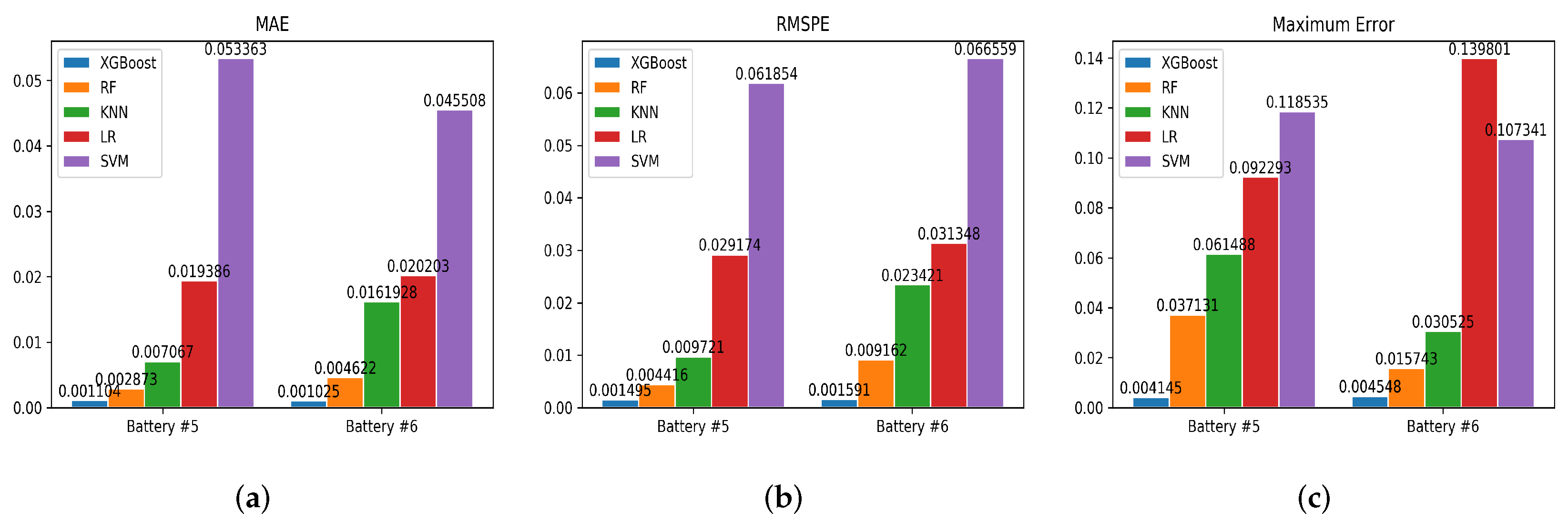
SVM	0.053363	0.061854	0.107341	0.045508	0.023421	0.061488

provides a comparative analysis of the error results for XGBoost and four other regression algorithms applied to the B0005 and B0006 datasets evaluated using three performance metrics: MAE, RMSPE, and Maximum Error. As shown in Table 1, XGBoost consistently achieved lower error values in all statistical error analysis metrics, outperforming the other algorithms. This indicates that XGBoost offers superior estimation accuracy, making it a more reliable choice compared to the other four regression algorithms. The lower error values across these key performance indicators suggest that XGBoost delivers more precise predictions of the SOH, which is crucial for battery management systems. Consequently, it can be concluded that XGBoost stands out in terms of predictive performance, offering more accurate SOH estimates, thereby enhancing the overall reliability of battery performance predictions.

As shown in Figure 7, the visual comparison of the MAE, RMSPE, and Maximum Error from Table 1 reveals that XGBoost outperformed the other four regression algorithms in both the B0005 and B0006 datasets. XGBoost achieved an error range of approximately ±0.4%, showcasing its superior estimation accuracy across all three performance metrics. This result highlights XGBoost’s ability to maintain high precision while controlling errors, offering a distinct advantage over the other algorithms in terms of both overall accuracy and error management. Consequently, XGBoost proved to be a highly reliable and effective algorithm for SOH estimation of lithium-ion batteries, demonstrating robust performance across diverse datasets.

The discharge data of lithium-ion batteries exhibit real-time characteristics, with the SOH continuously changing over time. As a result, the residuals between the predicted and actual values from the XGBoost model form a time series. To assess the stationarity of this residual time series, a unit root test (ADF test) was conducted [37], as shown in

Table 2. The XGBoost residual stationarity test results.

B0005		B0006
Metric	Value	Metric	Value
Test Statistic	−10.36947	Test Statistic	−15.56983
p-value	4.78923 × 10−30	p-value	2.58974 × 10−30
1% Critical Value	−3.51828	1% Critical Value	$-3.53692$
5% Critical Value	$-2.89987$	5% Critical Value	$-2.90788$
10% Critical Value	$-2.58722$	10% Critical Value	$-2.59149$

. Under the assumption that the residual time series has a unit root, if the test statistic is smaller than the threshold at the 1% significance level, the null hypothesis is rejected, indicating that the time series is stationary. In both the B0005 and B0006 datasets, the t-values are significantly smaller than the threshold at the 1% level, and the p-values are well below 0.05. This confirms that the residual time series of XGBoost is stationary in both datasets. By ensuring that the residuals are stationary, we can conclude that the XGBoost model’s prediction errors do not exhibit systematic trends, making the model more reliable for estimating the SOH of lithium-ion batteries.

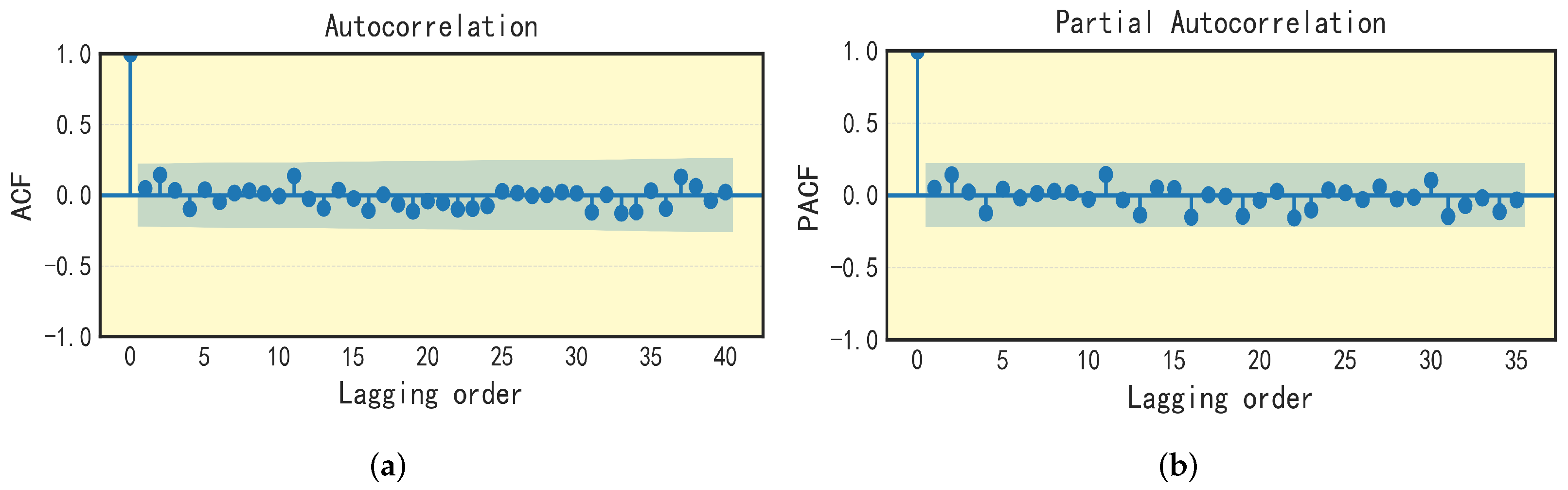
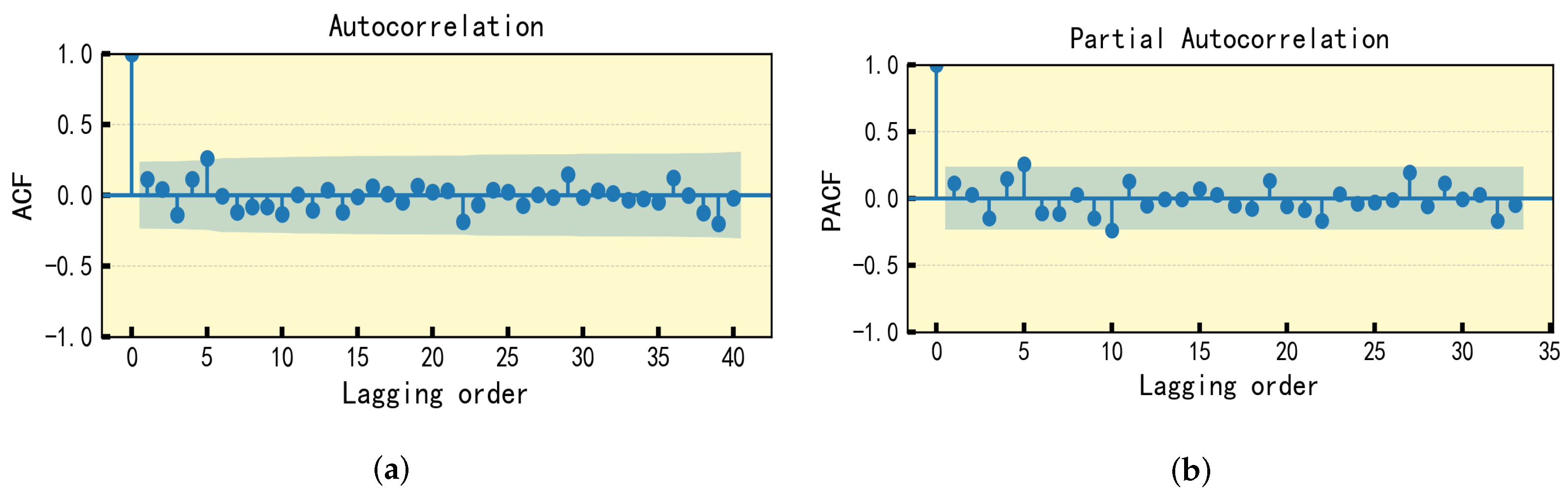
Figure 8 and Figure 9 illustrate the confidence interval, with the shaded area representing boundaries set by twice the standard deviation of the correlation coefficient. As seen in these figures, there exists a clear correlation between the residual at the current moment and historical residuals, which suggests a temporal dependency within the residual time series. This correlation indicates that by identifying patterns in past residual data, it is possible to forecast future residuals. Such findings underscore the predictive nature of residuals, offering a promising avenue to improve the accuracy of the model. The ability to predict future residuals based on historical data can significantly enhance the reliability of the SOH predictions for lithium-ion batteries, contributing to more accurate battery health management. Through analysis, it can be concluded that ARIMA (3, 0, 1) and ARIMA (2, 0, 1) are the optimal parameter solutions for the XGBoost residual time series data of the B0005 and B0006 datasets, respectively.

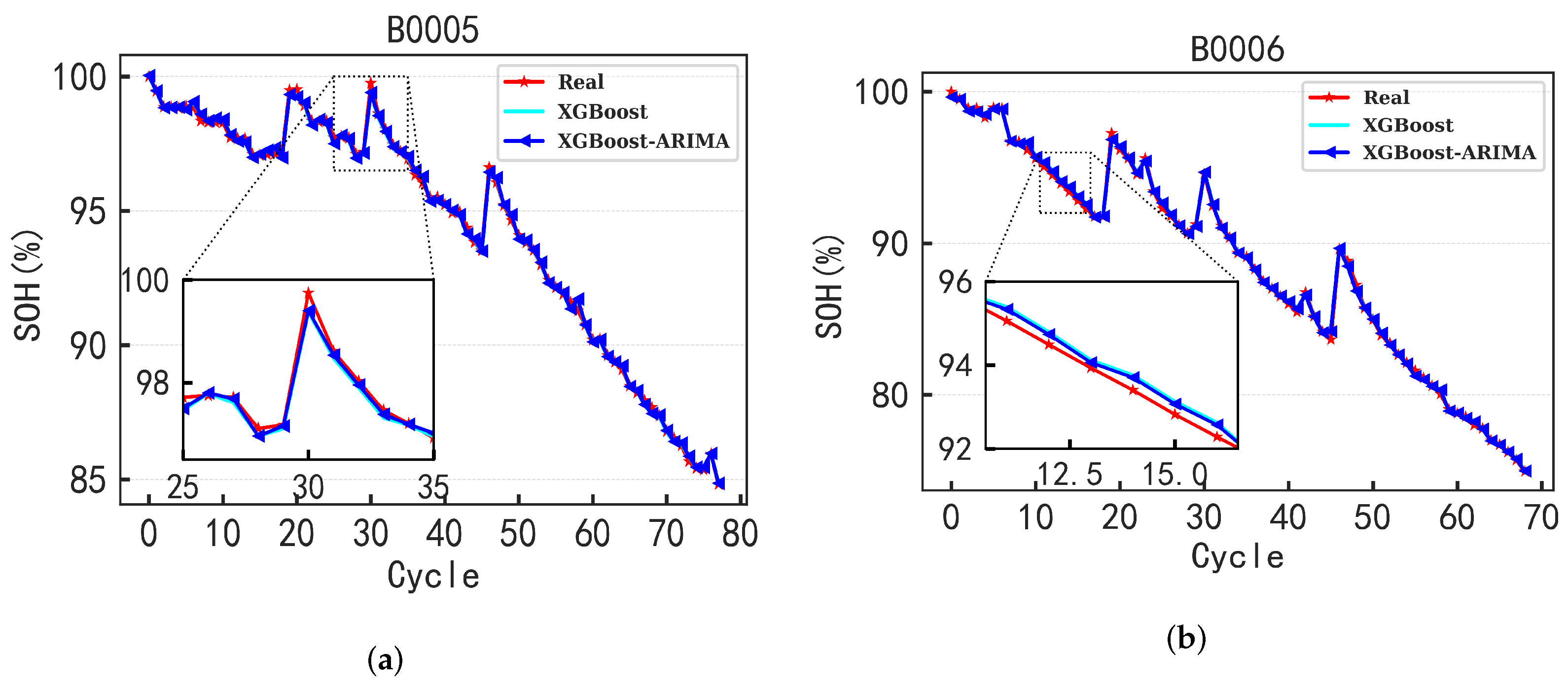
In order to further improve the reliability and accuracy of SOH prediction, this study employed a lithium-ion battery SOH estimation method based on the XGBoost–ARIMA combined model applied to two different datasets. First, the XGBoost model was used to compute the predicted values of SOH. Then, the residuals between the predicted SOH values and the actual values were treated as a new time series, which was input into the ARIMA model to correct the residuals, resulting in a more accurate SOH estimate. As shown in Figure 10, the results demonstrate that this method significantly improves the accuracy and reliability of SOH predictions. This combined approach leverages the strength of XGBoost in handling large datasets and the time series correction capability of ARIMA, offering a robust solution for predicting the health state of lithium-ion batteries.

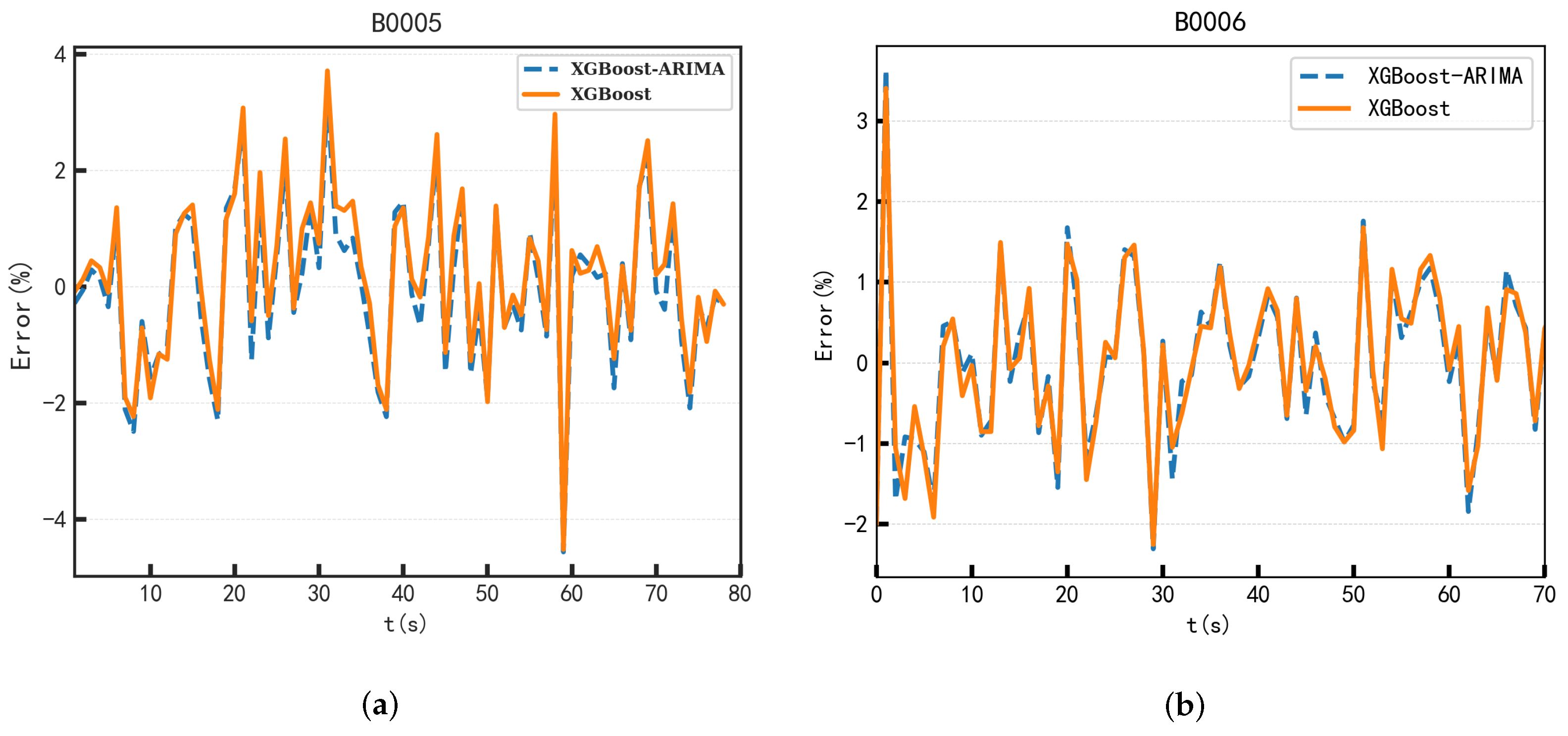
Figure 11 shows a comparison of the errors between the XGBoost–ARIMA and XGBoost predictions across different datasets. From the comparison of error results, it is evident that the errors produced by the XGBoost–ARIMA predictions fluctuate more closely around zero, with a smaller range compared to XGBoost in both datasets. This suggests that the SOH predictions made by the XGBoost–ARIMA model are closer to the actual values, and the XGBoost–ARIMA model demonstrates better stability in SOH estimation over long time series compared to XGBoost. The improved stability of the XGBoost–ARIMA model highlights its suitability for long-term SOH predictions, where stability and accurate error reduction are crucial for ensuring reliable battery health management over time.

5. Conclusions

This paper presents an intelligent estimation method for the SOH of lithium-ion batteries based on the XGBoost–ARIMA combined model. By analyzing the key features in the battery discharge process, it was found that voltage difference, temperature difference, and average voltage can effectively reflect the aging characteristics of the battery. Therefore, these three features were selected as input variables for SOH estimation. Then, the XGBoost model was used to predict the SOH, learning the underlying patterns of battery health from the input features. To further improve the prediction accuracy, the ARIMA model was introduced to correct the residuals of the XGBoost predictions, optimizing the final SOH estimate. To validate the effectiveness of this method, the XGBoost–ARIMA combined model was compared with five other mainstream regression algorithms, including RF, KNN, LR, and SVM. The experimental results show that the XGBoost–ARIMA combined model outperformed the other five regression algorithms in terms of estimation accuracy on both the B0005 and B0006 datasets. Specifically, the XGBoost–ARIMA model is able to control the SOH prediction error within a smaller range and exhibits higher stability and stronger generalization ability in long-term sequence predictions. In conclusion, the XGBoost–ARIMA combined model provides a highly efficient and reliable solution for lithium-ion battery health management.

Although our approach has shown promising results in a controlled experimental environment, there are some limitations to be addressed. Firstly, the model currently relies on specific datasets (such as the NASA dataset), which may limit its generalizability to other types of batteries or different application scenarios. Therefore, future research could validate the method on more diverse battery datasets to assess its applicability across various battery types and operating conditions. Secondly, although the XGBoost–ARIMA model performs well in terms of accuracy, its adaptability to complex battery characteristics (e.g., internal resistance, cycle count, etc.) and different aging conditions may present challenges. As such, we plan to further optimize feature selection by incorporating additional battery features, which could improve the model’s robustness and generalization ability across diverse use cases. Furthermore, the accuracy of the model may be affected by data quality issues in practical applications. Future work could address this by integrating data enhancement and online learning methods to improve data quality and enhance model stability.

Although this paper demonstrates good accuracy in a controlled experimental setting, applying this method in real-world battery management systems presents a number of challenges. First, battery management systems typically require real-time monitoring and quick decision making. Hence, improving the model’s computational efficiency and real-time responsiveness, while ensuring high accuracy, is a critical challenge. Additionally, real-world applications often face data quality issues, such as sensor failures or missing data, which can impact the prediction accuracy. Future work could explore techniques like data imputation and augmentation to improve data quality. Furthermore, efficiently deploying the model in embedded devices or industrial-scale battery management systems remains a technical challenge, including limitations in hardware resources and energy consumption. As a result, we plan to focus on improving the computational efficiency and deployability of the model in future research, combining deep learning techniques with traditional statistical methods to enhance prediction accuracy and address real-time concerns.

References

1. Xu, Q.; Zhang, L.; Liang, C.; Li, Y. Short-term Load Forecasting for Power System with High Proportion New Energy Based on Joint Sequential Scenario and Improved TCN. Guangdong Electr. Power 2024, 37, 1–7. [Google Scholar]
2. Wang, S.; Wang, L.; Wang, G.; Zhong, Q.; Zeng, D. SOC Balancing and Power Distribution Strategies Based on Second-order Consensus Algorithm. Guangdong Electr. Power 2024, 37, 1–9. [Google Scholar]
3. Roman, D.; Saxena, S.; Robu, V.; Pecht, M.; Flynn, D. Machine learning pipeline for battery state-of-health estimation. Nat. Mach. Intell. 2021, 3, 447–456. [Google Scholar] [CrossRef]
4. Jin, J.; Yu, R.; Liu, G.; Xu, L.; Ma, Y.; Wang, H.; Hu, C. Research Progress on State-of-health Estimating Method for Lithium-ion Batteries. J. Electr. Eng. 2024, 19, 33–48. [Google Scholar]
5. Zhao, L.; W, X.; Liu, R.; He, P. Status of safety evaluation standards for Li-ion battery for energy storage. Battery Bimon. 2024, 54, 239–243. [Google Scholar]
6. Deng, Z.; Hu, X.; Li, P.; Lin, X.; Bian, X. Data-driven battery state of health estimation based on random partial charging data. IEEE Trans. Power Electron. 2021, 37, 5021–5031. [Google Scholar] [CrossRef]
7. Hu, H.; Pang, Z. State of Health Estimation of Lithium-ion Batteries for Vehicles. Automob. Appl. Technol. 2023, 48, 1–4. [Google Scholar]
8. Zhai, S.; Li, W.; Zhou, C.; Wang, C.; Hou, S. State-of-Charge Estimation of Energy Storage Batteries Based on Modified Probabilistic Neural Networks. Smart Power 2024, 52, 94–100. [Google Scholar]
9. Guo, R.; Shen, W. A review of equivalent circuit model based online state of power estimation for lithium-ion batteries in electric vehicles. Vehicles 2021, 4, 1–29. [Google Scholar] [CrossRef]
10. Wu, H.; Shao, S.; Dai, J.; Zhang, Z.; Peng, W. Study on the correlation of two kinds of internal resistance measurement approaches for lithium-ion battery. J. Hefei Univ. Technol. 2023, 46, 1003–1008. [Google Scholar]
11. Shi, Y.; Wang, L.; Gong, M. Research on prediction of remaining useful life of lithium-ion batteries based on convolutional attention mechanism. J. Southwest Minzu Univ. 2024, 50, 336–346. [Google Scholar]
12. Guo, Y.; Yu, P.; Zhu, C.; Zhang, K.; Wang, L.; Wang, K. A state-of-health estimation method considering capacity recovery of lithium batteries. Int. J. Energy Res. 2022, 46, 23730–23745. [Google Scholar] [CrossRef]
13. Gou, B.; Xu, Y.; Feng, X. State-of-health estimation and remaining-useful-life prediction for lithium-ion battery using a hybrid data-driven method. IEEE Trans. Veh. Technol. 2020, 69, 10854–10867. [Google Scholar] [CrossRef]
14. Zhou, J.; Yan, Z.; Li, M. Life prediction of lithium-ion battery based on evolutionary algorithm and data-driven approach. Chin. J. Power Sources 2024, 48, 679–684. [Google Scholar]
15. Hong, S.; Yue, T.; Liu, H. Vehicle energy system active defense: A health assessment of lithium-ion batteries. Int. J. Intell. Syst. 2022, 37, 10081–10099. [Google Scholar] [CrossRef]
16. Yao, F.; Zhang, N.; Huang, K. Review of State Estimation and Life Prediction for Lithium-ion Batteries. J. Power Supply 2020, 18, 175–183. [Google Scholar]
17. Bian, X.; Wei, Z.; Li, W.; Pou, J.; Sauer, D.U.; Liu, L. State-of-health estimation of lithium-ion batteries by fusing an open circuit voltage model and incremental capacity analysis. IEEE Trans. Power Electron. 2021, 37, 2226–2236. [Google Scholar] [CrossRef]
18. She, C.; Li, Y.; Zou, C.; Wik, T.; Wang, Z.; Sun, F. Offline and Online Blended Machine Learning for Lithium-Ion Battery Health State Estimation. IEEE Trans. Transp. Electrif. 2021, 8, 1604–1618. [Google Scholar] [CrossRef]
19. Gao, Y.; Liu, K.; Zhu, C.; Zhang, X.; Zhang, D. Co-estimation of state-of-charge and state-of-health for lithium-ion batteries using an enhanced electrochemical model. IEEE Trans. Ind. Electron. 2021, 69, 2684–2696. [Google Scholar] [CrossRef]
20. Liu, Y.; Wang, L.; Li, D.; Wang, K. State-of-health estimation of lithium-ion batteries based on electrochemical impedance spectroscopy: A review. Prot. Control. Mod. Power Syst. 2023, 8, 1–17. [Google Scholar] [CrossRef]
21. Zhang, Q.; Huang, C.G.; Li, H.; Feng, G.; Peng, W. Electrochemical impedance spectroscopy based state-of-health estimation for lithium-ion battery considering temperature and state-of-charge effect. IEEE Trans. Transp. Electrif. 2022, 8, 4633–4645. [Google Scholar] [CrossRef]
22. Liu, D.; Pang, J.; Zhou, J.; Peng, Y.; Pecht, M. Prognostics for state of health estimation of lithium-ion batteries based on combination Gaussian process functional regression. Microelectron. Reliab. 2013, 53, 832–839. [Google Scholar] [CrossRef]
23. Li, N.; He, F.; Ma, W.; Wang, R.; Jiang, L.; Zhang, X. An indirect state-of-health estimation method based on improved genetic and back propagation for online lithium-ion battery used in electric vehicles. IEEE Trans. Veh. Technol. 2022, 71, 12682–12690. [Google Scholar] [CrossRef]
24. Ren, P.; Wang, S.; Chen, X.; Huang, J. Fusion estimation strategy based on dual adaptive Kalman filtering algorithm for the state of charge and state of health of hybrid electric vehicle Li-ion batteries. Int. J. Energy Res. 2022, 46, 7374–7388. [Google Scholar] [CrossRef]
25. Li, J.; Ye, M.; Gao, K.; Xu, X.; Wei, M.; Jiao, S. Joint estimation of state of charge and state of health for lithium-ion battery based on dual adaptive extended Kalman filter. Int. J. Energy Res. 2021, 45, 13307–13322. [Google Scholar] [CrossRef]
26. Chaoui, H.; Ibe-Ekeocha, C.C. State of charge and state of health estimation for lithium batteries using recurrent neural networks. IEEE Trans. Veh. Technol. 2017, 66, 8773–8783. [Google Scholar] [CrossRef]
27. Wei, M.; Wang, Q.; Ye, M.; Li, J.; Xu, X. An indirect remaining useful life prediction of lithium-ion batteries based on a NARX dynamic neural network. Chin. J. Eng. 2022, 44, 380–388. [Google Scholar]
28. Sun, S.; Sun, J.; Wang, Z.; Zhou, Z. Prediction of battery SOH by CNN-BiLSTM network fused with attention mechanism. Energies 2022, 15, 4428. [Google Scholar] [CrossRef]
29. Jia, J.; Wang, K.; Pang, X.; Shi, Y.; Wen, J.; Zeng, J. Multi-Scale prediction of RUL and SOH for Lithium-Ion batteries based on WNN-UPF combined model. Chin. J. Electron. 2021, 30, 26–35. [Google Scholar]
30. Asselman, A.; Khaldi, M.; Aammou, S. Enhancing the prediction of student performance based on the machine learning XGBoost algorithm. Interact. Learn. Environ. 2023, 31, 3360–3379. [Google Scholar] [CrossRef]
31. Xing, Z.; Chu, J.; Wang, K.; Wu, S. Prediction of rockhead using a hybrid N-XGBoost machine learning framework. J. Rock Mech. Geotech. Eng. 2021, 13, 1231–1245. [Google Scholar]
32. Wang, Y.; Zhou, K.; Shen, S. A state transition prediction model based on XGBoost algorithm. J. Zhejiang Univ. Technol. 2024, 52, 275–279. [Google Scholar]
33. Sahai, A.K.; Rath, N.; Sood, V.; Singh, M.P. ARIMA modelling & forecasting of COVID-19 in top five affected countries. Diabetes Metab. Syndr. Clin. Res. Rev. 2020, 14, 1419–1427. [Google Scholar]
34. Kufel, T. ARIMA-based forecasting of the dynamics of confirmed COVID-19 cases for selected European countries. Equilib. Q. J. Econ. Econ. Policy 2020, 15, 181–204. [Google Scholar] [CrossRef]
35. Lai, Y.; Dzombak, D.A. Use of the autoregressive integrated moving average (ARIMA) model to forecast near-term regional temperature and precipitation. Weather. Forecast. 2020, 35, 959–976. [Google Scholar] [CrossRef]
36. Saha, B.; Goebel, K. NASA Ames Prognostics Data Repository: Battery Data Set [DS/OL]; NASA Ames Research Center: Mountain View, CA, USA, 2007. Available online: http://ti.arc.nasa.gov/project/pRognostic-data-repository (accessed on 19 May 2025).
37. Chen, G.; Guo, P.; Pi, H.; Sun, C.; Li, C. Regressive Moving Average Model Time Series Analysis of Pier Displacement Stability Based on Unit Root Test and Auto-Regressive Moving Average Model. J. Wuhan Inst. Technol. 2023, 45, 586–590. [Google Scholar]
Figure 1. The flow chart of extreme gradient boosting.
Batteries 11 00207 g001
Figure 2. Characteristic change curves: (a) the voltage variation curves of lithium-ion batteries under different SOH conditions are displayed; (b) the temperature variation curves of lithium-ion batteries under different SOH conditions are displayed; (c) the SOC variation curves of lithium-ion batteries under different SOH conditions are displayed; (d) the current variation curves of lithium-ion batteries under different SOH conditions are displayed.
Batteries 11 00207 g002
Figure 3. System framework diagram.
Batteries 11 00207 g003
Figure 4. Block diagram based on the XGBoost–ARIMA model.
Batteries 11 00207 g004
Figure 5. Discharge data, (ad) respectively represent the voltage, current, temperature, and SOH discharge data for B0005, B0006, and B0007.
Batteries 11 00207 g005
Figure 6. Comparison of prediction results: (a) comparison of SOH prediction results for dataset B0005, (b) comparison of SOH prediction results for dataset B0006.
Batteries 11 00207 g006
Figure 7. Error visualization comparison: (ac) respectively represent the MSE, RMSE, and Maximum Error of datasets B0005 and B0006 under different algorithms.
Batteries 11 00207 g007
Figure 8. Autocorrelation and partial autocorrelation coefficients of XGBoost residuals for dataset B0005: (a) autocorrelation coefficients of XGBoost residuals based on dataset B0005, (b) partial autocorrelation coefficients of XGBoost residuals based on dataset B0005.
Batteries 11 00207 g008
Figure 9. Autocorrelation and partial autocorrelation coefficients of XGBoost residuals for dataset B0006: (a) autocorrelation coefficients of XGBoost residuals based on dataset B0006, (b) partial autocorrelation coefficients of XGBoost residuals based on dataset B0006.
Batteries 11 00207 g009
Figure 10. Comparison of prediction results based on XGBoost and XGBoost–ARIMA models: (a) comparison of SOH prediction results between XGBoost and XGBoost–ARIMA for dataset B0005, (b) comparison of SOH prediction results between XGBoost and XGBoost–ARIMA for dataset B0006.
Batteries 11 00207 g010
Figure 11. Comparison of prediction errors based on XGBoost and XGBoost–ARIMA models: (a) comparison of SOH prediction errors between XGBoost and XGBoost–ARIMA for dataset B0005, (b) comparison of SOH prediction errors between XGBoost and XGBoost–ARIMA for dataset B0006.
Batteries 11 00207 g011