Prediction of the Remaining Useful Life of Lithium–Ion Batteries Based on Mode Decomposition and ED-LSTM

Abstract

The prediction of remaining useful life (RUL) of lithium–ion batteries is key to the reliability assessment of batteries and affects safe application of batteries. This article introduces a CEEMDAN-RF-MHA-ED-LSTM method. Using CEEMDAN, the battery capacity data were decomposed to obtain intrinsic mode functions (IMFs), and the weight of each IMF was obtained via the random forest (RF) algorithm. The LSTM neural network was used, the encoder–decoder (ED) structure was introduced, the multi-head attention (MHA) mechanism was used to construct a network model, and the particle swarm optimization (PSO) algorithm was used to optimize the model parameters. Each IMF was input into the model, and the obtained forecast results were weighted and reconstructed to obtain the final forecast data. This method was validated on the battery dataset released by NASA. Compared with that of the single LSTM model, the mean absolute error of the proposed method decreases by 74%, 62%, 71%, and 55% on the No. 05, 06, 07, and 18th battery datasets, respectively. The root mean square error decreased by 72%, 59%, 70%, and 54%, and the mean absolute percent error decreased by 75%, 65%, 71%, and 58%, respectively. This method can accurately predict battery RUL.

1. Introduction

Relying on the advantages of high energy conversion efficiency, low pollution and convenient maintenance, electric vehicles have become the core of the automotive industry [1,2]. Compared with traditional batteries such as lead–acid batteries, lithium–ion batteries are being used in batches in electric vehicles because of their advantages, such as high energy density, low self-discharge rate, long cycle life, energy savings and environmental protection. However, as the number of batteries used and the number of charge–discharge cycles increase, the capacity and reliability of the battery decreases, and safety decreases significantly [3,4,5,6]. Therefore, it is particularly important to predict the RUL of lithium–ion batteries.

For RUL prediction methods, at present, model-based and data-driven methods are mainly used [7,8,9,10,11]. In the model-based prediction method, on the basis of familiarity with the internal structure of batteries and related physical and chemical theories, a physical model or electrochemical model is created to simulate the performance degradation process of Li-ion batteries. Alipour [12] et al. established an electrochemical–thermal aging model for commercial batteries via a bidirectional coupling method and performed uncertainty quantitative analysis on the coupled electrochemical–thermal aging model to improve the reliability of the battery model. Moreover, the effects of parametric model uncertainties on battery voltage, temperature, and aging were investigated. Xia Quan [13] et al. combined the coupled electrochemical model, equivalent circuit model, heat transfer model and fluid dynamics model to evaluate and predict the capacity and reliability of batteries. Battery changes are complex in the actual use process, model-based methods are susceptible to the influence of variable current and temperature, and there are uncertainties in the accuracy of the model. In addition, under the influence of different external conditions, it is not easy to obtain an accurate model. The data-driven prediction method analyses the degradation mode of the training data and updates the network parameters to establish the degradation mapping relationship between the training data and the test data, which is more flexible and convenient. The most widely used methods are support vector machine (SVM) and relevance vector machine (RVM), as well as Gaussian process regression (GPR). Wang Xiuli [14] et al. used the expectation maximization algorithm to update time-varying parameters and combined it with the RVM algorithm to establish a multistep forecasting model. However, owing to the high sparsity of the RVM, RVM-based prediction methods are often not stable enough. Li Xiaoyu [15] et al. extracted four important features from different angles, such as the intercept, slope, and peak value, through analysis of partial incremental capacity and applied the GPR of nonlinear regression to predict the battery health status. However, the hyperparameter tuning process of GPR is complicated and difficult to model.

In addition to the above data-driven methods, artificial neural networks (ANNs) have better learning ability in complex system modeling. M Catelani [16] et al. introduced state detection and a recurrent neural network (RNN) for battery capacity prediction and used the capacity data provided by state detection for training the RNN model. Although RNNs can predict future trends on the basis of historical information, they have the problem of gradient disappearance or gradient explosion. Wu Minghu [17] et al. proposed a prediction model for the RUL of lithium batteries that combined ensemble empirical mode decomposition (EEMD) and a gated cyclic unit network (GRU). However, the GRU still performs poorly in processing long-term series information. S Zheng [18] et al. used long short-term memory (LSTM) to predict battery life. LSTM can effectively capture long term dependency of sequential data and provide more accurate prediction results. However, the original data contain noise. If the data are not denoised, the effectiveness of the prediction will be affected. Wang Pengkai [19] et al. utilizing deep residual networks to extract the hidden feature information of the original data and then used a bidirectional long short-term memory (BiLSTM) network to make predictions, which have added attention mechanisms to distribute weights for the prediction results to optimize the RUL predictive performance. Song Wenbin [20] et al. proposed a transformer-based lithium–ion RUL prediction method, which added a denoising autoencoder to denoise the original data and designed a time encoding layer to further optimize predictive performance. Although the above methods can denoise to a certain extent, they are still affected by the battery capacity regeneration phenomenon, which reduces the accuracy of RUL prediction. The modal decomposition method can alleviate the influence of the difficult-to-capture battery capacity regeneration phenomenon. Li Yang et al. [21] used the EEMD method to decompose battery capacity data; the selected IMF reflects the degradation of lithium batteries, and a Gaussian process regression model is constructed on the basis of the IMF. Although EEMD can separate the noise components in the data, it has the problem of mode aliasing. Xiao Haoyi [22] et al. used the complete ensemble empirical mode decomposition with adaptive noise (CEEMDAN) method to decompose data combined with the RF algorithm for each intrinsic mode. The IMF distributes weights, and the prediction results of different IMFs are reconstructed with weights to achieve accurate prediction of the RUL of lithium–ion batteries.

In this paper, battery capacity is used as an indicator of health status, and a lithium battery RUL prediction method called the CEEMDAN-RF-MHA-ED-LSTM is proposed. This method first uses CEEMDAN to convert the raw data into multiple IMFs to alleviate the impact of the battery capacity regeneration phenomenon on RUL prediction; then, the RF is used to obtain the weight of each IMF. The features of decomposed data are extracted through an LSTM neural network with an ED structure. To more effectively capture the global features and dependencies of the sequence, the MHA mechanism was introduced into the prediction model. Using the PSO algorithm, the parameters of the constructed model were optimized by comparing the error indicators of the IMF with the highest weight under different model parameter combinations. The prediction result obtained by each IMF is calculated by the weight obtained by the RF. Weighted reconstruction is used to obtain the final predicted value. On the basis of the analysis of the above methods, the combined method has a good effect on the RUL prediction of lithium batteries in theory. In this paper, NASA’s public dataset for lithium–ion batteries is used to test the predictive performance of this method.

2. Results and Discussion

2.1. Performance of Various Neural Network Models

To verify the reliability of the CEEMDAN-RF-MHA-ED-LSTM method, this paper first compared a single neural network LSTM, GRU, with the ED-LSTM and MHA-ED-LSTM neural networks on the NASA battery dataset. ED-LSTM is a decoder-encoder structure constructed through LSTM neural network, while MHA-ED-LSTM connects attention mechanism on the basis of Encoder-Decoder structure, focusing on key information to better capture the dependencies between sequences. Figure 1 shows a comparison of the fitting effect of various models on the B0005 dataset.

Table 1. Prediction evaluation metrics of various neural network models.

Battery No.	Neural Network Model	MAE	RMSE	MAPE	RE
B 0005	GRU	0.075644	0.087753	0.051511	0.350515
	LSTM	0.067140	0.076802	0.045402	0.288659
	ED-LSTM	0.044260	0.052524	0.028345	0.144329
	MHA-ED-LSTM	0.033218	0.040826	0.021099	0.092783
B 0006	GRU	0.071366	0.092261	0.050219	0.130434
	LSTM	0.060545	0.075717	0.042193	0.123188
	ED-LSTM	0.048999	0.060832	0.032040	0.152173
	MHA-ED-LSTM	0.037996	0.047440	0.025036	0.084112
B 0007	GRU	0.069255	0.082715	0.043676	0.120967
	LSTM	0.053274	0.065517	0.033295	0.080645
	ED-LSTM	0.045779	0.054149	0.028446	0.233870
	MHA-ED-LSTM	0.031084	0.038186	0.018959	0.153225
B 0018	GRU	0.069713	0.082386	0.047055	0.333333
	LSTM	0.054881	0.068166	0.037720	0.052631
	ED-LSTM	0.040723	0.050489	0.027166	0.157894
	MHA-ED-LSTM	0.030054	0.035797	0.020037	0.017543

shows the evaluation metrics of various models on four datasets. The above results indicate that, for a single neural network, the error index of the LSTM is reduced by 10%~20% on average compared with that of the GRU, and the prediction accuracy is greater; however, the fitting effect needs to be improved. Therefore, in this paper, LSTM is used to construct the ED-LSTM neural network model.

All the error indicators of the ED-LSTM decreased significantly compared with those of the single LSTM, with the error indicators decreasing by 20% to 30% on average, and the predicted value curve also showed a better fitting trend. However, considering that the single ED structure still has deficiencies such as the loss of key information and the difficulty in information integration, the MHA mechanism is introduced in this structure to form the MHA-ED-LSTM neural network model, which reduces the risk of information loss when processing long sequences. The results in the table show that, compared with those of the ED-LSTM, the error indicators of the MHA-ED-LSTM model have further decreased; the error indicators have decreased by approximately 25% on average, but there is still a certain gap compared with the true value. Because there is a large amount of noise in the original data, this affects the accuracy of prediction.

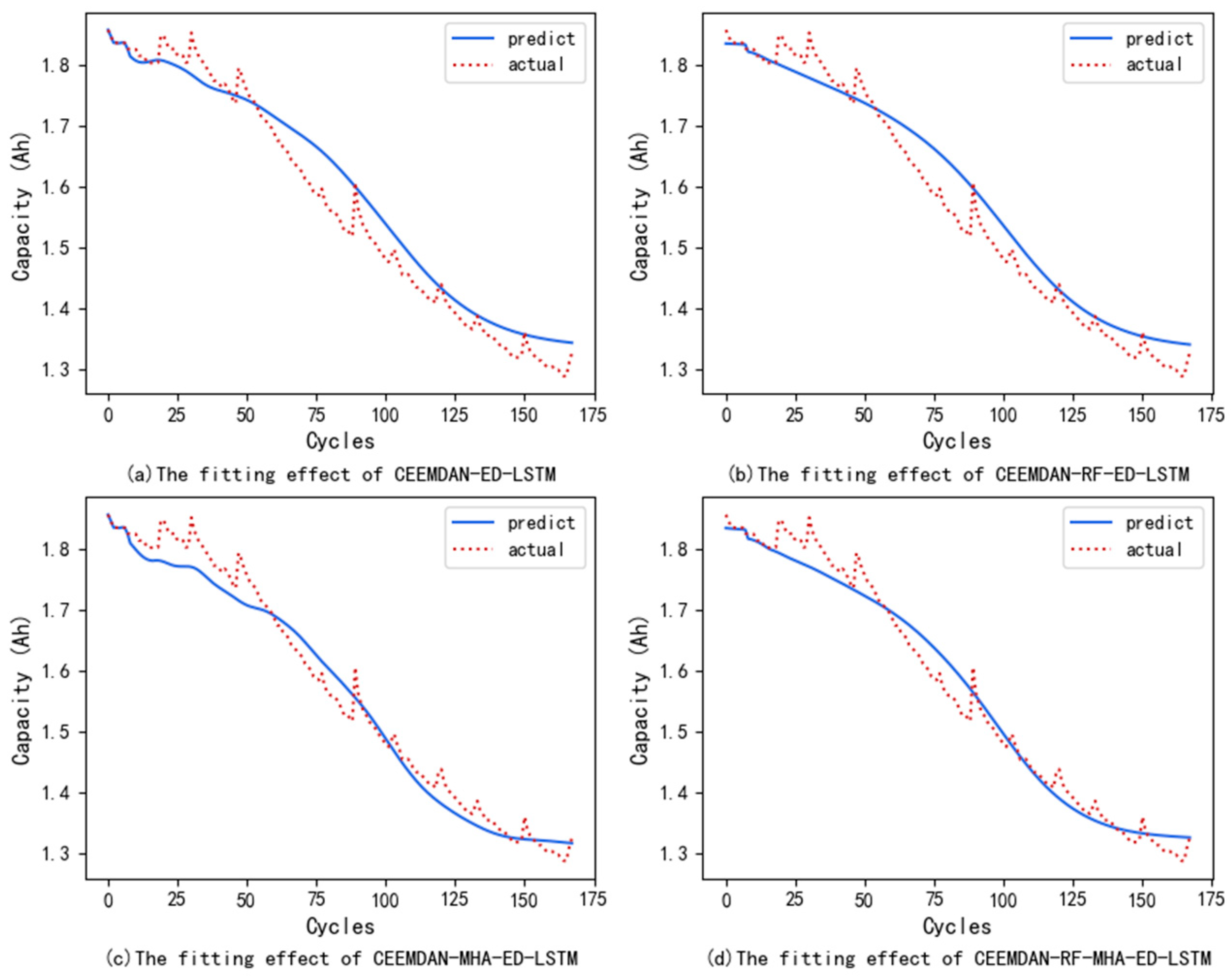
2.2. Performance of Various Combination Methods

Then, from the perspective of method combination, the NASA battery dataset was used for model comparison. The CEEMDAN + neural network model decomposes the original data using CEEMDAN, and then inputs the decomposed data into the neural network model for training and prediction. The CEEMDAN + RF + neural network model refers to using RF to assign weights to the decomposed data after data decomposition. In the prediction stage, the prediction results of each component are reconstructed based on these weights.

Table 2. Prediction evaluation metrics of various combination methods.

Battery No.	Neural Network Model	MAE	RMSE	MAPE	RE
B 0005	CEEMDAN-ED-LSTM	0.029423	0.035868	0.019226	0.072164
	CEEMDAN-MHA-ED-LSTM	0.024596	0.029906	0.015384	0.010309
	CEEMDAN-RF-ED-LSTM	0.028877	0.035308	0.018778	0.061855
	CEEMDAN-RF-MHA-ED-LSTM	0.022165	0.028269	0.014006	0.020618
B 0006	CEEMDAN-ED-LSTM	0.034582	0.043089	0.022931	0.074766
	CEEMDAN-MHA-ED-LSTM	0.030251	0.040926	0.019499	0.009345
	CEEMDAN-RF-ED-LSTM	0.033546	0.039977	0.022228	0.065420
	CEEMDAN-RF-MHA-ED-LSTM	0.029409	0.038404	0.019269	0.009345
B 0007	CEEMDAN-ED-LSTM	0.035636	0.042953	0.021779	0.169354
	CEEMDAN-MHA-ED-LSTM	0.026179	0.031930	0.015737	0.104838
	CEEMDAN-RF-ED-LSTM	0.027204	0.034353	0.016675	0.153225
	CEEMDAN-RF-MHA-ED-LSTM	0.019272	0.023959	0.011683	0.056452
B 0018	CEEMDAN-ED-LSTM	0.028369	0.038278	0.018486	0.157894
	CEEMDAN-MHA-ED-LSTM	0.024173	0.031518	0.015657	0.105263
	CEEMDAN-RF-ED-LSTM	0.027283	0.032260	0.017828	0.035087
	CEEMDAN-RF-MHA-ED-LSTM	0.025992	0.033317	0.016333	0.052631

lists the calculation results of each evaluation index for neural network prediction after the original data are decomposed via CEEMDAN. Figure 2 shows the fitting effects of various combination methods on B0005.

The models of the combination method in Table 2 are based on the neural network and use CEEMDAN to denoise the battery capacity data. The results in the table show that, after the CEEMDAN decomposition is used, the prediction is superior to that of the other methods. For example, the error index of CEEMDAN-ED-LSTM was reduced by 20%~30% on average compared with that of ED-LSTM. In addition, after the MHA-ED-LSTM neural network model uses CEEMDAN for data decomposition, the prediction curve, which was originally poorly fitted, now closely matches the true value curve. After the prediction results were adjusted via the weights of the IMF, a comparison of the four sets of error indicators, namely, the MAE, RMSE, MAPE, and RE, revealed that most of them were more accurate than the CEEMDAN + neural network method alone.

2.3. Performance of Optimized Neural Network Model

In addition, the model parameters are optimized via PSO for the best performing CEEMDAN-RF-MHA-ED-LSTM model.

Table 3. Prediction evaluation index results for the four battery datasets.

Battery No.	Neural Network Model	MAE	RMSE	MAPE	RE
B 0005	CEEMDAN-RF-MHA-ED-LSTM	0.017649	0.021791	0.011245	0.007729
B 0006	CEEMDAN-RF-MHA-ED-LSTM	0.023003	0.031283	0.014827	0.028037
B 0007	CEEMDAN-RF-MHA-ED-LSTM	0.015660	0.019705	0.009528	0.056451
B 0018	CEEMDAN-RF-MHA-ED-LSTM	0.024758	0.031219	0.015687	0.126315

lists the evaluation indicators of the final prediction model after optimization of the model parameters on the four battery datasets.

In general, the prediction accuracy of the CEEMDAN-RF-MHA-ED-LSTM method is relatively high; the prediction error indicators MAE and RMSE of the four groups of batteries are controlled at approximately 2% and 3%, respectively. To show the predictive ability of each model more intuitively, Figure 3 shows the evaluation metrics for each model on battery B0005.

A comparison of the evaluation indicators reveals that after the ED-LSTM neural network was constructed by using LSTM, the MHA was introduced, the original data were processed by CEEMDAN, and the error indicator decreased significantly.

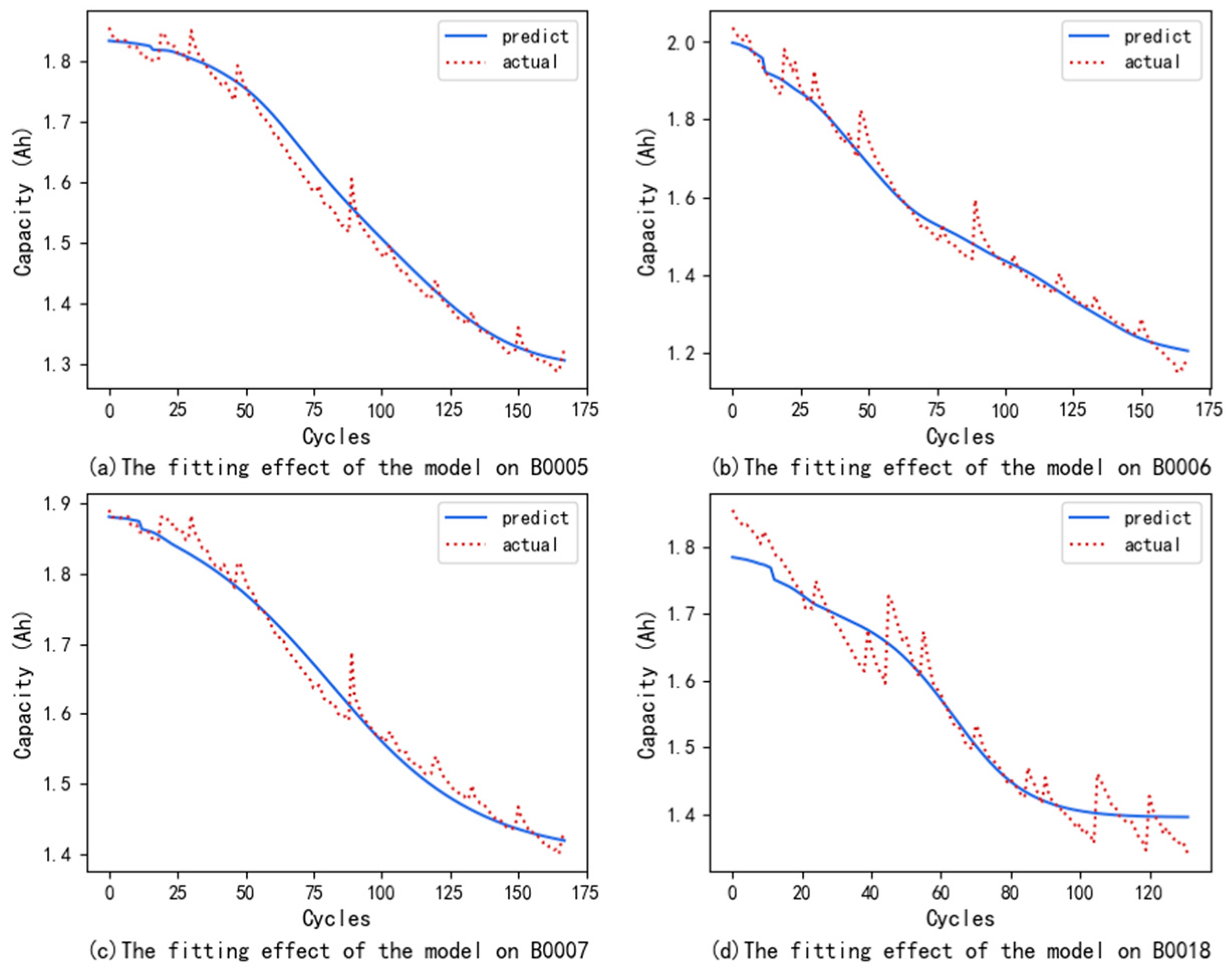
Figure 4 shows the fitting effect of the optimized neural network model on four datasets. After the model parameters of the CEEMDAN-RF-MHA-ED-LSTM method were optimized through PSO, the fitting results of the predicted value curve and the actual value curve improved. Compared with those of the single LSTM model, the mean absolute errors of the proposed method are 74%, 62%, 71% and 55% lower, the root mean square errors are 72%, 59%, 70% and 54% lower, and the mean absolute percentage errors are 75%, 65%, 71%, and 58% lower, respectively, indicating high accuracy in battery RUL prediction.

2.4. Validation of Model Generalization

Considering the complexity of the model structure, which may lead to overfitting, we divided the dataset into a 60% training set and a 40% testing set to demonstrate the model’s generalization ability. We trained the model using a training set and evaluated its final performance using an independent test set. The independent test set can provide the model’s true performance on unknown data, preventing overfitting during the training process. The prediction performance on the test set is shown in Figure 5.

In order to more accurately demonstrate the prediction performance, we used three evaluation metrics for error calculation, and the evaluation results are shown in

Table 4. Prediction evaluation index results for the four test datasets.

Battery No.	Neural Network Model	MAE	RMSE	MAPE
B 0005	CEEMDAN-RF-MHA-ED-LSTM	0.010462	0.012384	0.007701
B 0006	CEEMDAN-RF-MHA-ED-LSTM	0.015503	0.019175	0.011881
B 0007	CEEMDAN-RF-MHA-ED-LSTM	0.008630	0.010772	0.005775
B 0018	CEEMDAN-RF-MHA-ED-LSTM	0.018723	0.023641	0.013347

.

The performance of the model on the test set is comparable to that on the training set, indicating good generalization and no overfitting.

2.5. The Computational Time-Cost

Accurately and efficiently predicting the RUL of lithium batteries is crucial for ensuring the safe operation of equipment in practical engineering applications. The CPU used in this experiment is i5-10300H, with 16 GB of memory, running in Keras version 2.6.0, and TensorFlow version 2.6.0. To avoid accidental errors, the program was run 20 times to obtain the average time, and the final running time was 44 s. It can be seen that on the hardware platform with lower configuration in this experiment, this method can still complete the training and prediction process in a relatively short time, with high computational efficiency, and can guide engineering practice.

3. Materials and Methods

3.1. Experimental Datasets

This work used the NASA public dataset of lithium–ion batteries [23]. The first group of four batteries, numbered B0005, B0006, B0007, and B0018, was selected as the research objects. The temperature of the test was 24 °C. The battery was charged using a constant current of 1.5 A until its voltage reached 4.2 V. It was charged at a constant voltage until the charging current decreased to 20 mA. During discharge, a constant current of 2 A was applied until the voltages of batteries 05, 06, 07, and 18 dropped to 2.7 V, 2.5 V, 2.2 V, and 2.5 V, respectively. A battery reaches the end of its service life when the rated capacity drops to 70% of the initial capacity; that is, when the rated capacity of the four batteries is from 2 Ah to 1.4 Ah, it can be considered the end of service [24,25,26].

The variation in the capacity of the four batteries versus the number of charge–discharge cycles is shown in Figure 6. The capacity regeneration phenomenon (CRP) is caused by complex electrochemical reactions inside lithium batteries and is still a controversial issue. CRP is a notable occurrence in widely used battery datasets, such as those from NASA and CALCE, both of which have conducted experiments on LiFePO4 batteries [27]. Liu et al. [28] mentioned the phenomenon of capacity regeneration occurs because when the battery is in a resting state between two discharge cycles, the unstable components in the previously formed compound have the opportunity to dissipate, resulting in an increase in the number of available lithium ions in the next cycle. Wang et al. [29] considered CRP might occur due to damage to the solid-electrolyte interface layer during a rest period, which releases lithium ions and restores capacity.

3.2. Evaluation Indicators

The prediction results of the model were evaluated via the following four indicators: mean absolute error (MAE), root mean square error (RSME), mean absolute percentage error (MAPE) and relative error (RE). The calculation formulas are defined in Equations (1)–(4).

$$MAE={\displaystyle \frac{1}{n}}{\sum }_{t=1}^n‖X_t-\widehat{X_t}‖$$

(1)

$$RMSE=\sqrt{{\displaystyle \frac{1}{n}}{\sum }_{t=1}^n{\left(X_t-\widehat{X_t}\right)}^2}$$

(2)

$$MAPE={\displaystyle \frac{1}{n}}{\sum }_{t=1}^n‖{\displaystyle \frac{X_t-\widehat{X_t}}{X_t}}‖$$

(3)

$$RE={\displaystyle \frac{\left|{RUL}^{pred}-{RUL}^{ture}\right|}{{RUL}^{ture}}}$$

(4)

3.3. Decomposition of Battery Capacity Data

Owing to the complex physical and chemical changes inside the battery and the influence of environmental factors, a large amount of noise inevitably exists in the measurement of capacity data. The CEEMDAN method can effectively eliminate noise [30].

Signal decomposition techniques are suitable for nonlinear and high-frequency fluctuating signals, as they can effectively reflect the local features of the signal. The Empirical Mode Decomposition (EMD) method is a commonly used signal decomposition technique, but it has problems such as mode mixing [31]. Torres et al. [32] proposed the CEEMDAN method. Compared to traditional EMD methods, the CEEMDAN method introduces an adaptive noise guidance function to improve the stability and accuracy of decomposition. In each decomposition process, after extracting IMF from the original signal, the IMF is retained and white noise is added to recombine it into a denoised signal. Through multiple iterations, CEEMDAN decomposes the original signal into multiple IMFs and a residual signal, effectively separating the noise components from the original signal.

The steps for decomposing data using CEEMDAN are as follows:

(1) For the original signal $S\left(t\right)$, we added Gaussian white noise ${\epsilon }_0{\omega }_i\left(t\right)$ with an initial amplitude of ${\epsilon }_0$, and we obtain $S_i\left(t\right)=S\left(t\right)+{\epsilon }_0{\omega }_i\left(t\right)$, where $(i=\mathrm{1,2},\cdots ,I)$. We used EMD to decompose $S_i\left(t\right)$ to obtain the first-stage i of $IM{F}_1^i$; for $IM{F}_1^i$, taking the mean value gives the first $\overline{IM{F}_1}={\displaystyle \frac{1}{I}}\sum _{i=1}^{I}IM{F}_1^i$;

(2) We calculated the first residual $R_1\left(t\right)=S_i\left(t\right)-\overline{IM{F}_1}$;

(3)$E_k(·)$ represents the k-th IMF obtained after EMD processing. We decomposed $R_1\left(t\right)+{\epsilon }_1{E}_1\left({\omega }_i\right(\mathrm{t}\left)\right)$ and obtained $\overline{IM{F}_2}={\displaystyle \frac{1}{I}}\sum _{I=1}^I{E}_1(R_1\left(t\right)+{\epsilon }_1{E}_1(R_1\left(t\right)+{\epsilon }_1{E}_1({\omega }_i(\mathrm{t})))$;

(4) We calculated the k-th residual as $R_k\left(t\right)=S_{k-1}\left(t\right)-\overline{IM{F}_k}$;

(5) For signal $R_k\left(t\right)+{\epsilon }_{\mathrm{k}}{E}_k\left({\omega }_i\right(\mathrm{t}\left)\right)$, we decomposed it to obtain the (k + 1)-th $\overline{IM{F}_{k+1}}={\displaystyle \frac{1}{I}}\sum _{I=1}^I{E}_k(R_k\left(t\right)+{\epsilon }_{\mathrm{k}}{E}_k(R_k\left(t\right)+{\epsilon }_{\mathrm{k}}{E}_k({\omega }_i(\mathrm{t})))$;

(6) Steps (4) and (5) were repeated until the final $R_k\left(t\right)$ could not be decomposed, and the final residual was obtained as $R_n\left(t\right)=S_i\left(t\right)-\sum _{k=1}^n\overline{IM{F}_k}$, where n is the total number of IMFs.

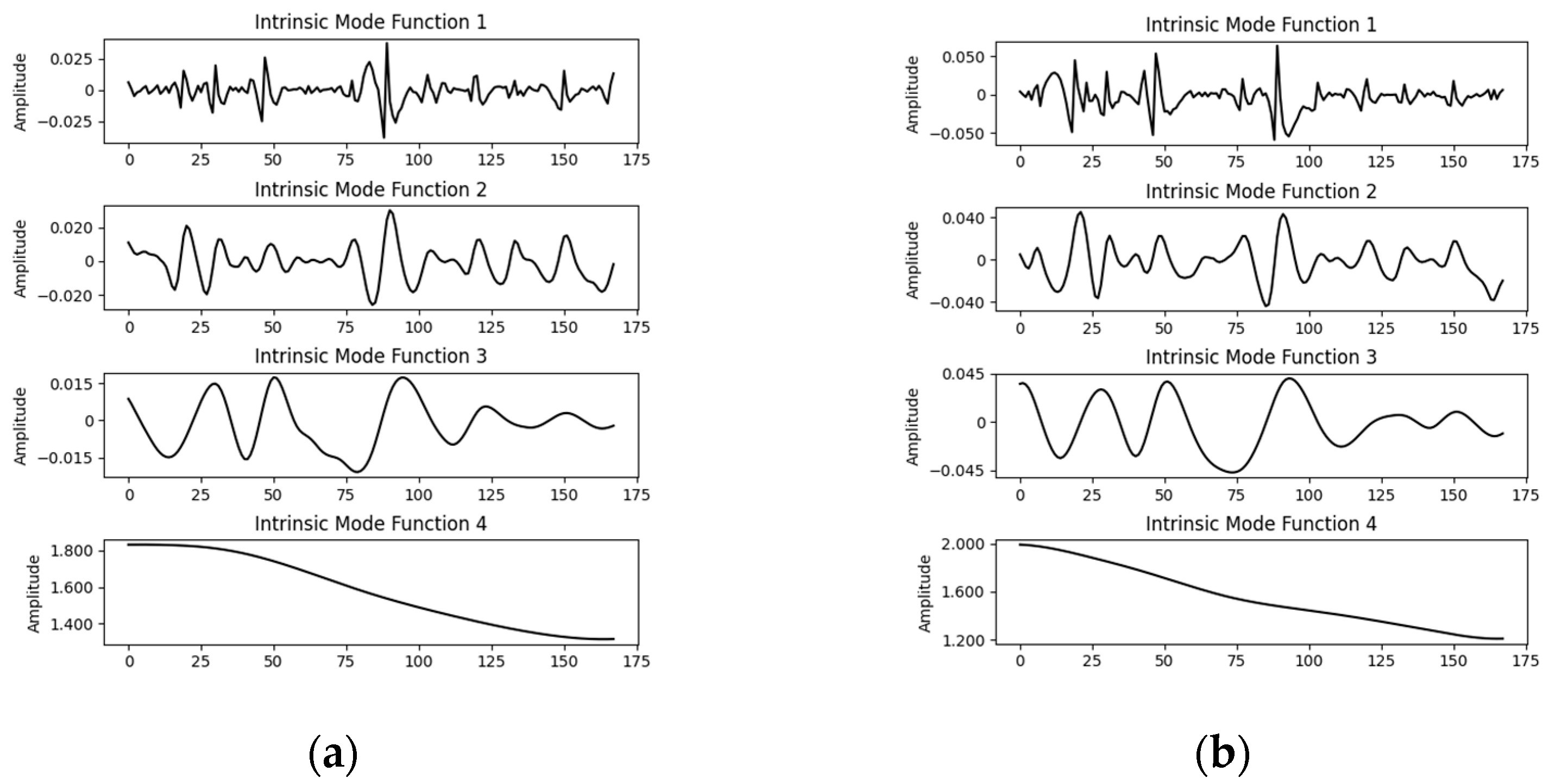
The battery capacity data were decomposed via CEEMDAN. Figure 7a,b show the capacity decomposition results for the B0005 and B0006 batteries, respectively. During the experiment, the two battery capacity datasets were decomposed into four IMFs. The IMFs were calculated by the RF fitting degree. The original volume data were verified to have good explanatory ability. IMF4 is the trend item, and the other IMFs, IMF1 to IMF3, are high-frequency components. These components contain noise but also contain some real information.

3.4. IMF Weight Calculation

RF is an ensemble learning method proposed by Leo Breiman in 2001 [33]. The core idea of RF is to construct multiple decision trees and aggregate their prediction results to improve the accuracy and stability of the model. As a nonlinear nonparametric method, RF can effectively weigh the contribution of each feature to the target variable. In the IMF analysis after modal decomposition, the importance ranking and value of each IMF were obtained via the RF as the weight of each IMF on the original data.

IMF1 to IMF4 of each battery were used as feature variables, and the original data were used as response variables to perform variable weight and fitting degree calculations via RF. IMF4 is a low-frequency trend term; therefore, the weight is fixed at 1 [22]. The weight coefficients of each high-frequency fluctuation component calculated from these values are shown in

Table 5. Random forest regression results.

Battery No.	IMF1	IMF2	IMF3	Degree of Fit
B 0005	0.023	0.063	0.115	0.999346
B 0006	0.074	0.036	0.122	0.999161
B 0007	0.031	0.093	0.080	0.993288
B 0018	0.025	0.043	0.173	0.994069

.

The fitting scores of the four batteries are all above 99%, indicating that the decomposed IMF has good interpretability for the original data. Prediction results for each IMF are reconstructed via the weights of a RF to obtain an estimate of the original data. This method not only avoids the impact of noise in the data on the model prediction ability but also does not completely abandon the feature information in the high-frequency component, thus improving the prediction accuracy of the model.

3.5. MHA-ED-LSTM Neural Network

3.5.1. LSTM Neural Network

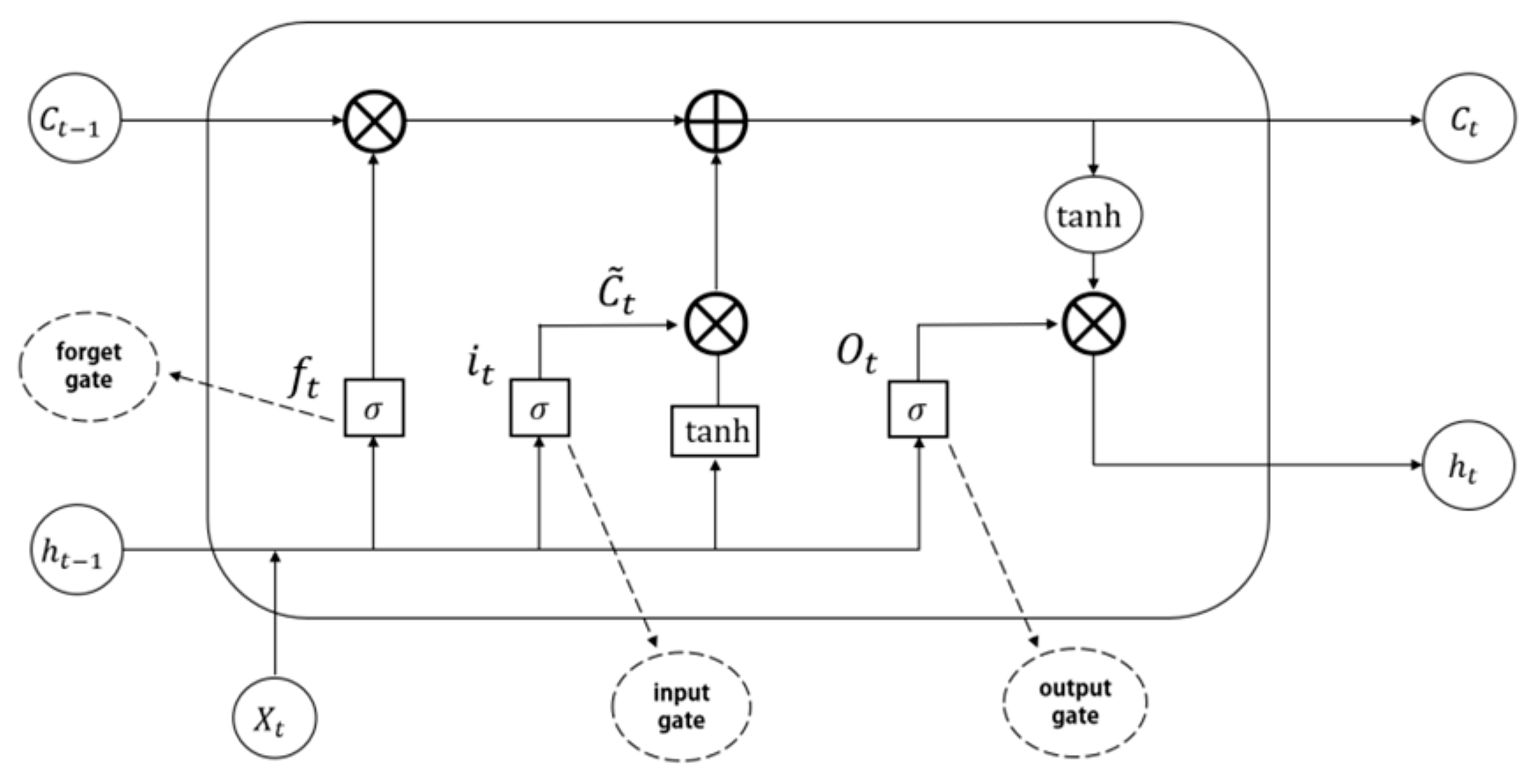
The LSTM consists of a forget gate, an input gate, and an output gate. These gates are responsible for updating or discarding historical information, enabling the LSTM to possess the capability of long-term memory [34]. Figure 8 shows the structure diagram of LSTM.

The principle formula is as follows:

$$f_t=\sigma (W_f·\left[h_{t-1},x_t\right]+b_f)$$

(5)

$$i_t=\sigma (W_i·\left[h_{t-1},x_t\right]+b_i)$$

(6)

$$\widetilde{C_t}=tanh(W_c·\left[h_{t-1},x_t\right]+b_c)$$

(7)

$$C_t=(f_t·C_{t-1}+i_t·\widetilde{C_t})$$

(8)

$$O_t=\sigma (W_o·\left[h_{t-1},x_t\right]+b_o)$$

(9)

$$h_t=O_t·tanh\left(C_t\right)$$

(10)

where $x_t$ and $h_t$ are the input and hidden states corresponding to time t, respectively; $f_t$, $i_t$ and $O_t$ are the states of the forget gate, the input gate and the output gate, respectively; $\widetilde{C_t}$, $C_t$ and $h_t$ are the states of the neuron and unit to be updated, respectively; $W_f$, $W_i$, $W_c$ and $W_o$ and $b_f$, $b_i$, $b_c$, and $b_o$ are the weight matrix and bias term of each gate, respectively; $\sigma$ and tanh are the activation functions.

3.5.2. Encoder-Decoder Structure

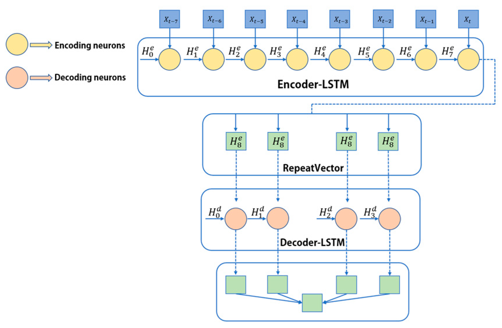
The ED structure consists of two main parts: an encoder and a decoder. Figure 9 shows the ED-LSTM structure constructed by using the LSTM neural network in this paper. The basic idea is to use an LSTM as an encoder to gradually process each element in the input sequence and update its internal state. The internal state at the last time step is considered a compressed representation of the entire input sequence, which is a fixed-length context vector. This vector is repeated multiple times and is used as the initial input of another LSTM that acts as a decoder. At each time step, the decoder’s output at the current time step is generated on the basis of the output at the previous time step, the current hidden state and the context vector. In the time series prediction task, when the input sequence is too long and contains more information, the LSTM can effectively memorize the long-term dependent information through its special gating mechanism, and the ED-LSTM structure constructed via the LSTM neural network can be more accurate. It captures the complex patterns and nonlinear relationships in the input sequence well and has stronger expressive ability and flexibility.

3.5.3. Multi-Head Attention Mechanism

This work introduces an attention mechanism after the ED structure to improve the model’s ability to capture contextual information. By connecting attention, the model assigns corresponding weights to each part of the input sequence to focus on the key information and better capture the dependency relationships between sequences [35]. To further improve the training efficiency and expressive ability of the model, the input is segmented into multiple heads, and the attention is calculated in parallel in multiple subspaces so that the model can capture and integrate different aspects of context information simultaneously.

The operational formula of the MHA mechanism is as follows:

$$MultiHead(Q,K,V)=Concat[{head}_1,{head}_2,\cdots {head}_p]W^G$$

(11)

$${head}_p=Attention(Q_p,K_p,V_p)$$

(12)

$$Attention\left(Q,K,V\right)=softmax\left({\displaystyle \frac{Q{K}^T}{\sqrt{d_k}}}\right)V$$

(13)

where Q, K, and V represent the query, key and value matrices, respectively.$W^G$ represents a trainable weight matrix; p represents the number of heads; attention represents the attention mechanism; and $d_k$ represents the number of columns of the K matrix, that is, the dimension of the vector.

3.6. Framework of Prediction Methods

The IMF obtained from the CEEMDAN decomposition of the nonlinear battery capacity data can represent the original data to different degrees, and different weights are assigned via the RF. The encoder–decoder structure in the ED-LSTM neural network can effectively capture the context information of the input sequence, whereas the LSTM can effectively capture the long-term dependency through its special gating mechanism. MHA can help to better capture the global characteristics of data and enhance the ability to model the intrinsic structure of complex data. Therefore, this paper proposes an RUL prediction method that combines CEEMDAN, RF, ED-LSTM and MHA. Figure 10 shows the framework of the method, and the framework process contains four aspects.

(1) The capacity data were selected as the health factors reflecting the RUL degradation trend, and the capacity data were subjected to CEEMDAN decomposition to obtain N ${IMF}_i$. Each IMF was used as a feature variable, and the capacity data were used as a response variable. RF regression was performed to obtain the weight of each IMF;

(2) The LSTM was used to construct the ED model, and the MHA was introduced into this structure;

(3) Each ${IMF}_i$ was converted and used as the input to train the model. The PSO was used to optimize the model parameters by comparing the error indicators corresponding to the IMF with the highest weight under different model parameter combinations to obtain a more accurate neural network prediction model;

(4) In the prediction stage, the results obtained by each IMF in the model were weighted by the weights obtained from the RF to obtain the final estimated value, and then the evaluation indicators between the actual data and the actual data were calculated and used as the evaluation criteria for the performance of the predictive models.

3.7. Optimization of Model Parameters

Particle swarm optimization is a swarm behavior-based optimization method. This algorithm looks for the global optimal solution by simulating the group predation behavior of fish or birds. Zhi et al. [36] employs the GA-PSO algorithm to discover the ideal parameter values for the SVR. By integrating PSO with GA algorithm, the diversity of the PSO particles is enhanced, causing them to navigate towards a novel search domain. This enhances the algorithm’s convergence pace and prevents it from becoming trapped in local extrema.

The core mechanism of PSO iteratively updates the speed and position of a particle to gradually approach the global optimal solution. In PSO, each candidate solution is considered a “particle” in the solution space; within a given parameter range, each particle represents a set of hyperparameters for a neural network model, and its movement process represents the search activity in that space. In the search activity, the current position of the particle represents its corresponding solution, which is the current hyperparameter combination, its velocity is the speed and direction of particle movement in the search space, which affects its position update in the next iteration. The velocity update equation integrates the particle’s previous best solution and the swarm’s historical optimal solution to effectively guide the exploration of particles in the solution space. Through multiple iterations, the algorithm locates the optimal solution that meets the predetermined stopping criteria.

The velocity update formula is as follows:

$$v_{id}^{k+1}=\omega v_{id}^k+c_1{r}_1\left(p_{id,pbest}^k-x_{id}^k\right)+c_2{r}_2\left(p_{d,gbest}^k-x_{id}^k\right)$$

(14)

Location update formula:

$$x_{id}^{k+1}=x_{id}^k+v_{id}^{k+1}$$

(15)

where i represents the serial number of the particle, i = 1, 2…, N, N is the size of the particle swarm; d represents the serial number of the particle dimension, d = 1, 2…, D, D is the dimension of the particle; k represents the number of iterations;$\omega$ represents the weight scale; $c_1$ and $c_2$ represent the individual learning factor and group learning factor, respectively; $r_1$ and $r_2$ represent random numbers in the interval [0:1], which increases the randomness of the search; $v_{id}^k$ and $x_{id}^k$ represent the speed vector and position vector of particle i in the d-th dimension in the k-th iteration, respectively; $p_{id,pbest}^k$ represents the historical optimal position of particle i in the d-th dimension in the k-th iteration, that is, the optimal solution obtained by the i-th particle (individual) after the k-th iteration. $p_{d,gbest}^k$ represents the historical optimal position of the d-th dimension of the swarm in the k-th iteration, that is, the optimal solution in the entire particle swarm after the k-th iteration.

The neural network model was optimized via a PSO search for a given parameter combination. The number of particles was set to 4, and the maximum number of iterations of the algorithm was 16. The Epochs, Num_heads and Batch_size of the model were selected for parameter optimization. The upper and lower bounds of Epochs were set to 70 and 150, respectively, the upper and lower bounds of Num_heads were set to 2 and 8, respectively, and the upper and lower bounds of Batch_size were set to 8 and 24, respectively. Within this parameter search range, the optimal parameter combination for each dataset searched by the PSO is shown in

Table 6. Optimal parameter combinations for each dataset.

Parameter	B 0005	B 0006	B 0007	B 0018
Epochs	90	82	94	124
Num_heads	6	4	8	6
Batch_size	8	8	23	14

.

4. Conclusions

In this paper, a CEEMDAN-RF-MHA-ED-LSTM lithium–ion battery RUL prediction method was proposed, and the NASA experimental dataset was selected to validate the reliability of the method. The following conclusions were drawn:

(1) The battery was affected by various uncertain factors during the working process, so the collected data contain a large amount of noise and fluctuations. High-frequency dynamic and nonlinear capacity curves prevent the model from accurately learning battery capacity fading characteristics. Therefore, CEEMDAN was used to perform noise reduction on original data. The predicted results show that the results obtained by decomposing the data through CEEMDAN and then using a neural network model for prediction have lower errors compared to the results obtained by using a neural network model alone. For example, on the No. 05 battery dataset, the mean absolute error, root mean square error, mean absolute percentage error, and relative error of the CEEMDAN-ED-LSTM method are 34%, 32%, 32% and 50% lower than those of the ED-LSTM method, respectively. The mean absolute error, root mean square error, mean absolute percent error and relative error of the CEEMDAN-MHA-ED-LSTM method decreased by 26%, 27%, 27% and 86%, respectively, compared with those of the MHA-ED-LSTM method.

(2) In this time series forecasting task, MHA was introduced to the ED-LSTM to enable the model to better capture the dependency relationship and further reduce the forecast error. For example, on the No. 05 battery dataset, the mean absolute error, root mean square error, mean absolute percent error and relative error of the MHA-ED-LSTM method were 25%, 23%, 25% and 34% lower than those of the ED-LSTM method, respectively. Moreover, on the No. 06 battery dataset, the mean absolute error, root mean square error, mean absolute percentage error, and relative error of the MHA-ED-LSTM method are 22%, 23%, 22% and 45% lower than those of the ED-LSTM method, respectively.

(3) The weights of each IMF were obtained via the RF algorithm. After the final forecast results were adjusted by weights, the accuracies of the four sets of error indicators, namely, the MAE, RMSE, MAPE, and RE, were compared, and the accuracy of the majority of them was better than the accuracy of the method using only the CEEMDAN+ neural network. For example, in the No. 05 battery dataset, the MAE, RMSE, and MAPE of the CEEMDAN-RF-MHA-ED-LSTM method compared with those of the CEEMDAN-MHA-ED-LSTM method decreased by 10%, 5%, and 9%, respectively.

(4) Based on the PSO algorithm, the weight of each IMF was obtained via RF, and the error indicators of the IMF with the highest weight proportion under different model parameter combinations are compared for model parameter optimization. After optimizing the parameters of the model, its error index further decreased. Compared with those of the model without parameter optimization, the mean absolute error, root mean square error, mean absolute percent error and relative error on the No. 05 battery dataset decreased by 20%, 23%, 20% and 63%, respectively.

In summary, the CEEMDAN-RF-MHA-ED-LSTM method has higher RUL prediction accuracy than the other methods do, and it provides a reference for existing research on RUL prediction for lithium batteries.