Hybrid Deep Learning Approach for Fractional-Order Model Parameter Identification of Lithium-Ion Batteries

Abstract

Fractional-order models (FOMs) have been recognized as superior tools for capturing the complex electrochemical dynamics of lithium-ion batteries, outperforming integer-order models in accuracy, robustness, and adaptability. Parameter identification (PI) is essential for FOMs, as its accuracy directly affects the model’s ability to predict battery behavior and estimate critical states such as state of charge (SOC) and state of health (SOH). In this study, a hybrid deep learning approach has been introduced for FOM PI, representing the first application of deep learning in this domain. A simulation platform was developed to generate datasets using Sobol and Monte Carlo sampling methods. Five deep learning models were constructed: long short-term memory (LSTM), gated recurrent unit (GRU), one-dimensional convolutional neural network (1DCNN), and hybrid models combining 1DCNN with LSTM and GRU. Hyperparameters were optimized using Optuna, and enhancements such as Huber loss for robustness to outliers, stochastic weight averaging, and exponential moving average for training stability were incorporated. The primary contribution lies in the hybrid architectures, which integrate convolutional feature extraction with recurrent temporal modeling, outperforming standalone models. On a test set of 1000 samples, the improved 1DCNN + GRU model achieved an overall root mean square error (RMSE) of 0.2223 and a mean absolute percentage error (MAPE) of 0.27%, representing nearly a 50% reduction in RMSE compared to its baseline. This performance surpasses that of the improved LSTM model, which yielded a MAPE of 9.50%, as evidenced by tighter scatter plot alignments along the diagonal and reduced error dispersion in box plots. Terminal voltage prediction was validated with an average RMSE of 0.002059 and mean absolute error (MAE) of 0.001387, demonstrating high-fidelity dynamic reconstruction. By advancing data-driven PI, this framework is well-positioned to enable real-time integration into battery management systems.

1. Introduction

1.1. Literature Review

Fractional-order models (FOMs) have emerged as a powerful tool for accurately capturing the complex electrochemical dynamics of lithium-ion batteries, offering significant improvements over traditional integer-order models in terms of accuracy, robustness, and adaptability to varying operating conditions [1,2,3]. Parameter identification (PI) is a critical step in leveraging the full potential of FOMs, as it directly impacts the model’s ability to predict battery behavior, estimate state of charge (SOC), and assess state of health (SOH) [4,5]. Accurate PI is crucial for the deployment of FOMs in battery management systems (BMS) and hybrid energy storage systems [6,7]. Reliable model parameters are preconditions for high-precision state estimation, such as State of Charge (SOC) [8]. The core challenge in identifying FOM parameters lies in the inherent nonlinearity introduced by the fractional order, which distinguishes them from integer-order models (IOMs). The model parameters and the fractional order are highly sensitive and time-varying, depending on numerous factors such as SOC, temperature, SOH, and load.

FOM parameter identification methods are generally categorized by their operational domain (frequency vs. time) and implementation style (offline vs. online/recursive). Offline and global optimization methods are particularly favored for identifying parameters in complex, non-convex problems due to their robust global search capabilities, which help avoid convergence to local minima. Among the intelligent optimization algorithms employed, particle swarm optimization (PSO) is widely used, often enhanced through variants such as hybrid multi-swarm PSO [9] or by incorporating chaos theory to refine local search [10]. Further improvements include adaptive fractional order PSO, which dynamically adjusts a particle’s inertia weight based on its proximity to the global optimum [11]. Coevolutionary PSO (CPSO) has also been applied to synchronously identify both the parameters and the order-values of FOMs [12,13]. Genetic algorithm (GA) and its hybrid with PSO are also utilized for the simultaneous identification of model coefficients and differentiation orders [9,14,15]. For instance, the hybrid genetic–fractional beetle swarm optimization method, which synergizes GA with fractional beetle swarm optimization, has demonstrated superior accuracy compared to individual algorithms [16]. Additionally, variants of differential evolution (DE), such as the neighborhood-based multi-strategy and mean factor DE algorithm, are designed to enhance population diversity and convergence performance [17]. Beyond these, the Runge–Kutta optimizer (RUN) is also utilized, leveraging its fast convergence speed and high precision for extracting FOM parameters from either electrochemical impedance spectroscopy (EIS) or time-domain data [18].

For real-time applications requiring rapid parameter tracking under varying operating conditions, online and adaptive methods are essential. The forgetting factor recursive least squares (FFRLS) algorithm is commonly employed for the fast online identification of linear model parameters when the fractional order is predetermined [19,20], utilizing discrete representations of the fractional derivative such as the Grünwald–Letnikov definition [6,15,21,22]. To address the simultaneous identification of all parameters including the fractional order α, multi-time scale frameworks have been proposed. In such frameworks, α is updated periodically on a slow time scale using global optimization methods with low computational burden, while remaining parameters are updated frequently via FFRLS on a fast time scale. Synergistic approaches, such as the beetle antennae search and recursive least squares (BAS-RLS), iteratively determine α using BAS while RLS estimates linear parameters [5]. Variable-order recursive methods repeatedly apply RLS with different fractional orders to continuously correct approximation errors and converge toward the optimal dynamic order [20]. Kalman Filter-based integration, including the adaptive extended Kalman filter (AEKF) and adaptive fractional-order unscented particle filter, simultaneously estimates state-of-charge, state-of-health, and model parameters by treating them as part of an extended state vector [23,24]. Gradient Descent variants, such as weighted gradient descent and weighted forgetting factor gradient descent, are also utilized for online identification of both parameters and fractional orders, incorporating weighting factors inspired by particle filter innovations to enhance precision and convergence speed [22]. Multi-domain identification strategies combine optimization in both time and frequency domains, constructing a unified objective function to achieve parameter sets that satisfy both impedance characteristics and dynamic response simultaneously. Algorithms such as GA-PSO are typically employed for this multi-domain optimization [15]. Furthermore, data-driven techniques like transfer learning combined with back propagation neural networks (BPNN) have been applied to accurately identify physics-based FOM parameters across the battery’s entire life cycle, demonstrating effectiveness even under accelerated aging conditions [25].

Table 1. Comparison of various parameter identification methods.

Category	Typical Methods/Algorithms	Advantages	Disadvantages
I. Offline Global Optimization	PSO, GA, DE, RUN, CPSO	Guaranteed ability to search for the global optimum solution, essential for finding the inherently nonlinear fractional order (α). High resulting model accuracy (low RMSE/MAE).	High computational complexity and expense, unsuitable for real-time/on-board applications due to batch processing requirement.
II. Online Recursive (Decoupled/Fixed Order)	RLS, FFRLS, AEKF	Low computational load, fast parameter updates suitable for real-time/microprocessor implementation. Effective for tracking linear parameters.	Requires α to be fixed or determined separately, which may lead to parameter estimation errors and loss of physical meaning.
III. Online Adaptive	BAS-RLS	Realizes simultaneous full-parameter and order identification online, capturing dynamic changes in α. Provides highly accurate terminal voltage prediction.	Increased computational burden compared to fixed-order RLS methods, often requiring complex software implementation (e.g., G-L definition).
IV. Multi-Domain and Data-Driven	GA + PSO, Transfer Learning + BPNN	Improves robustness by constraining parameters across both frequency (EIS) and time (dynamic) domains. Data-driven methods facilitate parameter tracking across the entire aging lifecycle.	Requires extensive experimental data collection (both EIS and time-domain). Data-driven methods require a large training dataset for initial learning.

summarizes the advantages and disadvantages of the PI methods for FOM.

On the other hand, machine learning and deep learning (DL) are also applied to the parameter identification of equivalent circuit models of lithium-ion batteries as well as other complex systems. Techniques including long short-term memory (LSTM) networks, convolutional neural networks (CNNs), and hybrid models (e.g., CNN–LSTM) have demonstrated the capability to accurately estimate time-varying or uncertain parameters by extracting temporal and spatial features from measurement data, often outperforming traditional methods in terms of robustness and accuracy [26,27]. In scientific and engineering contexts, DL architectures are increasingly applied to inverse problems and PI in partial differential equations (PDEs), offering flexible solutions for both direct and indirect measurement scenarios [28,29]. Qiang You et al. present a machine learning approach to accurately identify parameters of the 11-dimensional adapted randles equivalent circuit model from EIS data, overcoming the high-dimensionality challenge by reducing the model into two low-dimensional forms and applying a Euclidean distance-based pre-classification to select optimal training data for Gaussian process regression [30]. In [31], a neural network is developed to estimate key physics-based electrochemical properties from equivalent circuit model (ECM) parameters, achieving prediction errors below 1% for electrolyte transport properties in nearly all cases. Hanjing Fu et al. present a novel physics-informed neural network (PINN) model that integrates an ECM within a recurrent neural network (RNN) framework for lithium-ion battery modeling and SOH estimation, achieving high accuracy with SOH errors below 2% [32]. Zeyang Geng et al. introduce a new implementation of Pseudo-Two-Dimensional (P2D) model using a transmission line circuit structure combined with the finite difference method, effectively bridging physics-based and equivalent circuit models to deliver precise results without relying on empirical fitting [33]. However, the application of DL to PI remains relatively underexplored in certain domains. For instance, Junfu Li et al. [34] developed a DL method using CNNs for online PI in Lithium-ion batteries; however, the inputs to their model were preprocessed features rather than raw data, and the electrochemical model employed is relatively complex and not well-suited for BMS applications. Zichen Du and Renhao Lu review the use of physics-informed neural networks (PINNs) for efficient thermal management in electronics and battery systems, highlighting their speed and accuracy compared to traditional methods. It discusses recent advancements, challenges, and future research directions for integrating PINNs with advanced technologies [35]. In previous work, the authors proposed a DL approach for PI of a 2RC ECM [36]. To the best of the authors’ knowledge, no study has yet applied DL to PI of a FOM. Therefore, this paper introduces several DL models to estimate the parameters of FOMs, aiming to validate their feasibility and effectiveness in this emerging area.

1.2. Theoretical Backgrounds

The methodologies employed in this study encompass various deep learning techniques and their improvement methods. To facilitate understanding, the theoretical foundations and implementation principles of each method—spanning LSTM, gated recurrent unit (GRU), and one-dimensional convolutional neural network (1DCNN)—as well as improvement techniques including the Huber loss function, stochastic weight averaging (SWA), and exponential moving average (EMA), are introduced as follows.

1.2.1. LSTM and GRU [37]

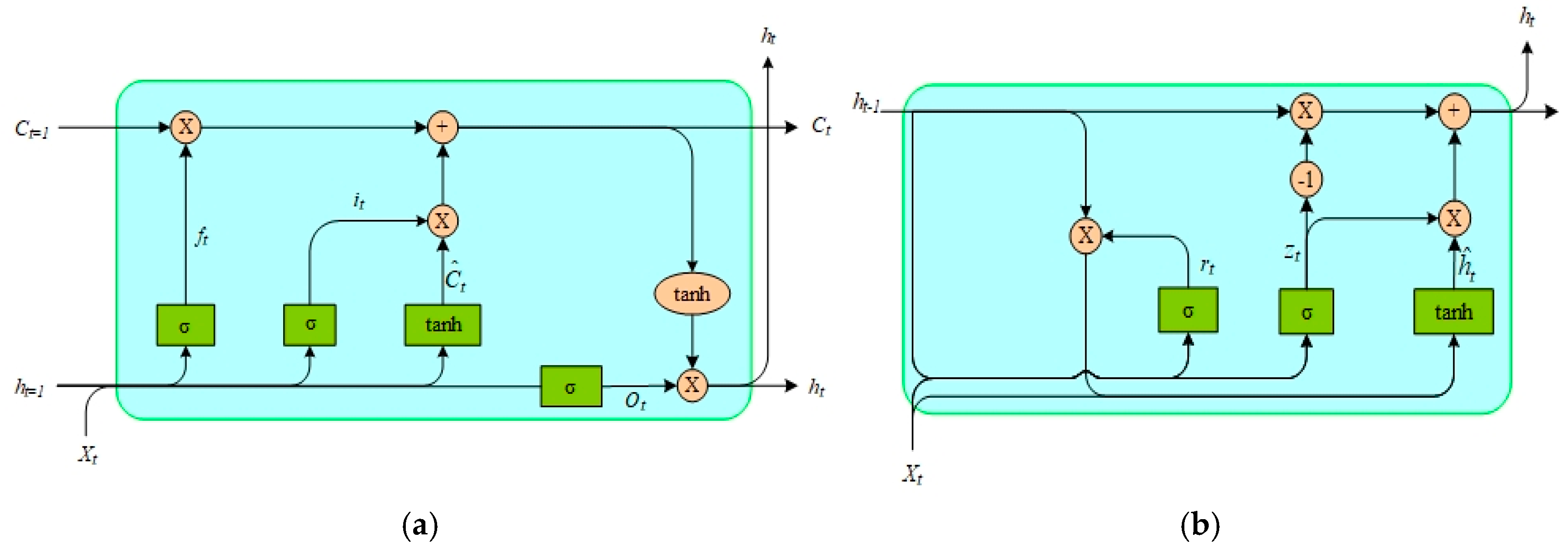
LSTM and GRU were employed as advanced recurrent neural network architectures to handle sequential data, leveraging their ability to capture long-term dependencies. The LSTM cell diagram revealed a structure with three gates as shown in Figure 1a: the forget gate $f_t$, input gate $i_t$, and output gate $o_t$, alongside a cell state $C_t$ and hidden state $h_t$. Mathematically, the LSTM operations were defined as follows: the forget gate output was $f_t=\sigma \left(W_f·[h_{t-1},x_t]+b_f\right)$, the input gate output was $i_t=\sigma \left(W_i·[h_{t-1},x_t]+b_i\right)$, the cell candidate was ${\tilde{C}}_t=\mathit{tanh}\left(W_c·[h_{t-1},x_t]+b_c\right)$, the cell state update was $C_t=f_t·C_{t-1}+i_t·{\tilde{C}}_t$, and the hidden state was $h_t=o_t·\mathit{tanh}\left(C_t\right)$ with $o_t=\sigma \left(W_o·[h_{t-1},x_t]+b_o\right)$. This allowed LSTM to selectively remember or forget information over time, making it suitable for the time-series problem where long-term patterns were critical. The GRU cell diagram shown in Figure 1b simplified the architecture with two gates: the reset gate $r_t$ and update gate $z_t$, merging the forget and input gates into a single update mechanism. The GRU equations were $r_t=\sigma \left(W_r·[h_{t-1},x_t]+b_r\right)$, $z_t=\sigma \left(W_z·[h_{t-1},x_t]+b_z\right)$, the candidate hidden state was ${\tilde{h}}_t=\mathit{tanh}\left(W·[r_t·h_{t-1},x_t]+b\right)$, and the hidden state update was $h_t=(1-z_t)·h_{t-1}+z_t·{\tilde{h}}_t$. This reduction in complexity improved computational efficiency while retaining the ability to model dependencies, which was advantageous for the problem. Both LSTM and GRU models were suitable for this problem because of their intrinsic ability to model long-range dependencies, a requirement directly analogous to the memory effect observed in lithium-ion battery dynamics. The battery’s voltage response is governed by its entire historical usage, an enduring non-local effect that standard RNNs could not capture due to the vanishing gradient. By regulating the information flow through their respective gating mechanisms, LSTM and GRU were enabled to maintain a persistent internal state (memory) over extended time steps. This effectively allowed the models to learn the complex, nonlinear patterns within the sequential battery data and implicitly capture the same long-memory behavior that was explicitly represented by the fractional-order elements (like CPE and Warburg) in the analytical FOMs.

1.2.2. DCNN [38]

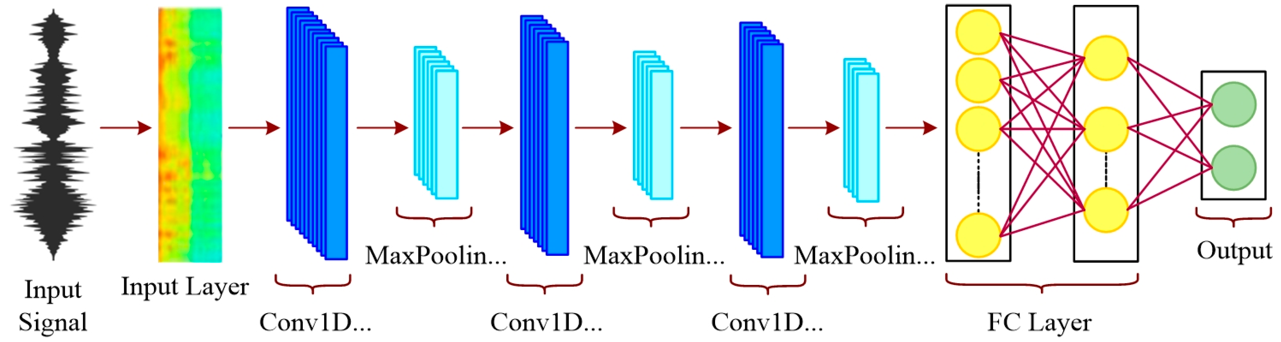
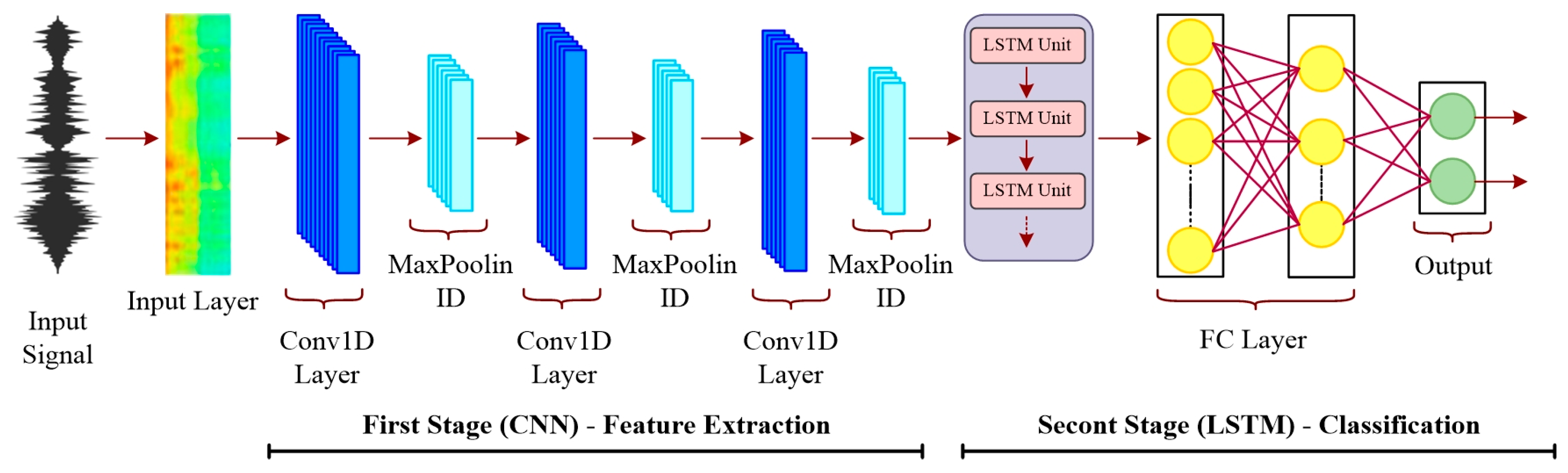
The 1DCNN was utilized as an effective architecture for processing the sequential time-series data from the battery. Unlike 2D CNNs, which slide filters across two spatial dimensions, the 1DCNN employed filters that were moved exclusively across the single time dimension of the input vector (the “Input Signal”). This design allowed the network to automatically extract crucial features regardless of their position in the sequence. As illustrated in Figure 2, the fundamental operation of a 1DCNN is the convolution performed in layers like ‘Conv1D Layer’. In this process, a small filter (kernel), $K$, was applied to a localized segment of the input sequence, $X$, at time step $t$ to produce an element in the output feature map, $y_t$. This operation was mathematically defined by:

$$y_t=f\left({\displaystyle \sum _{i=0}^{N-1}{K}_i}·X_{t+i}+b\right)$$

(1)

where N is the kernel size, b is the bias, and $f$ is the nonlinear activation function. This filter was swept across the entire input sequence, generating a feature map that highlighted specific temporal patterns. Following the convolutional layer, a Max Pooling 1D layer was typically applied to reduce the dimensionality of the feature maps, thereby decreasing computational load and making the model more robust to minor temporal shifts. The resulting high-level feature maps were then flattened and passed to a fully connected layer (FC Layer) for the final prediction.

The 1DCNN was employed for this problem because of its efficacy in processing time-series data. The convolutional filters were adept at automatically identifying local temporal features within the sequences, such as sharp current pulses or rapid voltage transients, which are crucial signatures of internal battery kinetics (e.g., Ohmic and charge-transfer resistances). Since the filters were shared across the entire length of the sequence, the model was made translationally invariant, meaning it could detect a specific transient feature regardless of where it appeared in the operating cycle. Furthermore, the 1DCNN generally had a lower computational cost for feature extraction compared to recurrent models, and it demonstrated superior capability in extracting the essential, localized features from the input sequences, a factor which subsequently justified its incorporation into the hybrid architectures to enhance overall predictive power.

1.2.3. Improvement Strategies

Two improvement strategies, the adoption of the Huber loss function [39] and the implementation of SWA [40] and EMA [41], are incorporated to further enhance the robustness and generalization performance of the proposed deep learning models. Next, the theoretical basis of these technologies will be introduced.

The Huber loss function is a robust regression metric that combines the squared error for small residuals and the absolute error for large ones, defined as

$${\mathrm{L}}_{\delta }(y,\widehat{y})=\left\{\begin{array}{c}{\displaystyle \frac{1}{2}}{(y-\widehat{y})}^2,if\left|y-\widehat{y}\right|\le \delta \\ \delta (\left|y-\widehat{y}\right|-{\displaystyle \frac{1}{2}}\delta ),otherwise\end{array}\right.$$

(2)

where d is a tuning parameter. This formulation mitigates the influence of outliers compared to mean squared error while retaining sensitivity to smaller errors.

SWA is a training technique that improves generalization by averaging the weights of a model visited during the later stages of stochastic gradient descent optimization, resulting in a flatter minimum in the loss landscape. Mathematically, the averaged weights are computed as

$${\theta }_{\mathrm{SWA}}={\displaystyle \frac{1}{N}}{\displaystyle \sum _{i=1}^N{\theta }_i}$$

(3)

where ${\theta }_i$ denotes the model weights at the $i^{th}$ checkpoint and $N$ is the total number of checkpoints used for averaging. By averaging these parameters, SWA effectively shifts the final solution toward the center of a wider and flatter region in the loss landscape. This property reduces the model’s sensitivity to local fluctuations and improves its generalization capability under varying data distributions. In practice, SWA was applied during the last 20–30% of training epochs, allowing the optimizer to converge to a stable region before averaging began.

EMA keeps a running (exponentially decaying) average of past parameter values, giving recent weights the highest influence and producing a smoother, more stable parameter estimate. The update rule for EMA is defined as

$${\theta }_{\mathrm{EMA}}^{(t)}=\beta ·{\theta }_{\mathrm{EMA}}^{(t-1)}+(1-\beta )·{\theta }^{(t)}$$

(4)

where ${\theta }^{(t)}$ represents the current model weights and $\beta \in [0.999,0.9995]$ is the exponential decay factor controlling the smoothing strength. EMA acts as a low-pass filter, damping high-frequency noise caused by stochastic gradient variations, thus ensuring a smoother and more stable convergence trajectory. By combining both techniques during the final fine-tuning stage, the model benefits from the complementary effects of discrete checkpoint averaging (SWA) and continuous weight smoothing (EMA).

1.3. Contributions of the Proposed Method

In this study, a simulation platform for the FOM of lithium-ion batteries is first established. The platform is used to generate training and testing datasets through two different sampling strategies: Sobol sampling and Monte Carlo sampling. Subsequently, this work addresses the PI problem of the FOM by developing three DL-based identification frameworks, namely LSTM, GRU, and 1DCNN. The hyperparameters and architectures of these models are optimized using Optuna (version 4.5.0), and their performances are systematically compared. In general, DL models generally exhibit superior representation and generalization capabilities compared to traditional methods, as they learn nonlinear relationships directly from data without necessitating explicit mathematical modeling or manual feature extraction. In contrast, optimization-based techniques such as PSO, GA, or RLS rely on iterative search procedures and often incur substantial computational costs, particularly for high-dimensional or fractional-order systems. Moreover, the trained hybrid deep network enables parameter identification through a single forward pass, significantly reducing inference time while maintaining competitive or enhanced accuracy. The hybrid CNN-GRU framework presents a clear advantage over conventional feature-based machine learning approaches by obviating the need for manual feature engineering and selection. Traditional methods, including tree-based models and support vector machines, rely heavily on domain expertise to extract and predefine salient input features, whereas the deep learning architecture autonomously learns hierarchical and temporal features directly from raw data. This data-driven approach not only mitigates human bias but also facilitates the discovery of complex nonlinear patterns that may be overlooked by manual processes, resulting in a more robust and generalizable model for identifying intricate system parameters. The neuro-physical approach, which incorporates physical laws as constraints within neural network architectures, can indeed be extended from traditional ECMs to FOMs to enhance physical consistency. However, the proposed hybrid deep learning method fundamentally differs by adopting a data-centric rather than a physics-informed strategy. While neuro-physical methods require explicit and accurate prior knowledge of governing equations, our approach exploits the representational capacity of deep learning to implicitly capture complex dynamics directly from data. This confers a significant advantage for FOMs, where governing fractional-order operators are often computationally intensive or where the underlying physical processes are not fully characterized, thereby offering greater flexibility and the potential to uncover unmodeled dynamics.

In this study, two hybrid architectures—1DCNN + LSTM and 1DCNN + GRU—are proposed to enhance the identification accuracy by leveraging both temporal dependency learning and feature extraction capabilities. Finally, two improvement strategies are introduced to further enhance the performance and generalization ability of the DL models: (1) adopting the Huber loss function to achieve a balance between robustness and sensitivity to outliers, and (2) SWA, and EMA have been applied to improve robustness and training stability. Performance on a 1000-sample test set has been evaluated using root mean square error (RMSE) and mean absolute percentage error (MAPE), with scatter plots, box plots, and heatmaps utilized to assess accuracy for parameters. The improved 1DCNN + GRU model has been identified as the top performer, achieving an RMSE of 0.2223 and MAPE of 0.27%. Terminal voltage prediction has also been validated, yielding an average RMSE of 0.002059 and mean absolute error (MAE) of 0.001387, thereby confirming the models’ ability to reconstruct dynamic battery behavior with high fidelity. This study employs a data-driven framework where DL models are trained on simulated synthetic data. Once trained, these models can be directly deployed onto a digital signal controller for real-time, online parameter identification. The main contributions of this paper are listed as follows:

• DL has been applied innovatively to FOM PI problem for lithium-ion batteries, addressing gaps where traditional methods like PSO or RLS are constrained by computational demands or inability to manage nonlinear fractional orders in real-time.
• Hybrid architectures have been introduced, combining convolutional local feature extraction with recurrent temporal modeling, resulting in superior performance; for example, the improved 1DCNN + GRU reduces overall RMSE by nearly 50% from baseline (0.4386 to 0.2223) and achieves MAPE of 0.27%, outperforming the improved LSTM’s 9.50% MAPE.
• A simulation platform has been established for dataset generation via Sobol and Monte Carlo strategies, providing diverse and representative data without reliance on physical experiments, thus facilitating scalable training; hyperparameters have been optimized using Optuna to ensure comparative fairness.
• Two enhancement strategies have been proposed: Huber loss for balancing robustness against outliers and sensitivity, and SWA with EMA for training stabilization, leading to up to 31-fold RMSE improvements in hybrids (e.g., 1DCNN + LSTM from 4.658 to 0.268); these are reflected in heatmaps showing consistent low errors across parameters.
• Terminal voltage prediction has been validated with average RMSE of 0.002059 and MAE of 0.001387, enabling high-fidelity reconstruction of battery dynamics and advancing practical applications in BMS by supporting adaptive PI under varying conditions.

2. Fractional-Order Model of Lithium-Ion Batteries

2.1. Brief Description of Fractional-Order Model

An FOM of a lithium-ion battery is an evolution of traditional modeling techniques that leverages fractional calculus (differentiation and integration to a non-integer order) to more accurately describe the complex, non-ideal dynamics within the cell. Instead of relying only on ideal integer-order components like pure resistors and capacitors, the FOM introduces elements that capture the distributed and dispersive nature of electrochemical processes. The model’s key components, which replace or enhance those in standard ECM, include the constant phase element (CPE) and the fractional-order Warburg element. The CPE is used to model non-ideal capacitance, particularly the double-layer capacitance at electrode-electrolyte interfaces. In a real battery, the electrode surface is not perfectly smooth; its roughness and porosity cause a distribution of relaxation times. An ideal capacitor has an impedance with a phase angle of −90°, while a resistor has a phase of 0°. The CPE’s impedance shown in Equation (5) has a constant phase angle between 0° and −90°

$$Z_{\mathrm{CPE}}(\omega )={\displaystyle \frac{1}{Q{(j\omega )}^{\alpha }}}$$

$$Z_{\mathrm{Re}}={\displaystyle \frac{1}{Q{\omega }^{\alpha }}}\mathit{cos}\left({\displaystyle \frac{\alpha \pi }{2}}\right),Z_{\mathrm{Im}}=-{\displaystyle \frac{1}{Q{\omega }^{\alpha }}}\mathit{sin}\left({\displaystyle \frac{\alpha \pi }{2}}\right),0<\alpha <1$$

(5)

where Z_CPE is the impedance of the CPE, Q is the CPE coefficient determining magnitude. α is the fractional order (0 < α < 1): α = 1 yields a pure capacitor, α = 0 yields a pure resistor. ω is the angular frequency. j denotes the imaginary unit. The impedance comprises real (Z_Re) and imaginary (Z_Im) parts, representing resistive and capacitive contributions, respectively.

The fractional-order Warburg element models the diffusion of lithium ions within the solid electrode particles and the electrolyte. In a conventional analysis, the Warburg element for semi-infinite diffusion is an impedance as shown in Equation (6)

$$Z_W(\omega )={\displaystyle \frac{1}{W{(j\omega )}^{\alpha }}},\alpha =0.5$$

(6)

which corresponds to a fractional order of $\alpha =0.5$ and appears as a 45° line on a Nyquist plot. In lithium-ion batteries, a finite-length Warburg element is typically used to represent diffusion within a bounded volume (e.g., electrode particles).

The primary advantage of FOMs over ECM is significantly higher accuracy with comparable or even fewer fitting parameters. ECMs, like the common RC models, often require a high number of RC pairs to accurately match experimental data, particularly EIS plots, which is computationally expensive and makes parameter identification challenging [42]. FOMs achieve high fidelity by capturing the frequency-dependent behavior using elements with non-integer orders, which inherently accounts for the distributed parameters resulting from non-uniform electrode structure. Compared to electrochemical models (EChMs) such as the pseudo two-dimensional model, the FOM offers a compelling trade-off between physical meaning and computational efficiency. EChMs are based on coupled PDEs and are highly accurate, but they are computationally intensive, making them unsuitable for real-time applications in a BMS. The FOM, by replacing complex diffusion and surface dynamics with fractional-order ODEs, maintains a strong link to the underlying physics while being fast enough for real-time control and state estimation. This superior balance is why FOMs are becoming an increasingly popular choice for advanced battery management.

2.2. FOM Utilized in This Study

In fractional models, circuits combine R, CPE, and Warburg in series/parallel to simulate battery voltage response under various loads. The primary objective of this paper is to validate the feasibility of identifying FOM parameters using voltage response time-series data from batteries. To achieve this, the R(RQ)W model as shown in Figure 3 is selected to represent the lithium battery. This model structure consists of a resistor (R₀) in series with a parallel combination of another resistor (R₁) and a constant phase element (CPE₁), which is then in series with a Warburg element (W). The R(RQ)W model is chosen for its effectiveness in capturing key battery dynamics. The R(RQ) segment effectively describes the charge transfer and double-layer effects, while the series Warburg element is crucial for modeling the solid-state diffusion processes within the battery. This combination provides a compact yet accurate representation, making it highly suitable for FOM parameter identification from time-domain voltage data. The impedance expression of the FOM used in this paper is given in Equation (7).

$$Z(s)=R_i+{\displaystyle \frac{R_1\frac{1}{s^{\alpha }{Q}_1}}{R_1+\frac{1}{s^{\alpha }{Q}_1}}}+{\displaystyle \frac{1}{s^{\beta }W}},0<\alpha <1,\beta =0.5$$

(7)

The model used in this paper is a fractional-order version of the popular Partnership for a New Generation of Vehicles (PNGV) model. The PNGV model accurately simulates battery behavior under dynamic loads, offering simplicity and good fit for hybrid vehicle applications. Converting it to a fractional-order representation enhances precision by better capturing nonlinear dynamics and memory effects, improving accuracy in modeling complex electrochemical processes with fewer parameters [43].

2.3. Time Domain Voltage Response of the Utilized FOM

Fractional calculus can be solved using methods like Grünwald-Letnikov (GL), Riemann-Liouville (RL), or Caputo. GL approximates fractional derivatives via discrete differences, suitable for numerical computations [44]. RL defines fractional integrals and derivatives through convolution, effective for analytical solutions. Caputo reformulates derivatives to handle initial conditions better, ideal for physical systems. GL method is often chosen for its straightforward numerical implementation and accuracy in discretizing fractional operators, especially in simulations. The R(RQ)W equivalent circuit is described by the following continuous-time state equations, with I(t) as the input current and $x(t)=\left[\begin{array}{c}{V}_1(t)\\ V_2(t)\end{array}\right]$ as the state vector:

$$\left\{\begin{array}{l}{D}^{\alpha }{V}_1(t)=-{\displaystyle \frac{1}{R_1{Q}_1}}{V}_1(t)+{\displaystyle \frac{1}{Q_1}}I(t)\hfill \\ D^{\beta }{V}_2(t)={\displaystyle \frac{1}{W}}I(t)\hfill \end{array}\right.$$

(8)

Here, D^a is the fractional derivative operator, a is the order of the CPE (Q), β is the order of the Warburg element (W) (typically β = 0.5), R₁Q₁ is the time constant of the RQ branch, respectively. For brevity, let $a_1=-{\displaystyle \frac{1}{R_1{Q}_1}},b_1={\displaystyle \frac{1}{Q_1}},a_2=0$, and $b_2={\displaystyle \frac{1}{W}}$.

The GL approximation is the core tool for discretization, as it transforms the fractional derivative at time $t_k=k\Delta t$ into a discrete, weighted sum that inherently captures the system’s long memory effect

$${\mathrm{D}}^{\alpha }x(t_k)\approx {\displaystyle \frac{1}{\Delta t^{\alpha }}}{\displaystyle \sum _{j=0}^k{c}_j^{(\alpha )}}{x}_{k-j}$$

(9)

where $\Delta t$ is the sampling time, and $c_j^{(\alpha )}$ are the GL coefficients, calculated recursively by $c_0^{(\alpha )}=1$ and $c_j^{(\alpha )}=\left(1-{\displaystyle \frac{\alpha +1}{j}}\right)c_{j-1}^{(\alpha )}$ for $j\ge 1$.

Applying the GL approximation to the state equations and solving for the state at the next time step, $V_{i,k+1}$, leads directly to the discrete state-space form. Use $j=0$ for the current state $V_{i,k+1}$ and move the memory terms (where $j\ge 1$) to the right side of the equation. The resulting discrete state-space equation for the $i^{th}$ state is:

$$V_{i,k+1}=\underset{{\tilde{A}}_{i,i}}{\underbrace{{\displaystyle \frac{-Q_1^{({\alpha }_i)}}{1-a_i{\Delta t}^{{\alpha }_i}}}}}{V}_{i,k}+\underset{{\tilde{B}}_i}{\underbrace{{\displaystyle \frac{b_i{\Delta t}^{{\alpha }_i}}{1-a_i{\Delta t}^{{\alpha }_i}}}}}{I}_{k+1}+\underset{{\tilde{\Gamma }}_{i,k}}{\underbrace{{\displaystyle \frac{-1}{1-a_i{\Delta t}^{{\alpha }_i}}}{\displaystyle \sum _{j=2}^{k+1}{c}_j^{({\alpha }_i)}}{V}_{i,k+1-j}}}$$

(10)

In the standard discrete state-space form, $x_{k+1}=A{x}_k+B{u}_{k+1}+{\Gamma }_k$:

$$x_{k+1}=\left[\begin{array}{c}{V}_{1,k+1}\\ V_{2,k+1}\end{array}\right]=\underset{A}{\underbrace{\left[\begin{array}{cc}{A}_{11}& 0\\ 0& A_{22}\end{array}\right]}}\left[\begin{array}{c}{V}_{1,k}\\ V_{2,k}\end{array}\right]+\underset{B}{\underbrace{\left[\begin{array}{c}{B}_1\\ B_2\end{array}\right]}}{I}_{k+1}+\underset{{\Gamma }_k}{\underbrace{\left[\begin{array}{c}{\Gamma }_{1,k}\\ {\Gamma }_{2,k}\end{array}\right]}}$$

(11)

The output equation for the terminal voltage $V_{t,k}$ is the sum of the open-circuit voltage $V_{oc,k}$, the ohmic drop, and the polarization voltages:

$$V_{t,k}=V_{oc,k}+V_{1,k}+V_{2,k}+R_0{I}_k \Rightarrow V_{t,k}=V_{oc,k}+\underset{C}{\underbrace{[11]}}{x}_k+\underset{D}{\underbrace{R_0}}{I}_k$$

(12)

This model is a concise Fractional-Order State-Space representation. The matrices $\mathrm{A}$ and $\mathrm{B}$ capture the immediate dynamics, while the crucial memory vector ${\mathsf{\Gamma }}_k$ (the long summation of past states weighted by GL coefficients) captures the long-term history dependence inherent to fractional-order systems, making the model highly accurate for real battery dynamics.

3. Description of the Proposed Parameter Identification Method

3.1. Description of the Generation of the Dataset

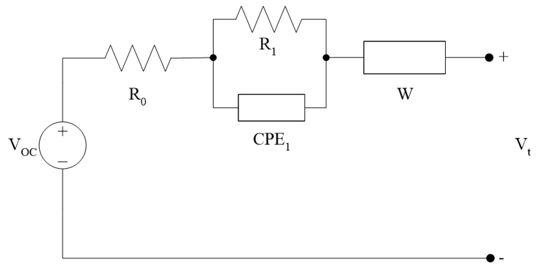
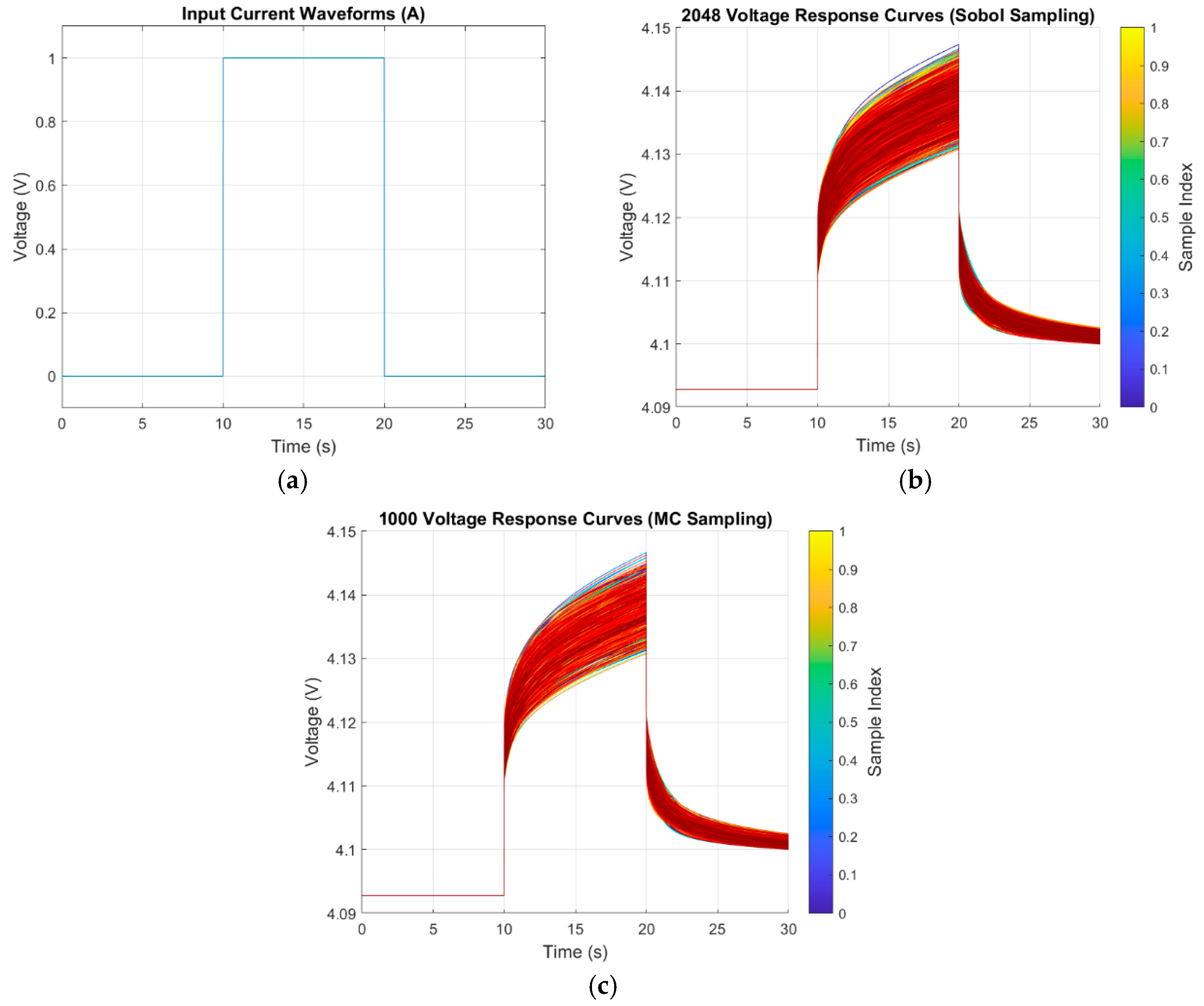
This study validates the feasibility of identifying FOM parameters from battery voltage response data, adopting the R(RQ)W model for its ability to capture key dynamics such as charge transfer and solid-state diffusion. A custom simulation platform was developed to generate the training dataset, which comprises 2048 samples. Each sample consists of a voltage response as input and the corresponding FOM parameters as labels. The simulation was configured with a duration of 0–30 s and a time step of 0.01 s. A single current pulse of 1.0 A, applied from t = 10 s to t = 20 s, served as the excitation signal across all simulations. The FOM parameters were sampled around normalized baseline values, experimentally obtained from a real battery at 50% state of charge (SOC). To account for parameter variations across the full SOC range (0–100%), each parameter—except the fractional order α—was varied within ±20% of its baseline. This range ensures broad coverage of realistic battery conditions. The resultant ranges for the key circuit elements were: the Ohmic Resistance R₀ spanned $[0.0174,0.0260]\Omega$; the Charge-Transfer Resistance R₁ was defined between $[0.0080,0.0120]\Omega$; the coefficient for the Constant Phase Element Q₁ ranged from $[82.85,124.28]\mathrm{F}·{\mathrm{S}}^{(\alpha -1)}$; and the Warburg Coefficient W covered $[253.26,379.90]\Omega ·{\mathrm{s}}^{-0.5}$. The fractional order (α), which characterizes the behavior of the constant phase element, was independently sampled within the range of 0.5 to 1.0, encompassing the physical spectrum from pure diffusion to pure capacitance.

This study utilized Sobol sampling to generate 2048 parameter sets for simulating FOM voltage responses, leveraging Sobol sequences’ ability to uniformly cover multidimensional spaces more effectively than random sampling. These sequences are deterministic, constructed using number theory and primitive polynomials modulo 2, and employ bitwise XOR operations with carefully chosen direction numbers to minimize clustering and gaps [45]. While the full algorithm is complex, the value of the $n-t_h$ point in the sequence for the $j-t_h$ dimension can be conceptualized as:

$$x_n^{(j)}=i_1{v}_1^{(j)}\oplus i_2{v}_2^{(j)}\oplus \dots$$

(13)

where $i_k$ are the binary digits of $n,v_k^{(j)}$ are carefully chosen direction numbers for the $n-t_h$ dimension, and ⊕ is the bitwise XOR operation.

This quasi-Monte Carlo (MC) technique ensures space-filling sampling even in high-dimensional parameter spaces, leading to faster convergence in integration and sampling tasks. The approach is particularly suited for identifying parameters in complex electrochemical systems like batteries, where parameters are nonlinear and time-dependent. By providing comprehensive and uniform coverage of the parameter space, Sobol sampling enables training algorithms to better capture diverse dynamic behaviors and parameter correlations, thereby enhancing the accuracy and robustness of parameter identification.

The generalization capability of DL models is evaluated by ensuring that the test dataset differs from the training data, thereby allowing performance to be assessed on unseen inputs. In this study, 1000 independent samples are generated as test data using the Monte Carlo method, with parameter bounds aligned to those employed in the Sobol sequence to maintain consistency in the sampling space. The MC method is utilized to approximate integrals or distributions through random sampling, mathematically expressed as

$$\widehat{I}={\displaystyle \frac{1}{N}}{\displaystyle \sum _{i=1}^{N}f}(x_i)$$

(14)

where $x_i$ are randomly drawn from a uniform distribution over the domain, and N is the number of samples. This approach is considered suitable for test data generation, as diverse and unbiased samples are produced that mimic real-world variability, thereby enhancing the robustness evaluation of the model without requiring structured quasi-random sequences. Figure 4 Illustrates the training and test dataset used in this paper.

3.2. The Proposed DL Parameter Identification Models

Due to the time-series nature of the data, LSTM, GRU, and 1DCNN are adopted as baseline models, while vanilla RNNs are excluded because of their susceptibility to vanishing gradients, which hinder the learning of long-term dependencies. LSTM and GRU are chosen for their gating mechanisms that effectively capture long-term dependencies; LSTM is well-suited for complex sequences, whereas GRU offers greater computational efficiency. Additionally, 1DCNN is included for its superior ability to extract local temporal patterns, often outperforming RNN variants in this regard. To leverage complementary strengths, hybrid architectures combining 1DCNN with LSTM and 1DCNN with GRU are further explored. As illustrated in Figure 5 (using 1DCNN + LSTM as an example), these models utilize a two-stage design: multiple Conv1D layers with MaxPooling1D first extract hierarchical local features from the raw time-series input. These features are then passed to LSTM or GRU layers for sequential modeling, followed by a fully connected output layer. Mathematically, the CNN stage extracted features via convolution, $y[i]={\displaystyle {\sum }_{m}x}[i-m]·w[m]+b$ with ReLU activation $y[i]=\max (0,y[i])$ and max-pooling $p[j]={\max }_{k\in [j·s,(j+1)·s)}y[k]$, where $x$ was the input, $w$ the filter, $b$ bias, and $s$ stride. The LSTM stage then processed these features with equations like forget gate $f_t=\sigma (W_f[h_{t-1},x_t]+b_f)$, cell update $C_t=f_t·C_{t-1}+i_t·\tanh (W_C[h_{t-1},x_t]+b_C)$, and hidden state $h_t=o_t·\tanh (C_t)$, integrating temporal dependencies.

These hybrid models were suitable for the time-series problem because they combined 1DCNN’s efficient local feature extraction with LSTM/GRU’s capability to model long-term dependencies, enhancing overall performance. The 1DCNN component excelled in detecting short-term patterns in sequential data, often outperforming standalone LSTM and GRU, prompting the hypothesis that stacking it as a preprocessor could yield synergistic improvements. This approach mitigated vanishing gradient issues in pure recurrent models while maintaining robustness for complex electrochemical simulations, aligning with the dataset’s temporal and dynamic characteristics.

3.3. Improving Performance by Introducing HuberLoss and SWA/EMA

To enhance the regression accuracy and improve the model’s robustness against noisy measurements or outlier samples, the conventional mean squared error (MSE) loss was modified into a hybrid loss function. The proposed loss combines the sensitivity of MSE to small errors with the robustness of the Huber (smooth L1) loss, controlled by a tunable coefficient α:

$${\mathcal{L}}_{\mathrm{hybrid}}=\mathrm{MSE}+{\alpha }_h·\mathrm{HuberLoss}$$

(15)

Here, ${\alpha }_h\in [0,1]$ adjusts the contribution of the Huber term. When a_h = 0, the function reduces to pure MSE; when a_h > 1, the loss penalizes large residuals less aggressively, reducing the impact of sporadic measurement noise or transient mismatches in the wireless power transfer data. When Huber loss is incorporated, a_h is treated as a tunable parameter and optimized using Optuna.

After the main training phase, the obtained models were further refined using a combination of SWA and EMA to enhance the model’s stability, generalization, and robustness. SWA operates by maintaining an arithmetic average of model parameters over several checkpoints collected during the final fine-tuning epochs. The resulting models demonstrated smoother validation curves, lower RMSE and MAPE values, and reduced sensitivity to initialization or data imbalance. This improvement was particularly significant for recurrent and hybrid architectures, whose optimization landscapes are highly non-convex and prone to oscillations.

4. Simulation and Experimental Results

Following the introduction of the FOM for lithium-ion batteries in Section 2 and the detailed presentation of the five proposed models—LSTM, GRU, 1DCNN, 1DCNN + LSTM, and 1DCNN + GRU—in Section 3, this section evaluates the performance of these methods in identifying FOM parameters (R₀, R₁, Q₁, α, and W) on a test dataset comprising 1000 samples. Performance assessment utilizes RMSE and MAPE as key metrics, providing quantitative insights into PI accuracy and model generalization. RMSE is a measure of the magnitude of the error between predicted and actual values. It is the square root of the average of the squared differences, giving a relatively high weight to large errors. This makes it particularly useful when large errors are undesirable. The equation for RMSE is:

$$\mathrm{RMSE}=\sqrt{{\displaystyle \frac{1}{N}}{\displaystyle \sum _{i=1}^N{(y_i-{\widehat{y}}_i)}^2}}$$

(16)

where $N$ is the total number of data points, $y_i$ is the actual (true) value for the $i-t_h$ data point, and ${\hat{y}}_i$ is the predicted (estimated) value for the $i-t_h$ data point.

MAPE expresses the accuracy as a percentage of the error. It calculates the average of the absolute percentage differences between predicted and actual values. It is easily interpretable but can be problematic if the actual values are close to zero, as it can lead to infinite or extremely large percentages. The equation for MAPE is:

$$\mathrm{MAPE}={\displaystyle \frac{100\%}{N}}{\displaystyle \sum _{i=1}^N\left|\frac{y_i-{\widehat{y}}_i}{y_i}\right|}$$

(17)

where the variables are the same as defined for RMSE. The result is a percentage value.

To ensure an optimal and robust identification process, the hyperparameters of the optimization algorithm were systematically tuned using the Optuna framework [46]. The resulting optimal hyperparameters for each of the five models are summarized in

Table 2. Optimal hyperparameters for the proposed method as determined by Optuna for each of the five models.

Hyperparameters	IDCNN_FCN	IDCNN_GRU	IDCNN_LSTM
n_channels_1	160	192	224
n_channels_2	32	288	384
kernel_size_1	3	5	3
kernel_size_2	7	5	5
fc_units	192	64	256
dropout	0.2	0.1	0.2
activation	gelu	gelu	relu
lr	0.0002	0.0007	0.001
batch_size	8	16	16
weight_decay	0.00008	0.000001	0.00005
alpha	0.2	0.2	0.4
Hyperparameters	GRU_FCN	Hyperparameters	LSTM
gru_hidden_units	320	lstm_hidden_units	320
gru_layers	1	lstm_layers	1
gru_bidirectional	TRUE	lstm_bidirectional	TRUE
gru_dropout	0.02	lstm_dropout	0.3
fc1_units	160	fc_dropout	0.3
fc_dropout	0.3	lr	0.0005
activation	gelu	batch_size	16
lr	0.0001	weight_decay	0.00008
batch_size	64	alpha	0.4
weight_decay	0.000007
alpha	0.4

. These configurations were consistently applied in all subsequent experiments to maintain a fair basis for comparison.

The hyperparameters detailed in Table 2 can be categorized as follows. Architectural parameters define the model’s structure; these include n_channels_1 and n_channels_2, which specify the number of convolutional filters in the first and second layers, and kernel_size_1 and kernel_size_2, which determine the size of these convolutional filters. For the recurrent models, gru_hidden_units/lstm_hidden_units and gru_layers/lstm_layers set the number of hidden units and the stack count of the GRU or LSTM layers, respectively, while the gru_bidirectional/lstm_bidirectional flag indicates the use of a bidirectional architecture. The fc_units/fcl_units parameter controls the size of the fully connected layer. Regularization parameters are crucial for preventing overfitting and include various dropout rates applied to convolutional, recurrent, and fully connected layers, as well as weight_decay for L2 regularization. Finally, training parameters govern the optimization process, encompassing the learning rate (lr), batch_size, the type of activation function (e.g., GELU, ReLU), and the alpha parameter for the negative slope of the Leaky ReLU activation. Regarding the training procedure, all models were trained end-to-end using the AdamW optimizer to minimize the MSE loss function. To ensure robust training and prevent overfitting, an early stopping mechanism is employed with a patience of 50 epochs, monitoring the validation loss, and set a maximum training duration of 500 epochs. The optimal set of hyperparameters for each model architecture, as reported in Table 2, was determined through an extensive search of 100 trials per model using the Optuna library.

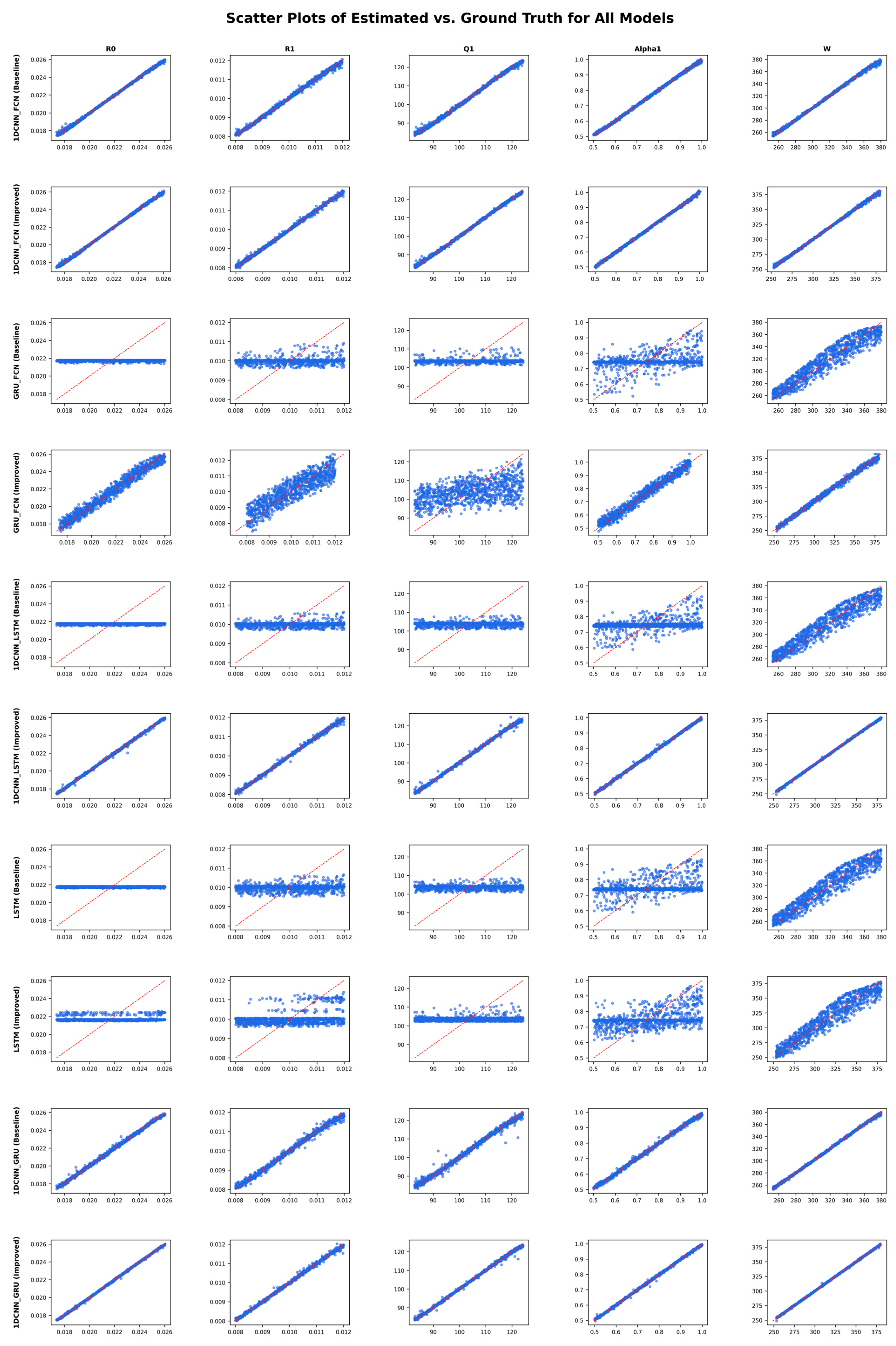
The core of the evaluation lies in the identification accuracy of the fundamental model parameters: the ohmic resistance (R₀), the charge transfer resistance (R₁), the constant phase element (Q₁), the fractional-order derivative (α), and the Warburg impedance element (W). Figure 6 presents a comprehensive visual assessment of the estimation accuracy for five distinct models, each with a baseline and an improved variant. The scatter plots, which correlate estimated values with their ground truth counterparts over 1,000 test samples, reveal several key insights. Ideal estimation would place all data points directly on the diagonal identity line, indicating a perfect match. Overall, the improved versions of the models demonstrate a clear enhancement in estimation accuracy, as evidenced by the tighter clustering of data points along the diagonal reference line. Among the five examined parameters (R₀, R₁, Q₁, α, and W), the resistive parameters R₀ and W are generally easier to identify, with all models exhibiting near-perfect linear correlations between predicted and true values for the improved versions—except for the LSTM model. For the capacitive parameter (Q₁) and the fractional order (α), larger deviations are observed, particularly in the baseline models, suggesting higher sensitivity to model architecture and data representation. The pure recurrent architectures (LSTM and GRU) show relatively greater dispersion in these parameters, indicating difficulties in capturing the nonlinear fractional-order dynamics solely through temporal dependencies. In contrast, models incorporating convolutional layers (1DCNN, 1DCNN + LSTM, and 1DCNN + GRU) achieve substantially improved alignment with the ground truth, demonstrating the advantage of spatiotemporal feature extraction. The improved versions of all hybrid models, especially 1DCNN + GRU, exhibit the most consistent performance across all parameters, with minimal bias and scatter. These results highlight that convolutional–recurrent fusion enhances parameter identifiability by leveraging both local feature extraction and temporal correlation learning. Additionally, R1 appears moderately difficult to estimate, though the improved hybrid models maintain high predictive fidelity. Overall, the results confirm that the proposed improvements effectively enhance robustness and accuracy in parameter estimation for fractional-order lithium-ion battery models.

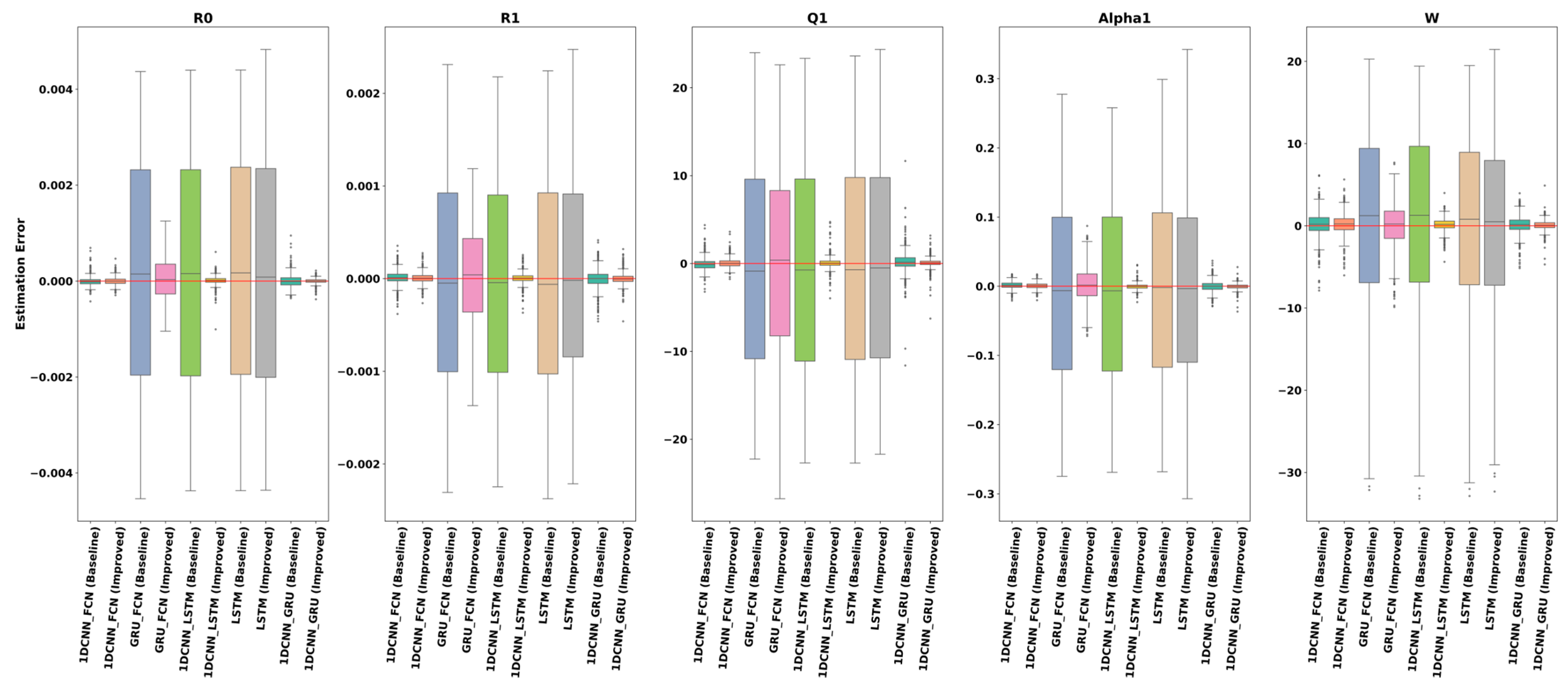
Figure 7 presents the estimation error distributions for all models across the five parameters, providing a quantitative complement to the scatter plots shown in Figure 6. Overall, the improved models consistently exhibit narrower interquartile ranges and smaller median deviations, confirming that the proposed enhancements effectively reduce estimation variance and bias. The 1DCNN-based hybrid models, particularly the 1DCNN + GRU (Improved) model, achieve the lowest error dispersion across all parameters, demonstrating superior robustness and generalization. Comparing architectures, the convolution–recurrent hybrids outperform both pure CNN and pure RNN models, highlighting the advantage of integrating local feature extraction with temporal modeling. These findings align with the scatter plot results, collectively confirming that the improved hybrid frameworks yield more accurate and stable parameter identification across all fractional-order components of the lithium-ion battery model. 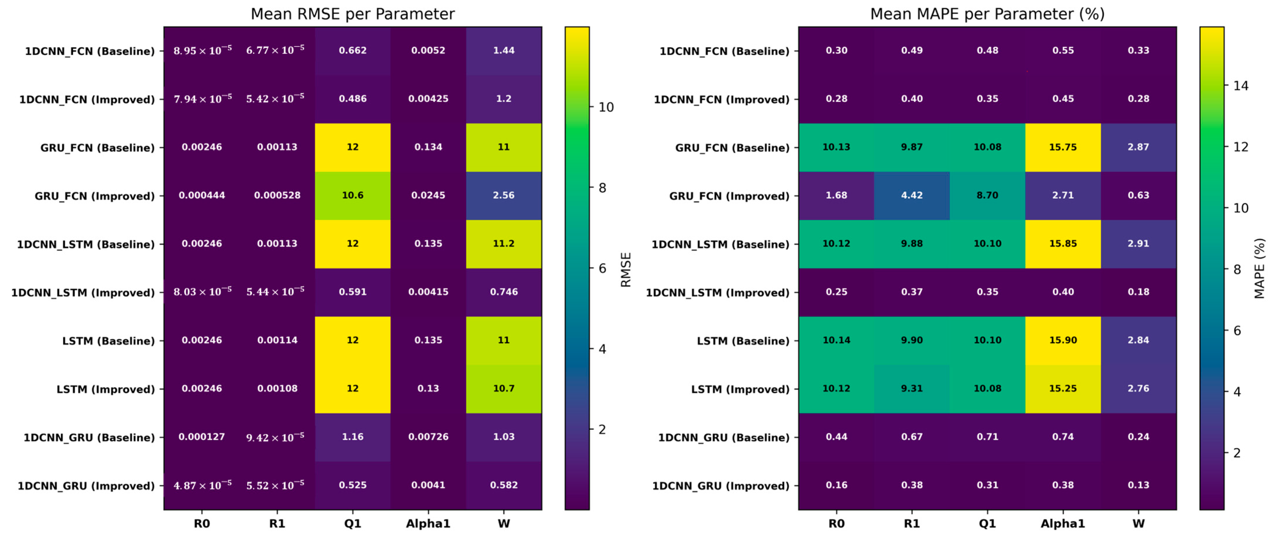Figure 8 presents heatmaps of the RMSE and MAPE, offering a definitive quantitative summary of model performance that strongly aligns with the preceding visual analyses from the scatter and box plots. The results provide unambiguous numerical evidence supporting the key conclusions about the efficacy of the model improvements, the performance ranking of the architectures, and the relative difficulty of parameter identification. The most prominent finding is the substantial performance gap between the baseline and improved models. The baseline variants are universally characterized by high error metrics, visualized as bright yellow and green hues, with MAPE often exceeding 9%. In stark contrast, the improved models consistently display dark purple and blue hues, representing dramatically lower errors. This confirms the overwhelming effectiveness of the proposed improvements in enhancing model accuracy and reliability. Furthermore, the heatmaps reaffirm the parameter identification hierarchy. For the majority of the improved models, the fractional-order exponent α₁ consistently yielded the highest MAPE values. This observation confirms that α is the most difficult parameter to identify with precision, while R₀ is identified with the highest fidelity.

The efficacy of the proposed FOM parameter identification methods was evaluated on a test set of 1000 samples, with the overall results summarized in

Table 3. Aggregated RMSE and MAPE for Parameter Estimation Across the 10 Model Variants.

Model	RMSE	MAPE (%)
1DCNN_FCN (Baseline)	0.42088	0.42993
1DCNN_FCN (Improved)	0.33886	0.35212
GRU_FCN (Baseline)	4.62582	9.73964
GRU_FCN (Improved)	2.63896	3.62933
1DCNN_LSTM (Baseline)	4.65831	9.77203
1DCNN_LSTM (Improved)	0.26827	0.31004
LSTM (Baseline)	4.61500	9.77574
LSTM (Improved)	4.56344	9.50254
1DCNN_GRU (Baseline)	0.43863	0.56150
1DCNN_GRU (Improved)	0.22232	0.27387

. For each of the ten model variants—baseline and improved versions of LSTM, GRU, 1DCNN-FCN, 1DCNN-LSTM, and 1DCNN-GRU—the overall RMSE and MAPE values were computed as the mean of the respective errors across all five model parameters. These numerical results establish a definitive performance hierarchy, reinforcing conclusions drawn from prior graphical analyses and quantifying the impact of the proposed improvements. The improved versions consistently outperformed their baseline counterparts, with hybrid architectures—particularly those incorporating 1D convolutional layers—forming the top tier of accuracy. A clear stratification emerged among the models, with 1DCNN_GRU, 1DCNN_LSTM, and standalone 1DCNN leading in performance. The 1DCNN_GRU (Improved) model was the top performer, achieving an RMSE of 0.2223 and a MAPE of 0.27%, representing nearly a 50% reduction in RMSE compared to its baseline version. Similarly, the 1DCNN_LSTM (Improved) variant exhibited dramatic improvement, reducing RMSE from 4.658 to 0.268 and MAPE from 9.77% to 0.31%, reflecting a performance increase of over 31-fold. This underscores a powerful synergistic effect between convolutional feature extraction and recurrent layers, enhanced by the improved framework. In contrast, standalone recurrent models lagged significantly. The improved GRU model recorded a MAPE of 3.63%, while the improved LSTM model had a high MAPE of 9.50%, showing only a marginal reduction from 9.77%. This minimal improvement suggests that the standalone LSTM architecture is fundamentally ill-suited for this task, as the enhanced techniques could not fully mitigate its inherent limitations. The magnitude of improvement from baseline to improved versions varied across models, with hybrid architectures exhibiting the most substantial gains. For instance, 1DCNN_FCN (Improved) showed solid progress, though it remained mid-tier among hybrids with a reduced RMSE. Meanwhile, GRU_FCN (Improved) halved its RMSE to 2.639 but still trailed the top performers. The standalone LSTM and GRU_FCN models exhibited more modest enhancements, with LSTM (Improved) reducing RMSE from 4.615 to 4.563, indicating limited responsiveness to the applied improvements. These results highlight the advantage of integrating convolutional layers with recurrent units, which effectively capture both spatial and temporal features critical for parameter estimation in this context. Ranking the models, 1DCNN_GRU (Improved) and 1DCNN_LSTM (Improved) led, followed by 1DCNN_FCN (Improved), with GRU_FCN (Improved) and LSTM (Improved) trailing significantly. The superior performance of hybrid models can be attributed to the complementary strengths of 1DCNN’s local feature extraction and the temporal modeling capabilities of LSTM or GRU, amplified by the proposed enhancements. The inclusion of Huber loss likely improved robustness to outliers, while SWA and EMA enhanced generalization, with their combined effect yielding the most substantial accuracy gains. This analysis affirms that the 1DCNN-GRU architecture, optimized with both techniques, provides the most accurate and robust solution for parameter identification in the FOM, as substantiated by the comprehensive metrics in Table 3.

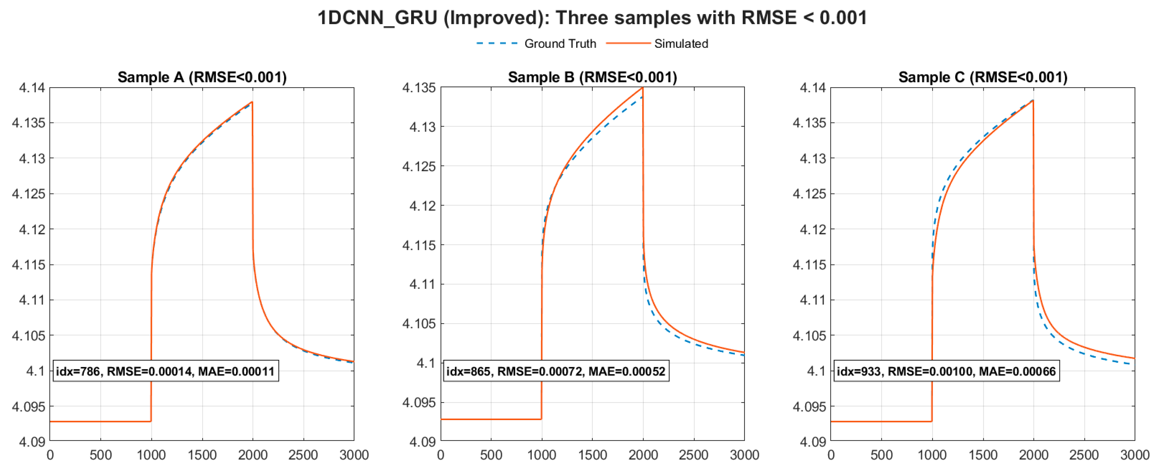
Accurate parameter estimation is essential; however, the ultimate validation of the identified model lies in its ability to precisely predict the battery’s terminal voltage. The parameters obtained from the test set were subsequently substituted into the realized FOM simulation platform to generate simulated voltage responses. The best-performing 1DCNN_GRU model achieves average RMSE and MAE values of 0.002059 and 0.001387, respectively, across 1000 test data points, further validating the accuracy of the proposed method. Figure 9 presents the simulated voltage responses alongside the ground truth for three randomly selected test samples. In every model and case, the simulated waveforms exhibit an exceptionally close overlap with the actual voltage profiles. This excellent visual agreement, quantitatively supported by consistently low RMSE and MAE values displayed on each plot, confirms that all improved models effectively leverage their estimated parameters to accurately reconstruct the battery’s dynamic behavior with high fidelity.

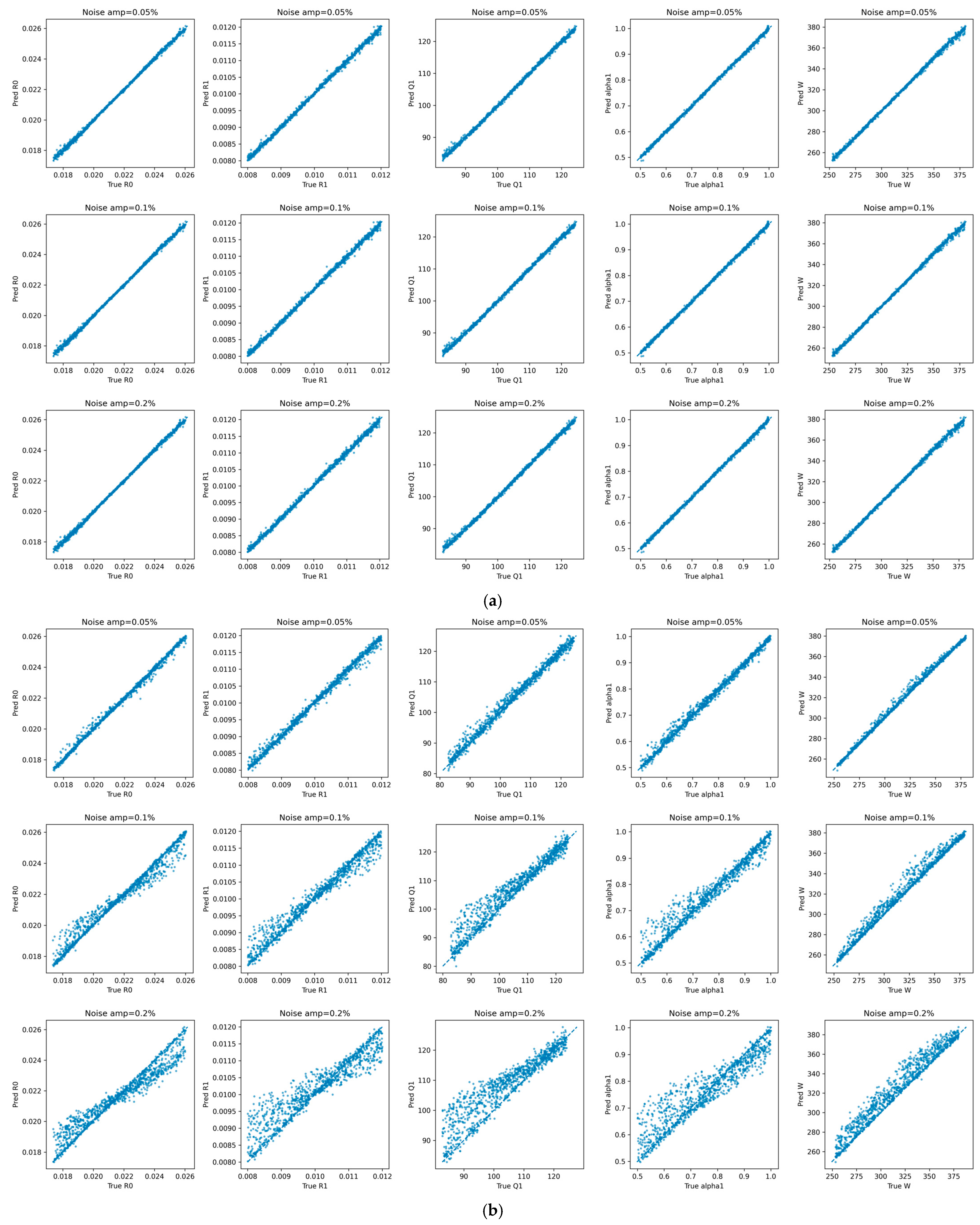
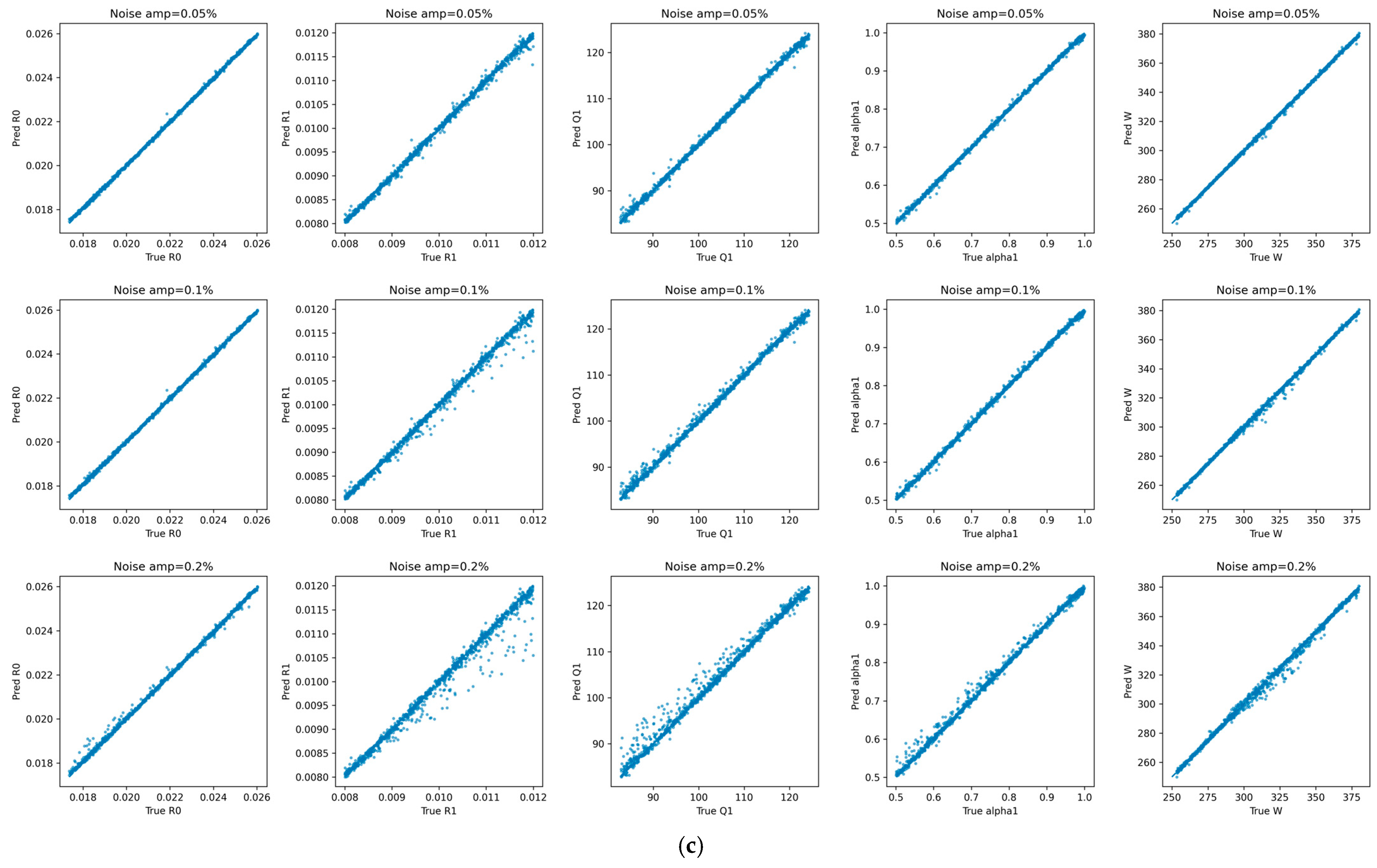
To simulate real-world measurement conditions, synthetic voltage waveforms were corrupted with noise to assess the robustness of the proposed deep learning methods. Considering that the voltage measurement accuracy of typical commercial battery cyclers is generally lower than 0.1% full scale, three noise levels0.05%, 0.1%, and 0.2% of the signal amplitude—were tested, representing optimistic, typical, and worst-case scenarios, respectively.

Table 4. Performance Of The 3 Best Performing Models Under Different Levels of Noise.

Model	Noise Level	RMSE	MAPE (%)
1DCNN_FCN (Improved)	0.05%	0.33889	0.35359
RMSE (noise = 0): 0.33886	0.1%	0.34105	0.35675
MAPE (noise = 0): 0.35212	0.2%	0.35482	0.36861
1DCNN_LSTM (Improved)	0.05%	0.73823	0.75877
RMSE (noise = 0): 0.26827	0.1%	1.89417	1.90011
MAPE (noise = 0): 0.31004	0.2%	3.45218	3.72231
1DCNN_GRU (Improved)	0.05%	0.25453	0.30438
RMSE (noise = 0): 0.22232	0.1%	0.38005	0.37900
MAPE (noise = 0): 0.27387	0.2%	0.72605	0.63324

presents the RMSE and MAPE of the three top-performing models under these noise conditions, while Figure 10 shows the scatter plots of the parameter identification results across varying noise intensities. Based on the results presented in Table 4 and Figure 10, the robustness of the three improved models against simulated measurement noise was evaluated. The 1DCNN_GRU (Improved) model demonstrates superior noise immunity, maintaining relatively stable RMSE and MAPE values even at a 0.2% noise level (RMSE: 0.726, MAPE: 0.633%). Its performance degradation is the most gradual among the three, indicating a strong ability to learn robust features from noisy inputs. In contrast, the 1DCNN_LSTM (Improved) model exhibits significant sensitivity to noise. While its performance is excellent with clean data, its RMSE and MAPE deteriorate dramatically with increasing noise, surging to 3.452 and 3.722%, respectively, at the 0.2% noise level, which suggests potential overfitting to the clean training data or instability in its temporal processing under perturbation. The 1DCNN_FCN (Improved) model shows moderate and consistent robustness. Its error metrics increase only slightly across the tested noise levels, reflecting a stable architecture less affected by minor input variations. This analysis confirms that the 1DCNN_GRU model possesses the most reliable anti-interference capability, making it the most suitable candidate for deployment in real-world scenarios where sensor data is often contaminated with noise. The varying degrees of robustness highlight the critical impact of the recurrent layer’s architecture on model stability.

5. Conclusions

This study demonstrates the effectiveness of a hybrid deep learning framework for identifying parameters in fractional-order models of lithium-ion batteries, addressing limitations in accuracy and adaptability. By integrating convolutional and recurrent neural network layers, the proposed approach enhances feature extraction and captures temporal dependencies, pioneering the application of deep learning to fractional-order model parameter identification. A simulation platform was employed to generate diverse datasets, while the Optuna framework was utilized for hyperparameter optimization. To improve robustness, techniques such as Huber loss, stochastic weight averaging, and exponential moving averaging were incorporated to mitigate the effects of outliers and ensure stable convergence. The contributions are supported by quantitative results on a 1,000-sample test set. The improved 1DCNN–GRU model achieved an overall RMSE of 0.2223 and MAPE of 0.27%, outperforming baseline models by up to 50% in RMSE (e.g., reduced from 0.4386) and surpassing other hybrid models such as 1DCNN–LSTM (MAPE 0.31%). In contrast, standalone recurrent models, including the improved LSTM, exhibited significantly higher errors, with a MAPE of 9.50%. Scatter plots confirmed low estimation bias for the fractional-order coefficient α, while box plots indicated narrower interquartile ranges across parameters. Heatmaps further illustrated the hierarchy of estimation difficulty, identifying α as the most challenging parameter—yet it was estimated with a MAPE below 1% in the top-performing models. Resistive components (R₀, W) were predicted with near-ideal accuracy, while parameters Q₁ and R₁ showed reduced variance. Terminal voltage reconstruction achieved an average RMSE of 0.002059 and MAE of 0.001387, confirming close alignment with the reference waveform and underscoring the practical reliability of the proposed method. This work establishes hybrid deep learning as a pivotal advancement in electrochemical modeling, successfully balancing high precision with computational efficiency.

Although noise has been deliberately introduced into synthetic voltage waveforms to approximate real-world conditions, the robustness of the proposed models under such perturbations varies significantly. While the 1DCNN_GRU model demonstrates exceptional noise immunity with minimal performance degradation, the 1DCNN_LSTM model exhibits considerable sensitivity, with error metrics increasing sharply at higher noise levels. This indicates that while some architectures show satisfactory resilience, others may be less reliable. Furthermore, using actual measured waveforms as inputs presents challenges beyond synthetic noise, including sensor drift, environmental interference, and non-stationary disturbances, which are likely to pose greater difficulties. Future work will therefore focus on in-depth investigations in this area to further bridge the gap between simulated tests and real-world deployment, with a specific emphasis on enhancing model generalization against a broader spectrum of real-world imperfections.