Article

A Hybrid CNN–LSTM–Attention Mechanism Model for Anomaly Detection in Lithium-Ion Batteries of Electric Bicycles

1
High-Tech Standardization Research Institute, China National Institute of Standardization, Beijing 100191, China
2
School of Management and E-Business, Zhejiang Gongshang University, Hangzhou 310018, China
*
Author to whom correspondence should be addressed.
Batteries 2025, 11(10), 384; https://doi.org/10.3390/batteries11100384
Submission received: 31 August 2025 / Revised: 16 October 2025 / Accepted: 17 October 2025 / Published: 20 October 2025
(This article belongs to the Special Issue State-of-Health Estimation of Batteries)

Abstract

To improve the accuracy and stability of anomaly detection in lithium-ion batteries for electric bicycles, in this study, we propose a hybrid deep learning model that integrates a convolutional neural network (CNN), long short-term memory (LSTM) network, and attention mechanism to extract local temporal features, capture long-term dependencies, and adaptively focus on key time segments around anomaly occurrences, respectively, thereby achieving a balance between local and global feature modeling. In terms of data preprocessing, separate feature sets are constructed for charging and discharging conditions, and sliding windows combined with min–max normalization are applied to generate model inputs. The model was trained and validated on large-scale real-world battery operation data. The experimental results demonstrate that the proposed method achieves high detection accuracy and robustness in terms of reconstruction error distribution, alarm rate stability, and Top-K anomaly consistency. The method can effectively identify various types of abnormal operating conditions in unlabeled datasets based on unsupervised learning. This study provides a transferable deep learning solution for enhancing the safety monitoring of electric bicycle batteries.

1. Introduction

In recent years, electric bicycles have become an important means of short-distance transportation for urban residents in China due to their environmental friendliness, convenience, and affordability. According to the China Bicycle Association, the number of electric bicycles nationwide has exceeded 300 million, with annual sales consistently above 30 million units. However, lithium-ion batteries, which are the core power component of electric bicycles, are susceptible to various potential anomalies during operation, such as overcharging, overdischarging, overheating, cell voltage imbalance, and internal short circuits [1,2,3,4,5]. These anomalies not only shorten the cycle life of batteries but may also lead to serious safety incidents. Consequently, anomaly detection in battery operating states has become one of the key technologies for ensuring the safe operation of electric bicycles. Existing techniques can be broadly categorized into three groups: rule-based and statistical analysis methods [6], traditional machine learning methods [7], and deep learning-based time-series modeling approaches [8].
Early approaches to battery anomaly detection primarily relied on manual experience and statistical features. For example, threshold ranges for key parameters, such as voltage, current, and temperature were predefined, and anomalies were identified by monitoring whether real-time values exceeded these limits. These methods are simple to implement, computationally efficient, and suitable for resource-constrained embedded systems [9]. However, due to their limited capability in modeling temporal correlations among features and the fact that static thresholds are usually derived from laboratory test data, they struggle to adapt to individual battery differences and varying operating environments. As a result, these methods are prone to false alarms and missed detections under complex working conditions [10].
With the advancement of data acquisition and storage technologies, researchers have begun adopting machine learning methods such as support vector machines, decision trees, random forests, Isolation Forests, and One-Class SVMs for battery anomaly detection. These approaches typically require the construction of fixed-length feature vectors, which are then input into classifiers for training and prediction [11]. Compared to rule-based methods, machine learning techniques can exploit correlations among multidimensional features, thus improve detection accuracy [12]. However, they heavily rely on feature engineering, struggle to capture nonlinear temporal dependencies, and exhibit limited adaptability to changes in data distribution.
In recent years, deep learning has demonstrated significant advantages in handling complex time-series data that are high-dimensional and long in sequence [13]. CNNs are capable of extract temporal patterns within local windows, making them suitable for capturing short-term feature variations. LSTM networks excel at preserving long-term dependencies and are thus effective for modeling the slow-changing characteristics of battery states [14]. Attention mechanisms learn weight distributions across time steps and adaptively focus on critical temporal segments, achieving outstanding performance in natural language processing and time-series forecasting. Moreover, in multivariate time-series anomaly detection scenarios, models that combine CNN–LSTM architectures with attention mechanisms have proven to achieve superior performance [15].
At present, hybrid models that combine CNNs and LSTM have been effectively validated across multiple domains. Kaushik [16] employed these architectures in speech emotion recognition, where CNNs were used for local feature extraction and LSTM for capturing long-term dependencies, achieving high accuracy. Regarding industrial equipment fault prediction and remaining useful life estimation tasks, the studies of Borré et al. [17] and Wahid et al. [18] also confirmed the significant advantages of these models in handling equipment vibration and sensor data. Gamaleldin et al. [19] applied a hybrid CNN–LSTM framework in insurance risk assessment, enhancing the recognition of claim trends and the effectiveness of risk classification.
Several studies have further incorporated self-attention mechanisms to improve model interpretability and detection accuracy. Jiang et al. [20] combined convolutional autoencoders with self-attention to achieve automated SOH (State of Health) feature extraction; Ouyang et al. [21] utilized multi-head self-attention to enhance SOH prediction; Shi et al. [22] optimized SOC (State of Charge) curve estimation through a spatiotemporal self-attention Transformer network; and Hussein et al. [23] highlighted the performance improvements brought by attention mechanisms in Transformers through the assignment of importance weights in SOC estimation.
In summary, although significant progress has been made in battery state estimation and health prediction, the field of unsupervised anomaly detection for real-world e-bike batteries remains relatively underexplored. Existing studies have often relied on small-scale laboratory datasets or focused on SOH and SOC estimation, limiting their applicability to complex, unlabeled operational data collected under diverse environmental and usage conditions. To address these challenges, this study develops a hybrid deep learning framework that integrates CNNs, LSTM networks, and an attention mechanism. The proposed model leverages CNNs to extract local temporal fluctuations, LSTMs to capture long-term dependencies, and the attention mechanism to adaptively emphasize critical time segments related to anomalies. Furthermore, by adopting a reconstruction-based unsupervised learning strategy and introducing a Top-K Jaccard similarity evaluation, the framework ensures stable and interpretable anomaly detection across multiple batteries and operating conditions. This work thus contributes a scalable and data-driven solution for intelligent battery safety monitoring, bridging the gap between theoretical modeling and real-world deployment.

2. Materials and Methods

2.1. CNN–LSTM–Attention Model

CNNs are deep learning models characterized by local receptive fields and weight sharing, which enable them to effectively extract local patterns and spatial features from input signals [24]. In this study, CNN performs one-dimensional convolution operations on time series constructed using a sliding window, in order to capture variation trends between adjacent time steps. For an input sequence X T × d , where T denotes the window length and d represents the feature dimension, the convolutional layer is computed as follows:
h t c = σ k = 0 K 1 W k X t + k + b
where K denotes the kernel size, W k represents the kernel weight, b is the bias term, and σ is a nonlinear activation function (e.g., ReLU). Through convolution operations, the model can identify short-term feature patterns such as sudden voltage fluctuations and abnormal temperature rises, thereby providing high-quality feature inputs for subsequent temporal modeling.
LSTM networks were first proposed by Hochreiter and Schmidhuber in 1997, introducing the structures of input, forget, and output gates, which effectively address the gradient vanishing problem of traditional recurrent neural networks (RNNs) [25]. Greff et al. systematically analyzed various LSTM variants and the role of gating mechanisms in mitigating gradient vanishing [26]. The update equations of an LSTM cell are given as follows:
f t = σ W f h t 1 , x t + b f i t = σ W i h t 1 , x t + b i C ˜ t = tan h W C h t 1 , x t + b C C t = f t C t 1 + i t C ˜ t o t = σ W o h t 1 , x t + b o h t = o t tan h C t
where σ denotes the sigmoid activation function, represents the Hadamard product, and h t is the hidden state in the time step t . In this study, LSTM is primarily employed to capture long-span variation patterns in battery operating parameters.
Attention mechanisms assign different importance weights to different time steps and features, enabling models to focus on more critical temporal positions. In this study, the hidden state h t in each time step output by the LSTM is passed through the attention layer to compute its corresponding weight, α t , yielding the weighted feature representation:
α t = exp u t w a k = 1 T exp u k w a
z = t = 1 T α t h t
where u t = tan h W a h t + b a and W a denote the attention weight vectors, and z represents the weighted sequence representation. Through the attention mechanism, the model can highlight the feature contributions of time steps surrounding anomalies, such as critical signal fluctuations occurring prior to short circuits and abnormal temperature rises.
CNNs can extract local patterns from time-series data through one-dimensional convolutions, such as short-term voltage fluctuations and instantaneous temperature variations. LSTM is suitable for capturing long-term dependencies, such as voltage decay trends over charge–discharge cycles. Attention mechanisms assign different weights to each time step according to its importance in the input sequence, thereby automatically focusing on critical moments around anomaly occurrences during the detection process. By combining a CNN, LSTM, and an attention mechanism, our model is able to simultaneously capture both local and global temporal features, improving the accuracy and robustness of anomaly detection.
In this study, we propose a CNN–LSTM–Attention-based model that integrates the advantages of all three components for anomaly detection in lithium-ion batteries of electric bicycles. The workflow of the proposed model is illustrated in Figure 1.
Compared with sequence modeling approaches that solely rely on LSTM or GRUs, the CNN–LSTM–Attention architecture can more effectively capture both local fluctuations and global dependencies [27]. Specifically, a CNN is employed to extract local temporal features within sliding windows, LSTM is used to capture long-term dependencies across sequences, and the attention mechanism further assigns feature weights based on the outputs of the LSTM.
  • Feature Extraction and Temporal Modeling
The input battery monitoring data are denoted as X T × d , where T is the time window length and d is the feature dimension. First, the CNN performs one-dimensional convolution on X , producing a local feature map, H c , which is used to capture short-term parameter fluctuation patterns such as sudden changes in temperature and voltage. Subsequently, the convolutional output is fed into the LSTM to generate a sequence of hidden states, { h 1 , h 2 , h 3 , , h T } , which characterize long-term dependencies across the time span.
2.
Attention Weighting
To enable the model to focus on time segments that contribute more to anomaly identification, an attention mechanism is introduced to compute an importance weight, α t , for each time step. By performing a weighted summation, a feature vector, z , is obtained, which integrates both global dependencies and information from critical moments.
3.
Reconstruction and Error Calculation
The weighted feature vector z is fed into a fully connected layer to output the reconstructed values of multiple parameters, x ^ t d . During the training phase, the model aims to minimize the reconstruction error, with the mean squared error (MSE) adopted as the loss function:
L = 1 d j = 1 d x t , j x ^ t , j 2
In the context of battery anomaly detection, the CNN performs one-dimensional convolutions on multivariate features within each time window, efficiently capturing abrupt patterns of voltage, temperature, and current variations on short time scales, while reducing redundancy in the raw input sequences and alleviating computational burdens. Building on the convolutional outputs, the LSTM establishes dynamic dependencies across time steps to characterize the long-term evolution of battery states, thereby enhancing the detection of slowly developing anomalies. The introduced attention mechanism enables the model to focus on time segments and feature dimensions that contribute most to anomaly identification, mitigating information loss caused by gradient attenuation in long-sequence modeling and significantly improving responsiveness to local sudden anomalies. In addition to improving anomaly detection performance, the attention weights can be extracted and visualized. This enables us to interpret which temporal segments the model focuses on, thereby enhancing the transparency and explainability of the anomaly detection process. Overall, this architecture not only outperforms single-sequence models in terms of accuracy but also demonstrates stronger robustness and generalization ability when handling multi-scale features, complex fluctuation patterns, and long-term dependencies.

2.2. Research Dataset

The dataset used in this study was obtained from real-time monitoring data on lithium-ion batteries in electric bicycles during actual operation, and it did not contain labels indicating normal or abnormal states. The data collection period covered battery states under various environmental temperatures and different charging and discharging conditions, thereby providing a comprehensive reflection of performance variations and anomaly characteristics. The raw dataset contained operational records from 10 batteries, comprising approximately 4 million data points in total. Each record included a Unix timestamp and multiple parameters related to battery operation.
To ensure independence between model training and validation, the data from the 10 batteries were partitioned into training, validation, and test sets. Specifically, the data from 7 batteries (2,433,005 records) were used for training, with 80% and 20% further allocated to the training and validation subsets, respectively, while the remaining 3 batteries were reserved for testing. According to the operating state of the batteries, the dataset was categorized into two feature types: discharging and charging. The selected parameter dimensions and their corresponding descriptions are summarized in Table 1. Most of the parameter descriptions are generated based on technical or industry standards like IEC 62660-1 [28], IEC 62660-2 [29], GB/T 36972-2018 [30], etc.
In the data preprocessing stage, missing values were first handled, and outliers were removed. Then, time-series samples were generated using a sliding window approach, with the window length set to 30 s and the step size set to 1 s. Subsequently, min–max normalization was applied to the features to eliminate the influence of dimensional differences. To ensure training stability, separate datasets were constructed for discharging and charging features, and corresponding CNN–LSTM–Attention models were trained independently in the subsequent experiments for anomaly detection under different operating conditions.
In this study, feature selection was primarily based on domain knowledge of battery operating parameters, and the time-series data were processed using a sliding window approach combined with min–max normalization to remove the influence of dimensional differences. This design ensured that both short-term fluctuations (captured within each window) and long-term dependencies (modeled by LSTM units) could be effectively learned.
We are aware that more advanced feature selection and attribution techniques, such as mutual information, recursive feature elimination (RFE), and SHAP values, have been proposed to capture nonlinear dependencies between features and enhance interpretability. However, considering that the dataset used in this work was high-frequency and unlabeled, the primary objective was to retain as much raw operational information as possible for unsupervised anomaly detection. Therefore, we deliberately avoided aggressive feature elimination to prevent the loss of potentially anomaly relevant signals.

2.3. Environment Setup

All training and detection experiments were conducted on a desktop computer (Hangzhou, Zhejiang, China)in a Windows 11 environment, which equipped with a CPU (Intel Core i5-12600KF), a GPU (NVIDIA RTX 4060Ti 8 GB), and 32 GB of RAM. The deep learning framework used was PyTorch 2.5.0 with CUDA 12.4 and cuDNN 9.1.0.
In the proposed CNN–LSTM–Attention model, the convolutional module adopts a one-dimensional convolution structure, with 8 input channels, 64 output channels, a kernel size of 3 × 1, and a stride of 1. A ReLU activation function is used to extract local temporal features. The convolutional layer is followed by a one-dimensional max-pooling layer (MaxPooling1d) with a pooling window size of 2 and a stride of 2, which reduces the feature dimensionality while retaining the most salient information.
The LSTM module consists of a single-layer, unidirectional structure with an input dimension of 64 and 64 hidden units, enabling the capture of long-term temporal dependencies. Its output sequence is further processed by a self-attention mechanism layer to obtain feature representations that are more focused on critical time segments.
The fully connected part includes two dense layers. The first layer flattens the attention output and maps it to a 32-dimensional hidden layer with ReLU activation. The second layer maps it to a dimension equal to the number of input features, thereby reconstructing the multivariate feature values of each time window. Finally, the output layer is linear and produces the reconstructed values of each feature, which are then used for subsequent reconstruction error computation and anomaly detection.
During training, the Adam optimizer was employed for parameter updates, with Automatic Mixed Precision (AMP) training enabled. The learning rate was set to 0.0001, with the first-order momentum decay coefficient β 1 = 0.9 and the second-order momentum decay coefficient β 2 = 0.999 . The mean squared error (MSE Loss) was used as the loss function to measure the discrepancy between the input and the reconstructed output. The batch size was set to 256, and the number of training epochs was fixed at 20. Early stopping was not applied to ensure sufficient convergence of the model.
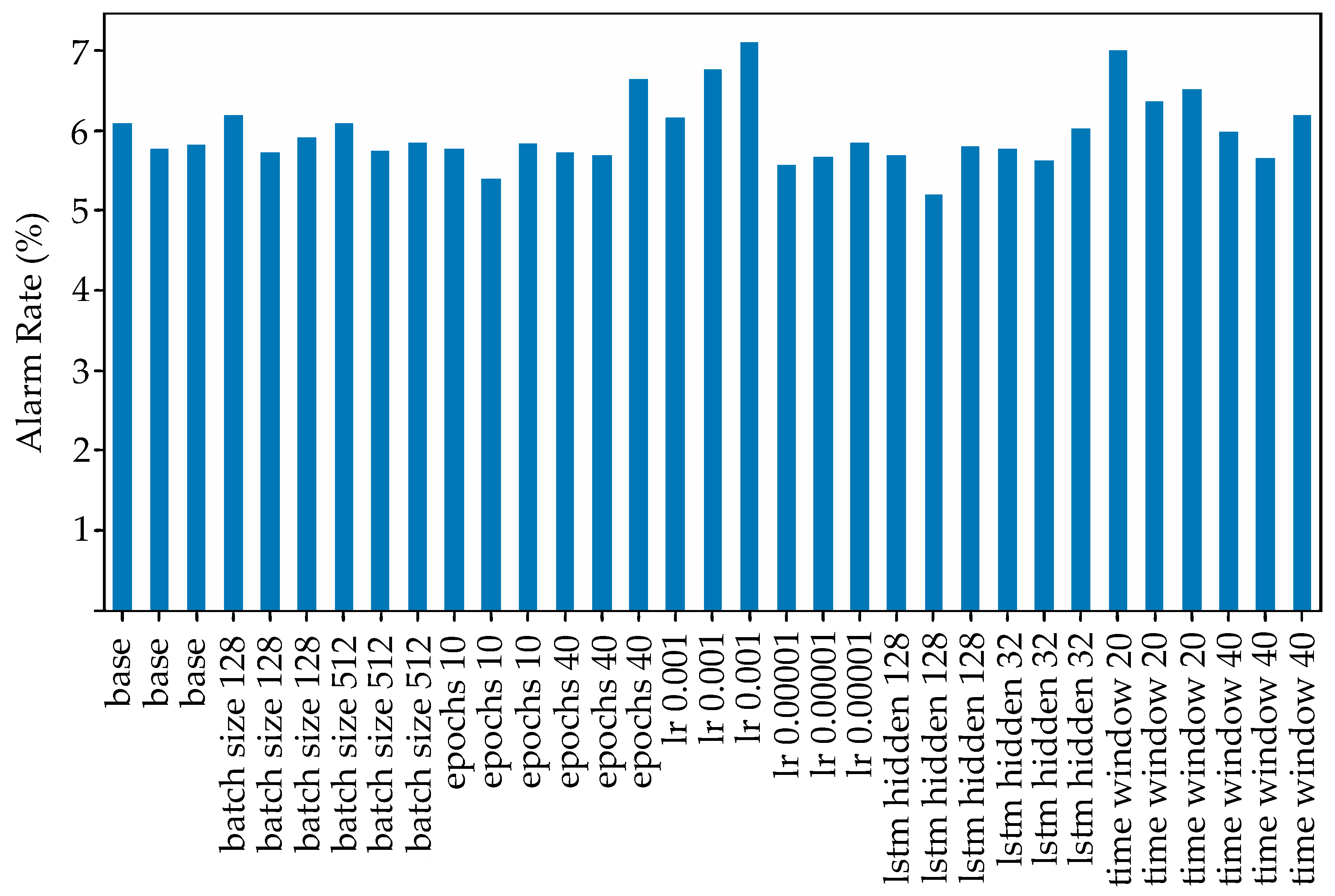
To evaluate the robustness of the proposed model under different parameter configurations, we conducted a sensitivity analysis using the One-at-a-Time method. Based on the baseline settings described previously, five key hyperparameters were examined: batch size, the number of training epochs, the learning rate, the number of LSTM hidden units, and time window length. In each experiment, only one hyperparameter was varied while the others were kept fixed, and the results were compared against those of the baseline configuration.
As shown in Figure 2, the average alarm rate under different hyperparameter configurations remained within the 5–7% range, with only minor fluctuations. This indicates that the model’s detection performance was not highly sensitive to hyperparameter perturbations. Figure 3 presents the outcomes of the stability comparison, where the consistency of detection results across different experiments was evaluated using the Jaccard index at the Top 1% and Top 5% levels. The results demonstrate that the adopted configuration consistently achieved the highest or near-highest average values across both metrics, while also exhibiting the smallest standard deviation. This suggests that the model maintained strong consistency and robustness under different random seeds. These findings further validate the rationality of the baseline parameter settings. Overall, the adopted configuration achieves a favorable balance between detection accuracy and stability; regardless of hyperparameter perturbations or threshold adjustments, both the overall alarm level and the consistency of detection results remain stable, confirming that the chosen hyperparameter settings are both reasonable and robust.

2.4. Model Training and Data Detection

Model training first requires generating training samples from the cleaned and normalized training dataset using a fixed time window. These samples are then fed into the constructed CNN–LSTM–Attention network, which is iteratively optimized on the training set according to specified hyperparameters, such as batch size, learning rate, and the number of epochs, until the model achieves the desired performance on the test set. The trained model weights and normalization parameters are subsequently saved for later detection.
Before the test set data are input into the model, they must undergo the same preprocessing steps as those in the training stage, including handling missing values and outliers, aligning feature order, applying normalization (using the parameter files saved from training), and performing sliding window segmentation.
In the detection phase, the model adopts a reconstruction-based anomaly detection strategy rather than conventional time-series forecasting. Similar anomaly detection strategies have been adopted in recent works; for instance, a hybrid autoencoder–ResNet framework was applied for anomaly filtering to improve remaining useful life (RUL) prediction in lithium-ion batteries [31]. Specifically, given an input time window, X t : t + T 1 , of the length T (with T = 30 ), the model reconstructs the expected normal feature values, X ^ t : t + T 1 , of the same window based on the normal operating patterns learned during training. Instead of predicting future data beyond the window, this approach performs a “denoising” normalization of the current input window itself. The anomaly score is then obtained by comparing the actual values with their reconstructed counterparts, measured as the mean reconstruction error:
e = 1 T F i = 1 T j = 1 F X i , j X ^ i , j
where F denotes the feature dimension, X i , j is the actual value of the feature j in the time step i within the window, and X ^ i , j is the corresponding reconstructed value.
Since the dataset used in this study does not contain manual labels, it is not feasible to directly build a classification model through supervised learning; therefore, unsupervised methods must be employed for anomaly detection [32,33]. Accordingly, a threshold needs to be defined based on the statistical distribution. In this work, the 95th percentile of the reconstruction error distribution from the training set is adopted as the decision threshold. Such a tail quantile-based threshold setting relies on the residual distribution of the training set, thus providing a statistical basis [34]. In unsupervised anomaly detection, this approach balances sensitivity and specificity, thereby reducing excessive false positives and false negatives [35]. As the dataset is derived from monitoring data of electric bicycles during real-world operation, it is reasonable to assume that the vast majority of samples represent normal states, which satisfies the fundamental assumption of the reconstruction-based anomaly detection strategy.
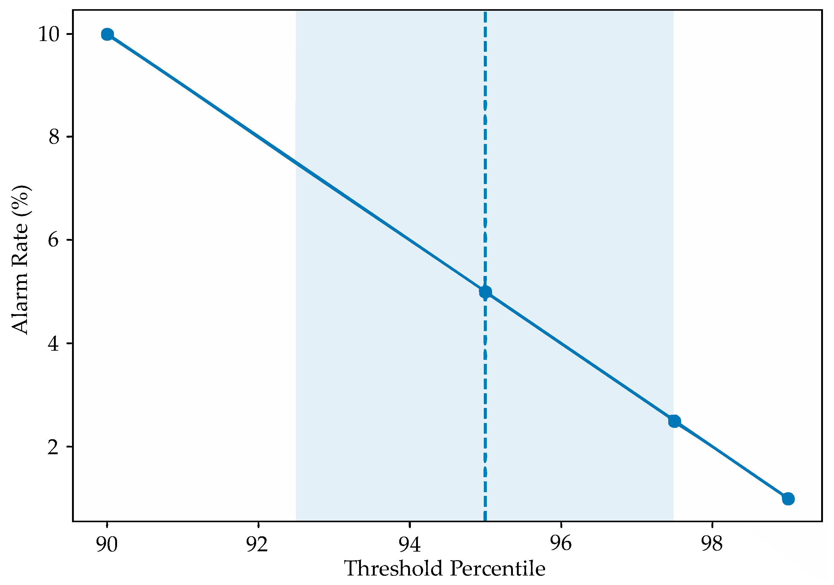
In unsupervised anomaly detection, threshold selection plays a critical role. Common strategies include fixed quantiles, statistical tests, and false alarm rate control. In this study, we examined multiple quantile thresholds (90%, 95%, 97.5%, and 99%) to analyze how the alarm rate varied with threshold settings (Figure 4). The results show a monotonic decrease in the alarm rate as the threshold increased, with the curve exhibiting smooth behavior and no abnormal fluctuations. The 95% quantile was chosen as the baseline threshold, as it lies in the middle of the curve: it avoids excessive alarms caused by overly low thresholds while preventing missed detections associated with overly high thresholds. This choice reflects a well-balanced and robust setting.
When the mean reconstruction error e exceeds a predefined threshold, θ , the corresponding time window is identified as containing an anomaly. This detection approach does not require prior knowledge of future data, enabling anomaly identification based solely on the current operating state. By using the normal patterns learned by the model as a baseline, this method can effectively detect various types of anomalies, including sudden changes, drifts, and long-term distortions.

3. Results

In this section, we comprehensively evaluate the proposed CNN–LSTM–Attention model and compare its performance against both classical anomaly detection methods and recent advanced deep models.
  • Isolation Forest (IF): A tree-based ensemble method that recursively partitions the feature space to isolate anomalous points.
  • One-Class Support Vector Machine (OCSVM): A kernel-based model that learns the boundary of normal samples and identifies points outside the boundary as anomalies.
  • Autoencoder (AE): A typical deep learning tool based on reconstruction error, employing a symmetric encoder–decoder architecture with the objective of minimizing reconstruction loss.
  • Anomaly Detection Transformer with Convolution (ADTC-Transformer): A recently proposed anomaly detection framework based on Transformer structures, which leverages temporal self-attention to enhance feature interactions and improve detection stability.
  • Attention Mechanism–Multi-scale Feature Fusion (AM-MFF): An attention-based multi-scale feature fusion model that combines convolutional and recurrent components with feature fusion mechanisms to capture complex temporal dependencies in battery data.
For fairness, all three baseline methods were implemented using the same feature set, sliding window strategy, and normalization procedure.

3.1. Training Phase

3.1.1. Convergence Analysis

Convergence analysis was conducted by recording the average training loss and validation loss in each epoch during the training process. This was used to evaluate whether the model could achieve stable convergence and to examine the presence of overfitting or underfitting. Comparing the trends of the two curves, if both exhibit a decreasing pattern without significant divergence, this indicates that the model performed consistently on both the training and validation datasets, thereby demonstrating good convergence.
Figure 5 illustrates the variation in average reconstruction loss on the training and validation sets over 20 epochs. It can be observed that both curves decrease rapidly within the first five epochs and then gradually level off. Moreover, the training and validation curves remain closely aligned without noticeable divergence, indicating that the model did not suffer from overfitting on this dataset.

3.1.2. Generalization Verification

Generalization evaluation was conducted to assess the stability of the model’s performance on unseen data, i.e., its generalization ability. The method involved comparing the reconstruction error distributions of the training set and the validation set by calculating the Kolmogorov–Smirnov (KS) statistic and the Wasserstein distance. The KS statistic measures the maximum difference between two cumulative distribution functions, where values closer to 0 indicate higher similarity [36]. The Wasserstein distance quantifies the minimum cost required to transform one distribution into another, with smaller values likewise indicating greater similarity [37].
To evaluate the generalization ability of the proposed CNN–LSTM–Attention model, we compared the distribution of reconstruction errors between training and validation sets using the two above-mentioned metrics. As shown in Table 2, the error distributions of the training and validation sets largely overlap for both charging and discharging data, with KS values around 0.10 and Wasserstein distances close to zero. These results indicate that the model achieved consistent reconstruction performance across different datasets, demonstrating good generalization ability.
For a broader comparison, Table 3 reports the same metrics for both classical anomaly detection methods (AE, IF, OCSVM) and two recently proposed advanced deep models (ADTC-Transformer and AM-MFF). The classical methods exhibit the lowest KS and Wasserstein values, but this is mainly due to their limited model complexity, which results in underfitting and overly simplistic decision boundaries. Although such models appear highly consistent between training and validation sets, their ability to capture complex anomaly patterns is severely constrained.
By contrast, the advanced models, ADTC-Transformer and AM-MFF, show noticeably higher KS and Wasserstein values than those of our proposed method, reflecting larger discrepancies between training and validation sets. This suggests that while these models attempt to capture more complex dependencies, their stability across data partitions is weaker.
Overall, the proposed CNN–LSTM–Attention model achieves a favorable balance. Its KS and Wasserstein values remain small and comparable to those of classical methods, while it still benefits from richer temporal and multi-scale feature extraction. This balance enables the model to maintain robust generalization across unseen data, without suffering from the instability of advanced baselines or the underfitting of classical methods.

3.2. Detection Phase

In the detection phase, the decision rule established during model training was applied, namely using the 95th percentile of the reconstruction error distribution from the training set as the threshold. When the average reconstruction error of a test sample exceeded this threshold, the corresponding time window was identified as anomalous. The three batteries used for evaluation were numbered 342421544, 342425605, and 342429831, and their detection results are assessed as follows.

3.2.1. Threshold and Alarm Rate Stability

Under the same threshold criterion, the overall alarm rates of the three batteries were all close to 5%. Moreover, the proportions of alarms for both discharging and charging feature types were consistent with the expectations derived from the training set, as shown in Table 4. This indicates that the threshold exhibited good transferability across different detection targets, and the model demonstrated favorable performance in terms of distribution stability.
To further examine robustness, the proposed CNN–LSTM–Attention model was benchmarked against three classical anomaly detection frameworks, namely autoencoder, Isolation Forest, and One-Class SVM, as well as two recent advanced deep learning architectures, ADTC-Transformer and AM-MFF. The detailed results are presented in Table 5.
The results show that One-Class SVM produced the lowest average alarm rate across all batteries. However, its performance fluctuated considerably, with excessively high alarm rates observed in specific cases, such as the discharging condition of battery 342429831. This instability reflects the method’s limited adaptability to nonlinear and high-dimensional data. Isolation Forest and autoencoder recorded slightly higher average alarm rates and were prone to generating false alarms in certain scenarios, indicating insufficient cross-battery robustness.
The advanced models, ADTC-Transformer and AM-MFF, achieved higher overall averages, exceeding six percent, which suggests that their capacity to capture complex temporal dependencies comes at the cost of stability under real-world variability. By contrast, the proposed CNN–LSTM–Attention model consistently maintained alarm rates close to five percent across all batteries and operating conditions. This balance between sensitivity and stability highlights its ability to achieve reliable cross-battery generalization and underscores its suitability for deployment in practical safety monitoring systems.

3.2.2. Distribution of Anomaly Scores

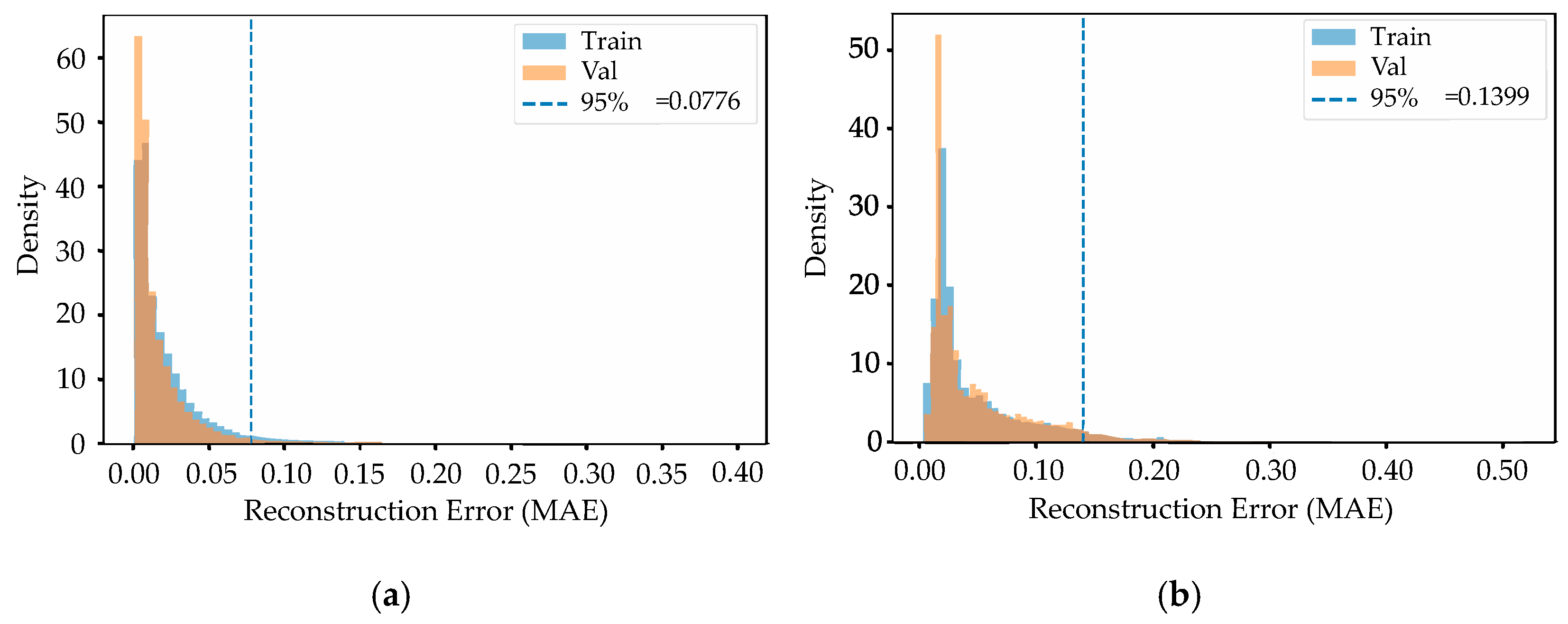
Anomaly scores are typically defined as window-level reconstruction errors, reflecting the degree of deviation between input data and a model’s “normal patterns”. To analyze the overall distribution characteristics of anomaly scores (i.e., the average reconstruction error per window), key quantiles (P50, P90, P95, P99) and the maximum values were calculated for both the overall dataset and feature-specific categories of each battery, as summarized in Table 6. In addition, histograms of the overall reconstruction error distributions for the two feature types are presented in Figure 6.
The anomaly score distributions of all three batteries exhibit a right-skewed long-tail pattern, with the majority of reconstruction errors under normal operating conditions concentrated in the interval [0.02, 0.05], which is far below the threshold. This indicates that the model maintains a low error level and good stability in distinguishing normal conditions, while providing clear separability for abnormal conditions. As a result, it can effectively reduce false alarm rates and enhance the reliability of anomaly warnings in practical applications.

3.2.3. Top-K Anomaly Stability

To evaluate the stability of anomaly detection results across different batteries, multiple models were trained with different random seeds; this study employed the Jaccard similarity coefficient (Jaccard index) [38,39] to measure the overlap of anomalous samples obtained under different random seeds. The average Jaccard values were then computed for the Top 1% and Top 5% anomaly samples, reflecting the stability of the models in identifying extreme anomalies and high-risk regions.
J a c c a r d A , B = | A B | | A B |
The stability results presented in Table 7 reveal a clear contrast between discharging and charging feature types. For discharging, the Top 5% Jaccard coefficients remained consistently high, ranging from 0.84 to 0.89 across all three batteries. This indicates that the model reliably identified high-risk anomaly regions and maintained stable detection performance despite variations in random initialization. By comparison, the charging feature type showed only moderate stability, with Top 5% values between 0.58 and 0.70. The lower consistency suggests that anomaly patterns under charging conditions were less distinct, making them more susceptible to seed-level perturbations.
The Top 1% results exhibit greater variability for both feature types, which is expected given the very limited sample size in this extreme-tail setting. Nonetheless, even under such conditions, discharging features achieved Jaccard values above 0.81 for two of the batteries, confirming that the model remained capable of capturing the most critical anomalies. Overall, the findings highlight that the CNN–LSTM–Attention model demonstrates strong and robust stability in discharging scenarios, while stability in charging conditions is weaker but still within an acceptable range for practical applications.
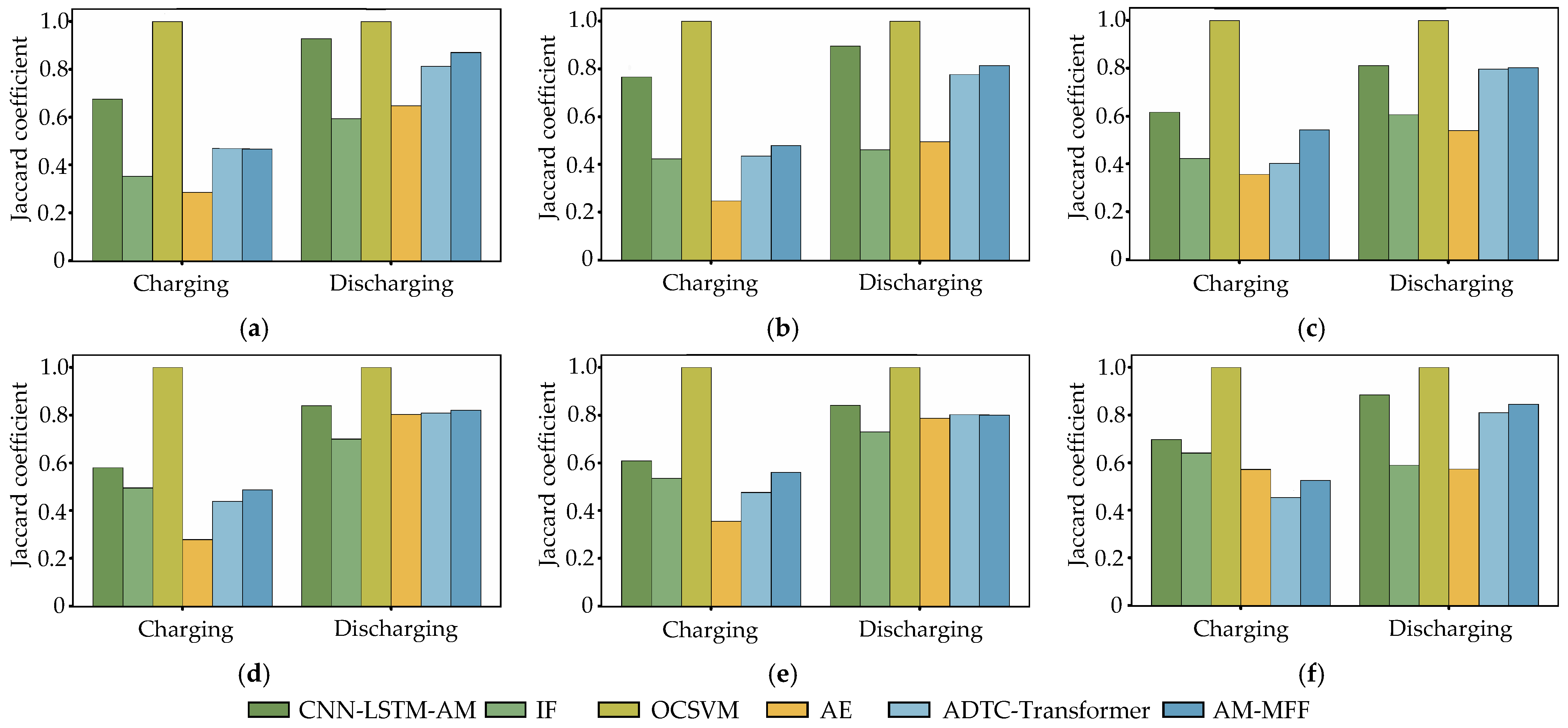
The stability results of different anomaly detection methods are presented in Table 8 and illustrated in Figure 7. As expected, the Jaccard coefficient of OCSVM remained at 1.0 across all batteries and feature types. This outcome stems from the framework’s convex optimization formulation, which produces identical results under different random seeds. Although such determinism yields numerically perfect stability, it does not reflect superior detection capability, as OCSVM lacks the flexibility to capture complex temporal dependencies and often overlooks anomalous samples.
In contrast, the CNN–LSTM–Attention model achieved the most balanced performance. Its average Jaccard coefficient in the Top 5% range was approximately 0.74, and it outperformed classical frameworks such as Isolation Forest and autoencoder, which exhibited lower stability and larger fluctuations under random initialization. The advanced models, ADTC-Transformer and AM-MFF, demonstrated competitive performance but were less consistent across batteries and feature types. ADTC-Transformer achieved moderate stability, while AM-MFF occasionally reached high values but also showed substantial variability.
Overall, the CNN–LSTM–Attention model demonstrated the strongest stability in identifying high-risk anomaly regions. Unlike OCSVM, its stability is achieved through robust feature learning rather than deterministic outputs, and compared with both classical and advanced baselines, it maintains a favorable balance between sensitivity, adaptability, and consistency under real-world variability.

3.2.4. Attention Visualization and Interpretability

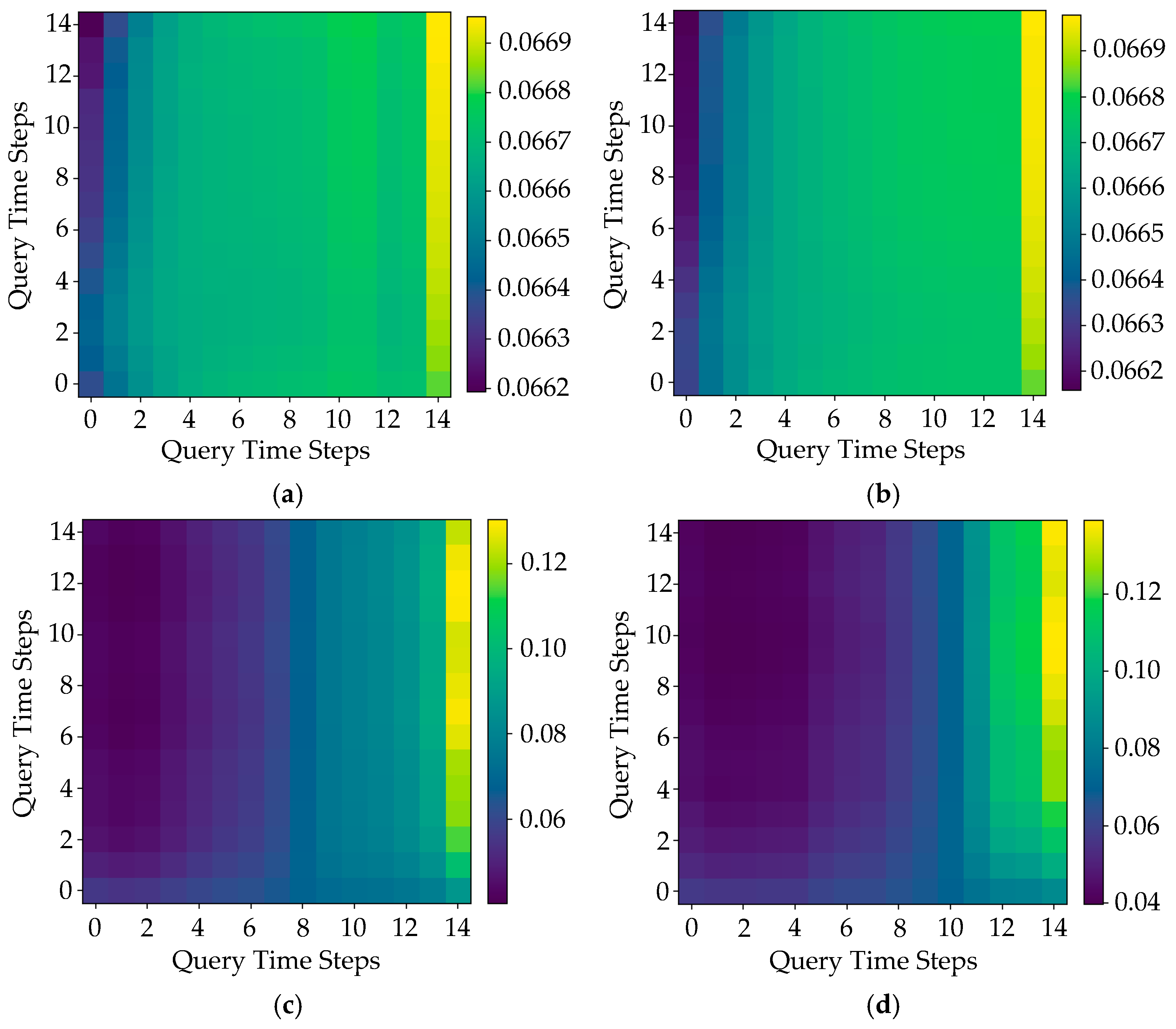
To investigate the interpretability of the CNN–LSTM–Attention model, we visualized the attention weight matrices for representative normal and abnormal windows under both discharging and charging feature types. Each window corresponded to 30 s of operational data (down-sampled to 15 time steps after convolution and pooling). The heatmaps in Figure 8 illustrate how the model allocated attention across different temporal positions.
For discharging features, abnormal windows showed stronger attention concentration in the final few time steps, which coincided with sudden voltage drops and temperature rises. In contrast, the normal windows exhibited smoother distribution without sharp peaks.
For charging features, attention weights also increased toward the later steps, reflecting the model’s natural focus on the end phase of charging where SOC and voltage dynamics became more pronounced. However, the abnormal windows demonstrated a much sharper focus in the last three steps, highlighting the anomaly related segments.
These results confirm that the attention mechanism not only improves anomaly detection accuracy but also enhances model interpretability by explicitly indicating which temporal segments contribute most to decisions.

4. Discussion

In this study, we propose a hybrid CNN–LSTM–Attention model for anomaly detection in lithium-ion batteries of electric bicycles. The results confirm that the integration of convolutional, recurrent, and attention layers provides complementary strengths: the CNN captures local fluctuations in voltage and temperature, LSTM models long-term temporal dependencies, and the attention mechanism highlights critical time steps around anomaly occurrences. Together, these components yield stable reconstruction behavior and more reliable anomaly identification than classical machine learning methods and recently proposed deep models.
The comparative evaluation provides further insights. Traditional approaches, namely Isolation Forest, One-Class SVM, and autoencoder often achieved low distributional distances between training and validation sets, but this was largely due to underfitting and limited capacity to model complex patterns. The advanced architectures, ADTC-Transformer and AM-MFF, showed stronger representational power but exhibited larger variability across batteries. By contrast, the CNN–LSTM–Attention framework achieved a favorable balance between sensitivity, stability, and computational efficiency. In practical terms, this balance translates to more consistent alarm rates across charging and discharging conditions and lower false alarm risk, which is essential for deployment in battery management systems.
Limitations: Despite these advantages, several limitations must be acknowledged. The dataset used in this study contains only ten batteries of the same type and application context, which restricts generalizability across chemistries and platforms. In particular, the model has not yet been validated on other battery types such as LiFePO4, NMC, and solid-state batteries, where degradation behaviors and anomaly patterns may differ. Furthermore, although a cross-battery split was adopted to ensure independence between training and testing, more robust evaluation schemes such as k-fold cross-validation or leave-one-battery-out validation should be applied in future studies to further assess stability and reliability. In addition, the data lacked explicit anomaly labels, making it impossible to calculate precision, recall, or F1-score; performance evaluation therefore relied on reconstruction error distributions and stability metrics rather than standardized supervised benchmarks.
Future directions: Two aspects are particularly critical for improvement. First, incorporating small sets of labeled or simulated fault data would enable semi-supervised training and allow benchmarking with standard classification metrics, thereby increasing confidence in detection accuracy. Second, the anomalies identified in this work were statistical deviations, but we did not explicitly map them to physical failure modes such as thermal runaway, internal short circuits, or cell imbalance. Establishing this mapping and aligning anomaly detection outcomes with safety standards such as IEC 62619 and UL 2271 will be essential for enhancing the practical relevance and regulatory compliance of the proposed approach.
Finally, the framework’s computational footprint remains modest, with fewer than 50 k trainable parameters and millisecond-level inference latency, which supports real-time anomaly monitoring. This lightweight design demonstrates potential for both cloud-based analysis and embedded deployment on resource-constrained devices. Future work should build on these strengths by extending validation to diverse chemistries, incorporating transfer and incremental learning for long-term adaptation, and further optimizing the network for on-board applications.

5. Conclusions

In this study, we introduced a hybrid CNN–LSTM–Attention framework for anomaly detection in lithium-ion batteries of electric bicycles. By combining local pattern extraction, long-term dependency modeling, and adaptive attention weighting, the model effectively addresses the nonlinear and non-stationary nature of real-world battery operation data.
The proposed approach demonstrated three main advances. First, it achieved stable reconstruction performance and consistent alarm rates across multiple batteries and operating conditions, confirming its robustness under real-world variability. Second, compared with both classical machine learning baselines and recently proposed deep architectures, it provided a favorable trade-off between accuracy, stability, and computational efficiency. Third, the integration of attention visualization enhanced interpretability by highlighting the temporal segments most relevant to anomalies, which supports more transparent and actionable monitoring outcomes.
Overall, these findings establish the model as a transferable and lightweight unsupervised framework that advances the state of the art in battery anomaly detection. With its compact size and real-time inference capability, it shows strong potential for deployment in both on-board battery management systems and cloud-based health monitoring platforms, thereby contributing to safer and more reliable operation of electric bicycles.

Author Contributions

Conceptualization, Z.S., W.Y. and Y.M.; methodology, W.Y. and Y.M.; formal analysis, Z.S. and Y.S.; writing—original draft preparation, Z.S., W.Y. and Y.M.; writing—review and editing, Y.S. All authors have read and agreed to the published version of the manuscript.

Funding

This research was funded by the National Key R&D Program “Research on Key Technologies and Standards for Standard Digital Evolution (Phase I)” (NO. 2022YFF0608000) and the Eaglet Program Cultivation Project “Deep Learning-Based Research on Risk Monitoring and Prediction of Electric Vehicle Power Battery Packs” (NO. CY2023112) from Zhejiang Provincial Administration for Market Regulation.

Data Availability Statement

The data presented in this study are available on request from the corresponding author.

Conflicts of Interest

The authors declare no conflicts of interest.

References

  1. Chen, Y.; Kang, Y.; Zhao, Y.; Wang, L.; Liu, J.; Li, Y.; Liang, Z.; He, X.; Li, X.; Tavajohi, N.; et al. A review of lithium-ion battery safety concerns: The issues, strategies, and testing standards. J. Energy Chem. 2021, 59, 83–99. [Google Scholar] [CrossRef]
  2. Guo, R.; Lu, L.; Ouyang, M.; Feng, X. Mechanism of the entire overdischarge process and overdischarge-induced internal short circuit in lithium-ion batteries. Sci. Rep. 2016, 6, 30248. [Google Scholar] [CrossRef]
  3. Qian, L.; Yi, Y.; Zhang, W.; Fu, C.; Xia, C.; Ma, T. Revealing the Impact of High Current Overcharge/Overdischarge on the Thermal Safety of Degraded Li-Ion Batteries. Int. J. Energy Res. 2023, 2023, 8571535. [Google Scholar] [CrossRef]
  4. Xie, S.; Gong, Y.; Ping, X.; Sun, J.; Chen, X.; He, Y. Effect of overcharge on the electrochemical and thermal safety behaviors of LiNi0.5Mn0.3Co0.2O2/graphite lithium-ion batteries. J. Energy Storage 2022, 46, 103829. [Google Scholar] [CrossRef]
  5. Yin, T.; Jia, L.; Li, X.; Zheng, L.; Dai, Z. Effect of High-Rate Cycle Aging and Over-Discharge on NCM811 (LiNi0.8Co0.1Mn0.1O2) Batteries. Energies 2022, 15, 2862. [Google Scholar] [CrossRef]
  6. Tran, M.-K.; Fowler, M. A Review of Lithium-Ion Battery Fault Diagnostic Algorithms: Current Progress and Future Challenges. Algorithms 2020, 13, 62. [Google Scholar] [CrossRef]
  7. Samanta, A.; Chowdhuri, S.; Williamson, S.S. Machine Learning-Based Data-Driven Fault Detection/Diagnosis of Lithium-Ion Battery: A Critical Review. Electronics 2021, 10, 1309. [Google Scholar] [CrossRef]
  8. Zhang, J.; Wang, Y.; Jiang, B.; He, H.; Huang, S.; Wang, C.; Zhang, Y.; Han, X.; Guo, D.; He, G.; et al. Realistic fault detection of li-ion battery via dynamical deep learning. Nat Commun 2023, 14, 5940. [Google Scholar] [CrossRef]
  9. Fan, Y.; Huang, Z.; Li, H.; Yuan, W.; Yan, L.; Liu, Y.; Chen, Z. Fault detection for Li-ion batteries of electric vehicles with feature-augmented attentional autoencoder. Sci. Rep. 2025, 15, 18534. [Google Scholar] [CrossRef] [PubMed]
  10. Zhang, Z.; Ma, J.; Ma, Y.; Gong, X.; Xiangli, K.; Zhao, X. Identification of voltage abnormality in the battery system based on fusion of multiple sparse data observers for real-world electric vehicles. J. Energy Storage 2025, 114, 115727. [Google Scholar] [CrossRef]
  11. Nazim, M.S.; Jang, Y.M.; Chung, B. Machine Learning Based Battery Anomaly Detection Using Empirical Data. In Proceedings of the 2024 International Conference on Artificial Intelligence in Information and Communication (ICAIIC), Osaka, Japan, 19–22 February 2024; pp. 847–850. [Google Scholar]
  12. Sharapatov, A.; Saduov, A.; Assirbek, N.; Abdyrov, M.; Zhumabayev, B. Prediction of rare and anomalous minerals using anomaly detection and machine learning techniques. Appl. Comput. Geosci. 2025, 26, 100250. [Google Scholar] [CrossRef]
  13. Lu, X.-Q.; Tian, J.; Liao, Q.; Xu, Z.-W.; Gan, L. CNN-LSTM based incremental attention mechanism enabled phase-space reconstruction for chaotic time series prediction. J. Electron. Sci. Technol. 2024, 22, 100256. [Google Scholar] [CrossRef]
  14. Chen, H.; Wang, K.; Zhao, M.; Chen, Y.; He, Y. A CNN-LSTM-attention based seepage pressure prediction method for Earth and rock dams. Sci. Rep. 2025, 15, 12960. [Google Scholar] [CrossRef]
  15. Tayeh, T.; Aburakhia, S.; Myers, R.; Shami, A. An Attention-Based ConvLSTM Autoencoder with Dynamic Thresholding for Unsupervised Anomaly Detection in Multivariate Time Series. Mach. Learn. Knowl. Extr. 2022, 4, 350–370. [Google Scholar] [CrossRef]
  16. Qazi, H.; Kaushik, B.N. A Hybrid Technique using CNN LSTM for Speech Emotion Recognition. Int. J. Eng. Adv. Technol. 2020, 9, 1126–1130. [Google Scholar] [CrossRef]
  17. Borre, A.; Seman, L.O.; Camponogara, E.; Stefenon, S.F.; Mariani, V.C.; Coelho, L.d.S. Machine Fault Detection Using a Hybrid CNN-LSTM Attention-Based Model. Sensors 2023, 23, 4512. [Google Scholar] [CrossRef] [PubMed]
  18. Wahid, A.; Breslin, J.G.; Intizar, M.A. Prediction of Machine Failure in Industry 4.0: A Hybrid CNN-LSTM Framework. Appl. Sci. 2022, 12, 4221. [Google Scholar]
  19. Gamaleldin, W.; Attayyib, O.; Alnfiai, M.M.; Alotaibi, F.A.; Ming, R. A hybrid model based on CNN-LSTM for assessing the risk of increasing claims in insurance companies. PeerJ Comput. Sci. 2025, 11, e2830. [Google Scholar] [CrossRef]
  20. Jiang, Y.; Chen, Y.; Yang, F.; Peng, W. State of health estimation of lithium-ion battery with automatic feature extraction and self-attention learning mechanism. J. Power Sources 2023, 556, 232466. [Google Scholar] [CrossRef]
  21. Ouyang, J.; Lin, Z.; Hu, L.; Fang, X. Voltage faults diagnosis for lithium-ion batteries in electric vehicles using optimized graphical neural network. Sci. Rep. 2025, 15, 27328. [Google Scholar] [CrossRef]
  22. Shi, D.; Zhao, J.; Wang, Z.; Zhao, H.; Wang, J.; Lian, Y.; Burke, A.F. Spatial-Temporal Self-Attention Transformer Networks for Battery State of Charge Estimation. Electronics 2023, 12, 2598. [Google Scholar] [CrossRef]
  23. Hussein, H.M.; Esoofally, M.; Donekal, A.; Rafin, S.M.S.H.; Mohammed, O. Comparative Study-Based Data-Driven Models for Lithium-Ion Battery State-of-Charge Estimation. Batteries 2024, 10, 89. [Google Scholar] [CrossRef]
  24. Yamashita, R.; Nishio, M.; Do, R.K.G.; Togashi, K. Convolutional neural networks: An overview and application in radiology. Insights Imaging 2018, 9, 611–629. [Google Scholar] [CrossRef]
  25. Hochreiter, S.; Schmidhuber, J. Long short-term memory. Neural Comput. 1997, 9, 1735–1780. [Google Scholar] [CrossRef]
  26. Greff, K.; Srivastava, R.K.; Koutník, J.; Steunebrink, B.R.; Schmidhuber, J. LSTM: A search space odyssey. IEEE Trans. Neural Netw. Learn. Syst. 2016, 28, 2222–2232. [Google Scholar] [CrossRef] [PubMed]
  27. Madani, S.S.; Ziebert, C.; Vahdatkhah, P.; Sadrnezhaad, S.K. Recent Progress of Deep Learning Methods for Health Monitoring of Lithium-Ion Batteries. Batteries 2024, 10, 204. [Google Scholar] [CrossRef]
  28. IEC 62660-1; Secondary Lithium-Ion Cells for the Propulsion of Electric Road Vehicles—Part 1: Performance Testing. International Electrotechnical Commission: Geneva, Switzerland, 2018.
  29. IEC 62660-2; Secondary Lithium-Ion Cells for the Propulsion of Electric Road Vehicles—Part 2: RELIABILITY and Abuse Testing. International Electrotechnical Commission: Geneva, Switzerland, 2018.
  30. GB/T 36972-2018; Lithium-Ion Battery for Electric Bicycle. Administration for Market Regulation of the People’s Republic of China. Standardization Administration of the People’s Republic of China: Beijing, China, 2018.
  31. Lee, J.; Wang, L.; Jung, H.; Lim, B.; Kim, D.; Liu, J.; Lim, J. Deep Neural Network with Anomaly Detection for Single-Cycle Battery Lifetime Prediction. Batteries 2025, 11, 288. [Google Scholar] [CrossRef]
  32. Goldstein, M.; Uchida, S. A Comparative Evaluation of Unsupervised Anomaly Detection Algorithms for Multivariate Data. PLoS ONE 2016, 11, e0152173. [Google Scholar] [CrossRef]
  33. Mejri, N.; Lopez-Fuentes, L.; Roy, K.; Chernakov, P.; Ghorbel, E.; Aouada, D. Unsupervised anomaly detection in time-series: An extensive evaluation and analysis of state-of-the-art methods. Expert Syst. Appl. 2024, 256, 124922. [Google Scholar] [CrossRef]
  34. González-Muñiz, A.; Díaz, I.; Cuadrado, A.A.; García-Pérez, D.; Pérez, D. Two-step residual-error based approach for anomaly detection in engineering systems using variational autoencoders. Comput. Electr. Eng. 2022, 101, 108065. [Google Scholar] [CrossRef]
  35. Lachekhab, F.; Benzaoui, M.; Tadjer, S.A.; Bensmaine, A.; Hamma, H. LSTM-Autoencoder Deep Learning Model for Anomaly Detection in Electric Motor. Energies 2024, 17, 2340. [Google Scholar] [CrossRef]
  36. Massey, F.J., Jr. The Kolmogorov-Smirnov test for goodness of fit. J. Am. Stat. Assoc. 1951, 46, 68–78. [Google Scholar] [CrossRef]
  37. Peyré, G.; Cuturi, M. Computational optimal transport: With applications to data science. Found. Trends® Mach. Learn. 2019, 11, 355–607. [Google Scholar] [CrossRef]
  38. Jaccard, P. Étude comparative de la distribution florale dans une portion des Alpes et des Jura. Bull. Soc. Vaudoise Sci. Nat. 1901, 37, 547–579. [Google Scholar]
  39. Real, R.; Vargas, J.M. The probabilistic basis of Jaccard’s index of similarity. Syst. Biol. 1996, 45, 380–385. [Google Scholar] [CrossRef]
Figure 1. CNN–LSTM–Attention model flowchart.
Batteries 11 00384 g001
Figure 2. Comparison of average alarm rate under different hyperparameter settings.
Batteries 11 00384 g002
Figure 3. Stability analysis under different hyperparameter settings. (a) Top 1% Jaccard (mean ± std) comparison. (b) Top 5% Jaccard (mean ± std) comparison.
Batteries 11 00384 g003
Figure 4. Threshold sensitivity analysis results.
Batteries 11 00384 g004
Figure 5. Training and validation loss curves for (a) discharging features and (b) charging features.
Batteries 11 00384 g005
Figure 6. Overall reconstruction error distributions for batteries (a) 342421544, (b) 342425605, and (c) 342429831.
Batteries 11 00384 g006
Figure 7. Top-K stability comparison of anomaly detection methods across three batteries and two feature types. The Jaccard coefficient is used as the stability metric. (a) Battery 342421544 under Top 1% setting. (b) Battery 342425605 under Top 1% setting. (c) Battery 342429831 under Top 1% setting. (d) Battery 342421544 under Top 5% setting. (e) Battery 342425605 under Top 5% setting. (f) Battery 342429831 under Top 5% setting.
Batteries 11 00384 g007
Figure 8. Attention heatmaps of the CNN–LSTM–Attention model. (a) Discharging feature type, abnormal window. (b) Discharging feature type, normal window. (c) Charging feature type, abnormal window. (d) Charging feature type, normal window.
Batteries 11 00384 g008
Table 1. Description of the dataset items used in the experiment.
TypeParameterDescription
Discharging
Features
batVDischarge voltage
batIDischarge current
temp1Temperature sensor 1
temp2Temperature sensor 2
useUpWhAccumulated discharge energy
dischargeHTempMaximum discharge temperature
dischargeLTempMinimum discharge temperature
shortCircuitCountNumber of short circuits
Charging
Features
batteryUCharging voltage
batteryICharging current
batterySocState of charge
batteryUseUpWhAccumulated charging energy
tempTemperature sensor
chargeStateCharging state
chargeStatusCharging mode
safePowerSafe power
Table 2. Generalization validation parameters of training and validation sets.
Feature TypeKS StatisticWasserstein Distance95% Threshold
Discharging0.10270.0049000.0776
Charging0.11040.0024400.1399
Table 3. Parameter settings for generalization verification of traditional anomaly detection methods.
Feature TypeMethodKS StatisticWasserstein Distance
DischargingAE0.00300.0000
IF0.00350.0002
OCSVM0.00322.0140
ADTC-Transformer0.14260.0132
AM-MFF0.17520.0107
ChargingAE0.00460.0001
IF0.00360.0003
OCSVM0.00562.0703
ADTC-Transformer0.12030.0095
AM-MFF0.18010.0088
Table 4. Thresholds and alarm rates on the test set.
Battery IDCharging FeaturesDischarging FeaturesOverall Alarm Rate
ThresholdAlarm RateThresholdAlarm Rate
3424215440.07764.88%0.13995.04%4.96%
3424256050.07765.16%0.13995.27%5.21%
3424298310.07765.00%0.13995.17%5.09%
Table 5. Alarm rates of traditional anomaly detection methods.
Battery IDTypeAEIFOCSVMADTCAM-MFF
342421544Discharging2.34%3.96%2.54%5.86%6.03%
Charging1.47%4.23%1.70%6.74%8.61%
342425605Discharging5.70%6.47%4.97%6.55%7.10%
Charging0.41%2.31%1.00%6.59%6.61%
342429831Discharging10.89%2.65%7.34%7.76%7.06%
Charging1.97%6.38%2.13%7.68%6.82%
Overall Alarm Rate3.80%4.33%3.28%6.87%7.04%
Table 6. Distribution characteristics of window-level mean reconstruction errors.
Battery IDTypeP50P90P95P99MaxRemarks
342421544Overall0.03710.06120.07450.10130.2824Right-skewed distribution with moderate tail
Discharging 0.0743 Close to threshold
Charging 0.1400 Slightly above threshold
342425605Overall0.03800.06310.07660.10480.2975Right-skewed distribution with short tail
Discharging 0.0764 Close to threshold
Charging 0.1406 Slightly above threshold
342429831Overall0.03750.06180.07490.10250.2896Right-skewed distribution with high concentration
Discharging 0.0748 Below threshold
Charging 0.1398 Close to threshold
Table 7. Jaccard coefficients on the test set.
Battery IDTypeTop 1%Top 5%
342421544Discharging0.9285910.840445
Charging0.6762730.580456
342425605Discharging0.8967210.841555
Charging0.7661080.609360
342429831Discharging0.8109420.885450
Charging0.6162400.697611
Table 8. Jaccard coefficients of classical methods.
Battery IDTypeMethodTop 1%Top 5%
342421544DischargingIF0.59410.7005
OCSVM1.00001.0000
AE0.64840.8050
ADTC-Transformer0.81310.8097
AM-MFF0.87060.8213
ChargingIF0.35310.4963
OCSVM1.00001.0000
AE0.28500.2791
ADTC-Transformer0.46930.4386
AM-MFF0.46610.4868
342425605DischargingIF0.46270.7303
OCSVM1.00001.0000
AE0.49600.7884
ADTC-Transformer0.77660.8027
AM-MFF0.81480.8014
ChargingIF0.42290.5367
OCSVM1.00001.0000
AE0.24680.3561
AM-MFF0.48010.5606
CNN-LSTM-AM0.81090.8854
342429831DischargingIF0.60660.5896
OCSVM1.00001.0000
AE0.54010.5736
ADTC-Transformer0.79770.8098
AM-MFF0.80300.8456
ChargingIF0.42310.6407
OCSVM1.00001.0000
AE0.35650.5719
ADTC-Transformer0.40290.4537
AM-MFF0.54320.5252
Disclaimer/Publisher’s Note: The statements, opinions and data contained in all publications are solely those of the individual author(s) and contributor(s) and not of MDPI and/or the editor(s). MDPI and/or the editor(s) disclaim responsibility for any injury to people or property resulting from any ideas, methods, instructions or products referred to in the content.