A Resource-Constrained Polynomial Regression Approach for Voltage Measurement Compression in Electric Vehicle Battery Packs

Abstract

Technologies like data-driven methods for battery state estimation, fleet monitoring and cloud-based BMSs are emerging. However, challenges in data compression and storage hinder their widespread adoption. This paper addresses these issues by proposing a novel, efficient lossy voltage data compression method for measurements in electric vehicles. The method is grounded in polynomial regression and enables the use of the adaptive method without the need for parameters or training of the model which, representing an improvement over existing techniques. At a compression rate of 99.75% in an ambient temperature of 25 °C on average across all drive cycles compared, the root mean square error (RMSE) was 5.62 mV. Impressively, at a compression rate of 99%, the RMSE decreased to 3.12 mV. Furthermore, an implementation on a low-power STM32 microcontroller can compress 600 data points in just 35 milliseconds, demonstrating its suitability for real-time applications. These results highlight the potential of our approach to significantly improve the efficiency and accuracy of voltage measurement compression in electric vehicles, paving the way for advancements in electric vehicle technology.

1. Introduction

In the research field of batteries for electric vehicles, data-driven methods for estimating states, such as the state of charge (SOC), State of Health (SOH), or core temperature, are becoming increasingly relevant [1,2,3]. Furthermore, technologies such as monitoring, digital twins, and cloud-based battery management systems (BMSs) are raising interest from researchers and the industry [4,5,6]. A battery pack contains a large number of battery cells connected in a series and in parallel to meet the requirements of high-energy storage [7]. Each of these cells has to be monitored and controlled. Many problems must be solved before these data-driven technologies can be applied to electric vehicles (EVs). A primary focus is currently on the development of high-accuracy estimation models. However, efficient data compression is needed to transfer and store data in the field of the Internet of Things (IoT) with increasing data amounts [8]. Data compression also decreases the requirements of resources such as storage, bandwidth, and energy consumption in data storage and transfer [9].

Khalid Sayood [10] describes compression as the science of representing data in a packed condition. Data compression consists of two parts: compression, which encodes the data, and decompression, which decodes the data. The different compression techniques can be classified as lossless and lossy methods.

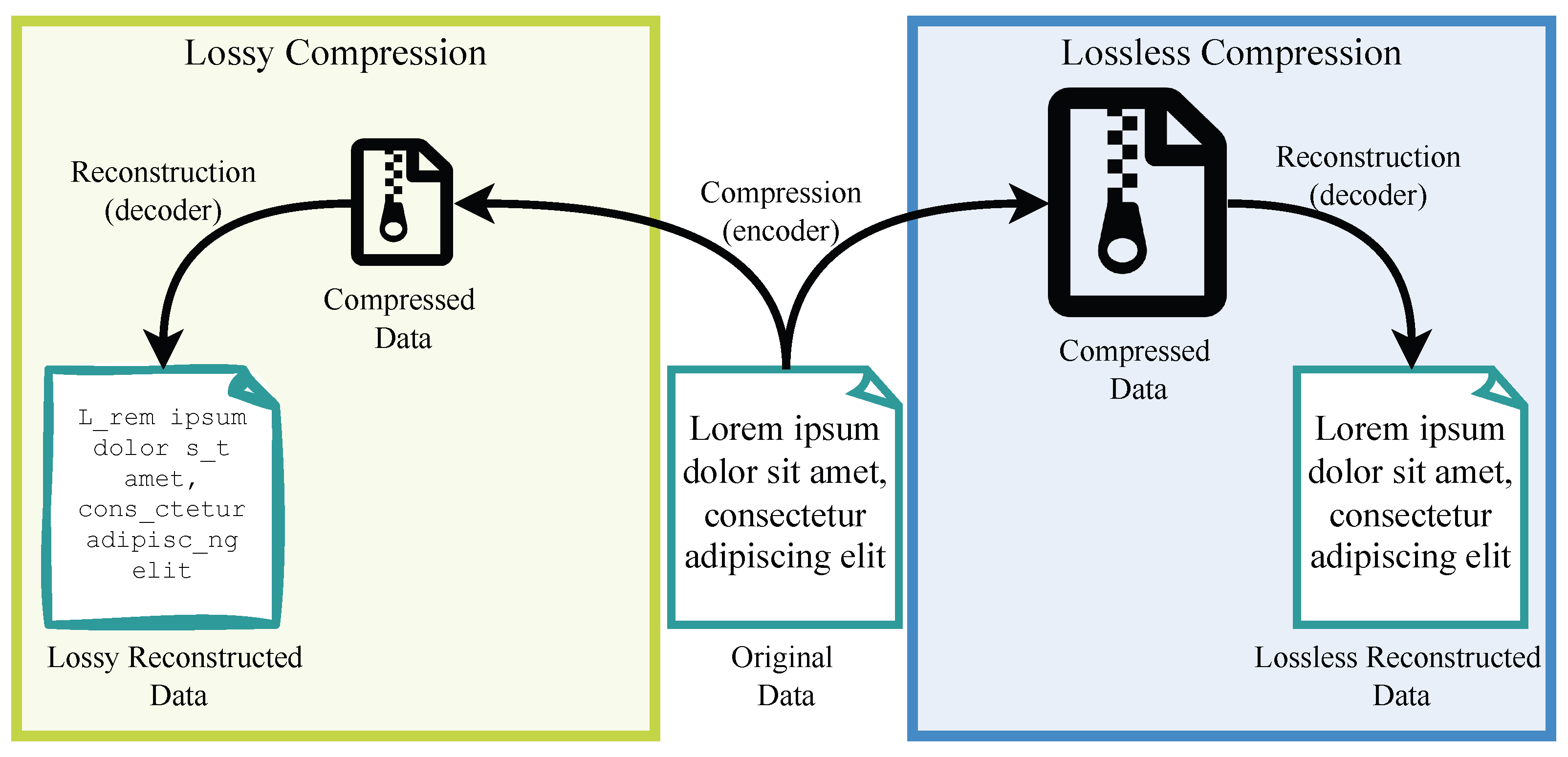
Figure 1 illustrates the difference between both methods. With lossless techniques, compressed data can be exactly reconstructed to match the original data. These methods are usually used for data that cannot be changed due to compression, such as documents or database entries. This kind of compression is limited by the maximum amount of data that can be compressed without loss. Within the figure, the loss of information is depicted by an underscore in the text, a variation in font style, and a schematic representation of the file icon. Chiarot and Silvestri [11] show additional categories to describe compression algorithms:

• Non-adoptive and adaptive algorithms: A model’s training is required to compress the data efficiently or not. Non-adoptive algorithms are dependent on model training.
• Symmetric and non-symmetric: The algorithm is symmetric if the decoder performs the same operations, such as the encoder, but in reverse order.

Figure 1. The process of compression and decompression of lossless and lossy compression methods; data loss illustrated by font change and underscores in the data text.

Figure 1. The process of compression and decompression of lossless and lossy compression methods; data loss illustrated by font change and underscores in the data text.

One main attribute used to evaluate and compare different compression methods is the Compression Ratio ($CR$) and Rate of Compression ($RoC$). This attribute quotes the ratio between the original amount of data and the compressed amount [12]:

$$\begin{array}{cc}\hfill CR& ={\displaystyle \frac{\mathrm{Compressed}\mathrm{Size}}{\mathrm{Original}\mathrm{Size}}},\hfill \end{array}$$

(1)

$$\begin{array}{cc}\hfill RoC& =1-CR\hfill \end{array}$$

(2)

The lossy compression’s archive achieves a much higher CR than the lossless compression’s, but a the cost of a loss in accuracy of the reconstructed data [13]. Alternatively, as described in the literature [9], the decompressed data of lossy compression methods approximate the original data. In addition to CR, the precision after decompression is an attribute of these methods. Accuracy can be described in metrics such as Mean Absolute Error (MAE) and Root Mean Square Error (RMSE) [14].

The domain of various lossy compression techniques is extensive. Correa [9] identifies several lossy compression techniques, facilitating differentiation among them:

• Transform: changing the domain of the signal, such as from the time to the frequency domain by Fourier Transform.
• Artificial Intelligence (AI): one use case of AI is the use of neuronal networks as encoders and decoders to compress and decompress data.
• Interpolation: creating new data points using a range of known points is the definition of interpolation. With this method, data can be reconstructed on the basis of approximate or representative values.
• Hybrid: The combination of lossy and lossless algorithms.

See [15]’s remarks on the estimation of battery cell state as one of the key functionalities of BMSs. Therefore, measured data, such as current and voltage, must be processed and stored. Especially for the usage in second-life applications, historical data are necessary. Computational and storage resources are highly limited regarding BMS applications. This necessitates the implementation of both efficacious and robust data compression methodologies. In addition to lossless compression methods, the required amount of data storage can be reduced by variable recording frequency depending on the dynamics of the battery pack [16]. Therefore, the authors propose an algorithm to reduce the recording frequency depending on the dynamics of the battery cell. According to the results of the paper, the accuracy highly depends on the frequency. A recording frequency of 2 $\mathrm{Hz}$ is required to enable accurate estimations during high dynamic processes. Based on this work, Zhou [17] suggests a data storage approach that utilizes the frequency division model of a battery pack to reconstruct the voltage data that has been logged with a lower frequency. A recording frequency of $0.2$ $\mathrm{Hz}$ enabled compression to 28% of the original required space with a mean RMSE of $9.7$ $\mathrm{m}$$\mathrm{V}$ on eight tested battery cells.

To address the compression of voltage data, Tang et al. [18] propose a method that blends a battery model, a neuronal network-based migration model, and interpolation. A RoC of 90%, 95%, and 99% ends in a reconstructed RMSE of $2.9$ $\mathrm{m}$$\mathrm{V}$, $4.16$ $\mathrm{m}$$\mathrm{V}$, and $10.01$ $\mathrm{m}$$\mathrm{V}$.

It turns out that the compression methods presented so far are dependent on battery parameters being estimated or ML models being trained beforehand. Cell aging, temperature changes, and the state of charge strongly influence the behavior of batteries and influence the accuracy of battery models and their parameters [19]. This suggests that an adaptive method, which is independent of environmental variables, is better suited for use in real-work applications.

Polynomial coding has been established as a lossy compression method in the field of image and speech compression for a long time [20,21,22]. This paper introduces a method to compress and reconstruct voltage measurements using a lossy polynomial coding algorithm. The algorithm’s focus is on accuracy and lightweight computation. Therefore, the current of series-connected battery cells can be utilized to reconstruct the voltage using the polynomial regression parameters of each individual cell. This work introduces and evaluates this method. Resource-saving decompression is particularly important when it comes to an application in the BMS. Here, bandwidths and computing power are highly limited. Massive resource savings can also be achieved for the storage of measurements in cloud infrastructures on a fleet scale.

To the best of our knowledge, this paper presents the first adaptive approach to compress voltage data. To compress voltage data, a polynomial coding method is proposed. The characteristics of our proposed method are as follows:

• Adaptive method: the method is able to adjust to changing battery conditions.
• No battery-specific parameters required for compression: the method does not require prior knowledge of battery characteristics.
• No machine learning training: the method does not need to be trained on specific datasets.
• Computational efficiency: the method is computationally efficient, making it suitable for real-time applications for implementation on standard BMSs.

2. Compression Method

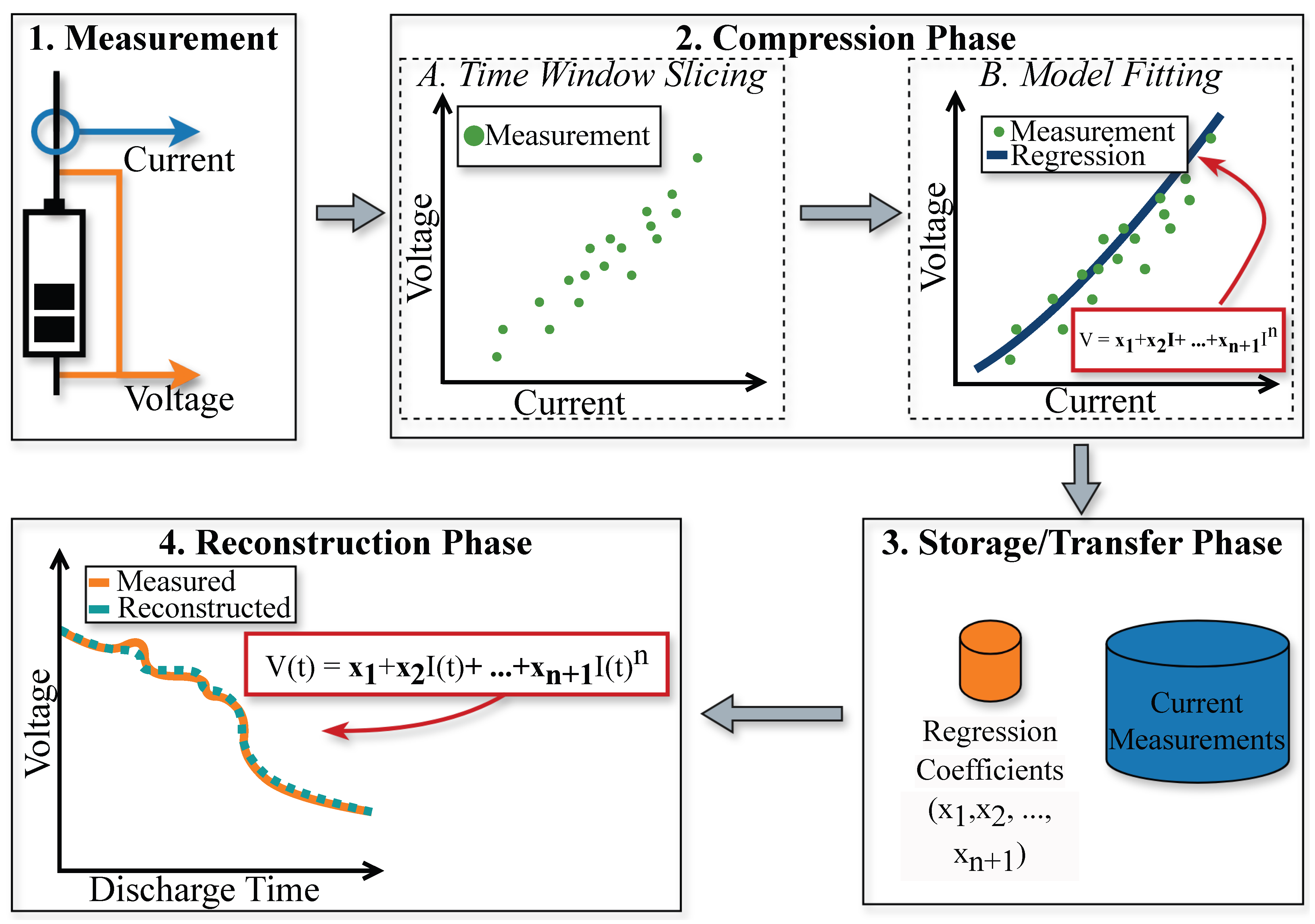
The proposed method contains four phases: measurement, compression, transfer and storage, and reconstruction. The phases are illustrated in Figure 2.

An overview of the individual steps is provided before the method is explained in detail:

• Measurement: the voltage and current measurement of the battery cell.
• Compression: the compression of the measured values consists of two sub-phases:
  • Time window slicing: slicing the measurement values into time frames. The fixed length of the time frames is named the window size.
  • Model fitting: fitting the polynomial regression. It is the regression of the current and voltage measurements.
• Storage/Transfer: to transfer and store the compressed measurements, only the regression coefficients and the values of the current measurement must be stored.
• Reconstruction: the voltage values are reconstructed based on the regression coefficients and the time-dependent current values.

The proposed method primarily focuses on compression and reconstruction, with the additional, albeit essential, steps of measuring and storing/transferring. In the context of the work presented here, the measurement method used is not relevant; the accuracy and efficiency of the method are independent of it. Furthermore, the procedure is also independent of the storage method used. Effective compression is necessary if the data are stored exclusively on the vehicle or transferred, processed, and stored in the cloud. The installed bandwidth within the vehicle and storage capacity can be utilized more effectively. If the measurement data are to be transferred to the cloud, bandwidth can be utilized effectively, and costs can be reduced.

2.1. Compression

Multiple studies have shown that the fitting of a voltage relaxation curve can be used to estimate the SOH or capacity of a battery cell [23,24,25]. An equivalent circuit model (ECM) characterizes the behavior of a battery throughout its charging and discharging processes. This model encompasses multiple RC connections. Figure 3 shows an ECM containing n RC components. The internal resistance of the cell is described by $R_0$. Furthermore, $C_k$ and $R_k$ represent the capacitance and resistance of the RC component k, which describes the diffusion process of the battery cell.

Liu [26] defines the battery cell voltage $u_B$ as follows:

$$\begin{array}{cc}\hfill u_B=& V_{oc}\left(SOC\right)-i{R}_0-i{R}_1\left[1-\exp \left({\displaystyle \frac{T}{{\tau }_1}}\right)\right]\hfill \\ \hfill & -i{R}_2\left[1-\exp \left({\displaystyle \frac{T}{{\tau }_2}}\right)\right]-\cdots -i{R}_n\left[1-\exp \left({\displaystyle \frac{T}{{\tau }_n}}\right)\right],\hfill \end{array}$$

(3)

where $V_{ocv}\left(SOC\right)$ is the open-circuit voltage as a function of the SOC, i the current, ${\tau }_k$ the time constant $C_k\times R_k$, and T the discharge/charge time.

Within a short measurement time window, the change of $V_{oc}$ and the changes of T, R, and C can be ignored and seen as fixed values of the function. Due to this, the voltage can be articulated as a function of the current in the following manner:

$$\begin{array}{c}\hfill u_B\approx {\beta }_0+{\beta }_1{i}_B+\cdots +{\beta }_n{i}_B,\end{array}$$

(4)

where ${\beta }_k$ represents the parameter $R_k\left[1-\exp \left({\displaystyle \frac{T}{{\tau }_k}}\right)\right]$ of the RC component k. The parameters of this function can be identified by applying regression analysis.

Thus, regression has to be introduced. Regression is a statistical method to describe the relation between variables [27]. The main goal of regression is to summarize the data as usefully and elegantly as possible [28]. The definition of the simple linear regression model is

$$\begin{array}{c}\hfill y={\beta }_0+{\beta }_{1}x+ϵ,\end{array}$$

(5)

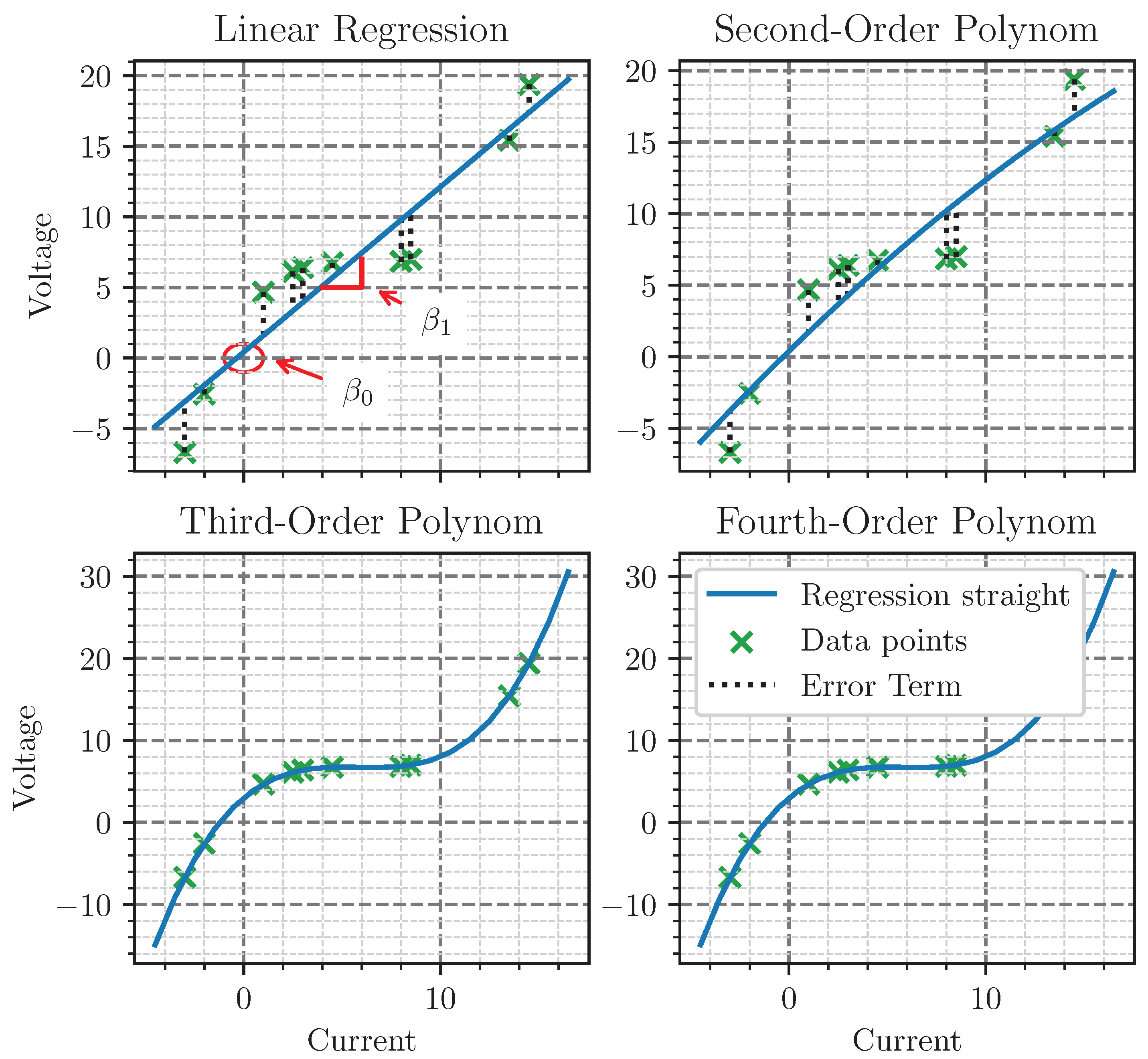
where ${\beta }_0$ is the intercept, ${\beta }_1$ the slope, and $ϵ$ the random component. Figure 4 visualizes, in the top left, an example of linear regression. This figure shows ten data points. The intercept ${\beta }_0$ and the slope ${\beta }_1$ characterize the linear regression.

As the estimation method for the parameters ${\beta }_0$ and ${\beta }_1$, the ordinary least squares method is used, described in [29]. A linear function cannot accurately characterize the relationship between current and voltage over a brief interval. Furthermore, a curved function has to be used to determine the behavior between these two characteristics. To do so, a higher-order polynomial regression model in the $(k+1)$th order is described by Seber [30] as follows:

$$\begin{array}{c}\hfill y={\beta }_0+{\beta }_{1}x+{\beta }_2{x}^2+\cdots +{\beta }_k{x}^k+ϵ.\end{array}$$

(6)

In Figure 4, a second-order (top right), third-order (bottom left), and fourth-order (bottom right) polynomial regression are represented. Polynomial regression allows for describing non-linear processes in a battery over a defined period. As illustrated in Figure 4, higher-order models enable better representation of the relation between current and voltage over a given time. Thus, voltage measurements can be lossy-compressed as a polynomial regression model. For instance, a quartic polynomial model spanning a dataset comprising 100 paired observations of voltage and current facilitates a CR of 95% for the voltage data. This efficiency is achieved as the model is succinctly represented by five coefficients: ${\beta }_1$, ${\beta }_2$, ${\beta }_3$, ${\beta }_4$, and $({\beta }_0+ϵ)$, rather than the complete set of 100 voltage measurements.

The least squares method is applied to estimate the regression parameters. Several detailed descriptions of the parameter estimation of the polynomial regression have been given [31,32].

2.2. Reconstruction

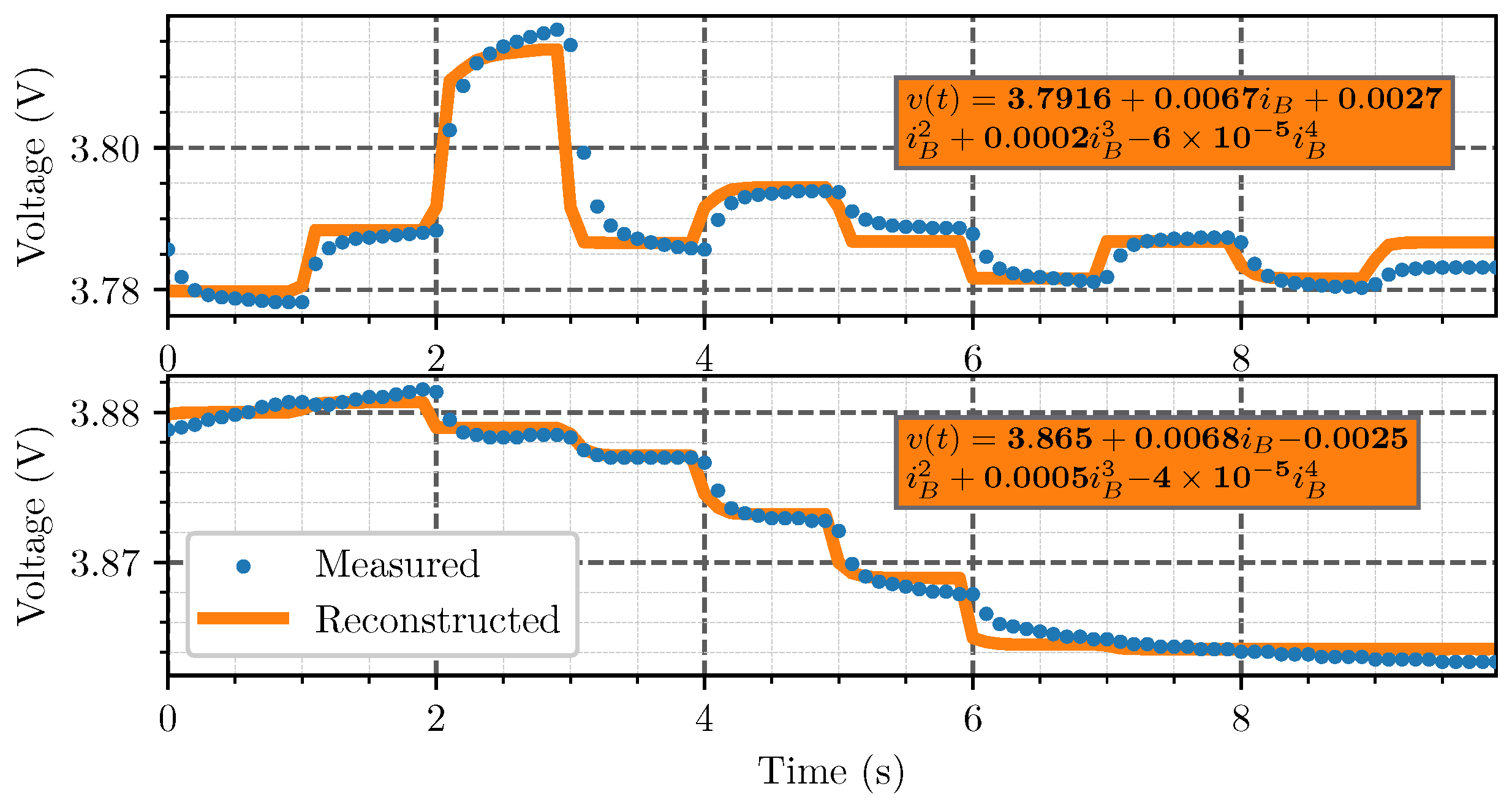
The reconstruction of the adaptive, non-symmetrically lossy-compressed voltage data $u_B\left(t\right)$ was executed utilizing the current values $i\left(t\right)$ and the polynomial coefficients. The function described in Equation (6) was employed for this purpose. Figure 5 depicts the temporal evolution of the reconstructed voltage. The input values are the regression coefficients and the current measurements.

3. Method Analysis and Discussion

The evaluation consists of two parts: accuracy and runtime. Two main factors decide if the method can be utilized, whether the reconstructed data are accurate and whether the method is employable within BMS hardware. Through several datasets, the accuracy of the method was evaluated. The method’s runtime was evaluated with an STM32L432 microcontroller (STMicroelectronics NV, Plan-les-Ouates, Switzerland) as the device under test (DUT). Accuracy and runtime were evaluated independently.

3.1. Accuracy of Lossly Data Compression

Three distinct datasets, two previously published datasets, and an unpublished dataset, were utilized for this to assess the proposed methodological framework’s effectiveness.

• Temperature-dependent constant current (CC)–constant voltage (CV) charging–discharging data:
  for this work, constant current–constant voltage (CC-CV) charging and discharging cycles were performed at various C-rates and ambient temperatures, with a measurement frequency of 1 $\mathrm{Hz}$. As the DUT, eight Li-Ion Molicel P42A battery cells (Molicel, Taipei, Taiwan) were used.
• Aging data:
  Jöst et al. [33] published aging data of 28 18650 high-energy NCA/C+Si round cells measured with a $0.1$ $\mathrm{Hz}$ frequency. Drive cycles were applied to age the cells at an ambient temperature of 25 °C.
• Drive cycle data:
  Kollmeyer [34] published a dataset that includes data from different tests performed as described in the data description. As the DUT, the graphene lithium polymer (LiPo) battery Turnigy Graphene 5000 mAh 65C (HobbyKing, Hong Kong, China) was employed during the tests. The data were measured with a 10 $\mathrm{Hz}$ frequency. To evaluate the proposed lossy data compression method, driving cycle data of the dataset were used. These drive cycles include the Urban Dynamometer Driving Schedule (UDDS), Highway Fuel Economy Test (HWFET), LA92, US06, and random mixes of these drive cycles specified as Mixed1–8. In addition to different drive cycles, six different ambient temperatures were under test.

The accuracy of the presented method depends on the selected order of the polynomial compression, as well as the length of the time window that is compressed. It is imperative to determine the optimal polynomial order necessary to most accurately characterize the correlation between voltage and current. Therefore, in the first step, the effect of the chosen polynomial order on accuracy was evaluated. The Kollmeyer dataset [34] was used with several window sizes and third-, fourth-, fifth-, and sixth-order polynomials for regression.

Table 1. Mean MAE and RMSE depending on polynomial order and window size through full dataset of [34].

Polynomial Order	Window Size	RoC (%)	MAE (mV)	RMSE (mV)
3	50	92	0.67	1.50
3	100	96	1.32	2.87
3	500	99.2	3.93	7.59
3	1000	99.6	5.54	10.17
4	50	90	0.35	0.77
4	100	95	0.94	2.04
4	500	99	3.23	6.44
4	1000	99.5	4.92	9.20
5	50	88	0.16	0.35
5	100	94	0.65	1.40
5	500	98.8	2.74	5.58
5	1000	99.4	4.42	8.36
6	50	86	0.14	0.43
6	100	93	1.05	2.74
6	500	98.6	3.33	8.41
6	1000	99.3	4.61	8.44

shows the mean MAE and RMSE depending on the window size and polynomial order. Furthermore, it shows the resulting RoC.

Due to the high accuracy and RoC shown in Table 1, the following experiments were performed with a fourth-order polynomial regression for compression.

3.1.1. Temperature-Dependent CC-CV Charging–Discharging Data

Figure 6 shows the experimental setup to collect the data for accuracy evaluation of eight cells (green).

The battery testbench consisted of an Ivium (Eindhoven, Netherlands) (Model: OctoStat5000) battery cycler (blue), a Binder (Tuttlingen, Germany) environment control chamber (Model MKF 240) highlighted in red, and a Microsoft (Redmond, Washington, USA) Surface Pro 7 was used for the overall system control and centralized monitoring using the IviumSoft (Version: 4.1165) platform. A cyclindrical Li-Ion Molicel 4200 mAh 45 A INR-21700 was selected as a battery in this study. The battery specifications are as outlined in the manufacturer’s datasheet (https://www.molicel.com/wp-content/uploads/INR21700P42A-V4-80092.pdf, accessed on 2 Feburary 2024).

A series of battery cyclings were performed with a range of ambient temperatures and C-rates during the CC-CV charge/discharge cycles. The list below mentions the performed experiments in order:

• Ambient temperatures: 20 °C 10 °C, 0 °C, $-10$ °C, $-20$ °C, 30 °C, and 40 °C;
• Three× each: 0.3C; 0.5C; 0.8C; and 1C.

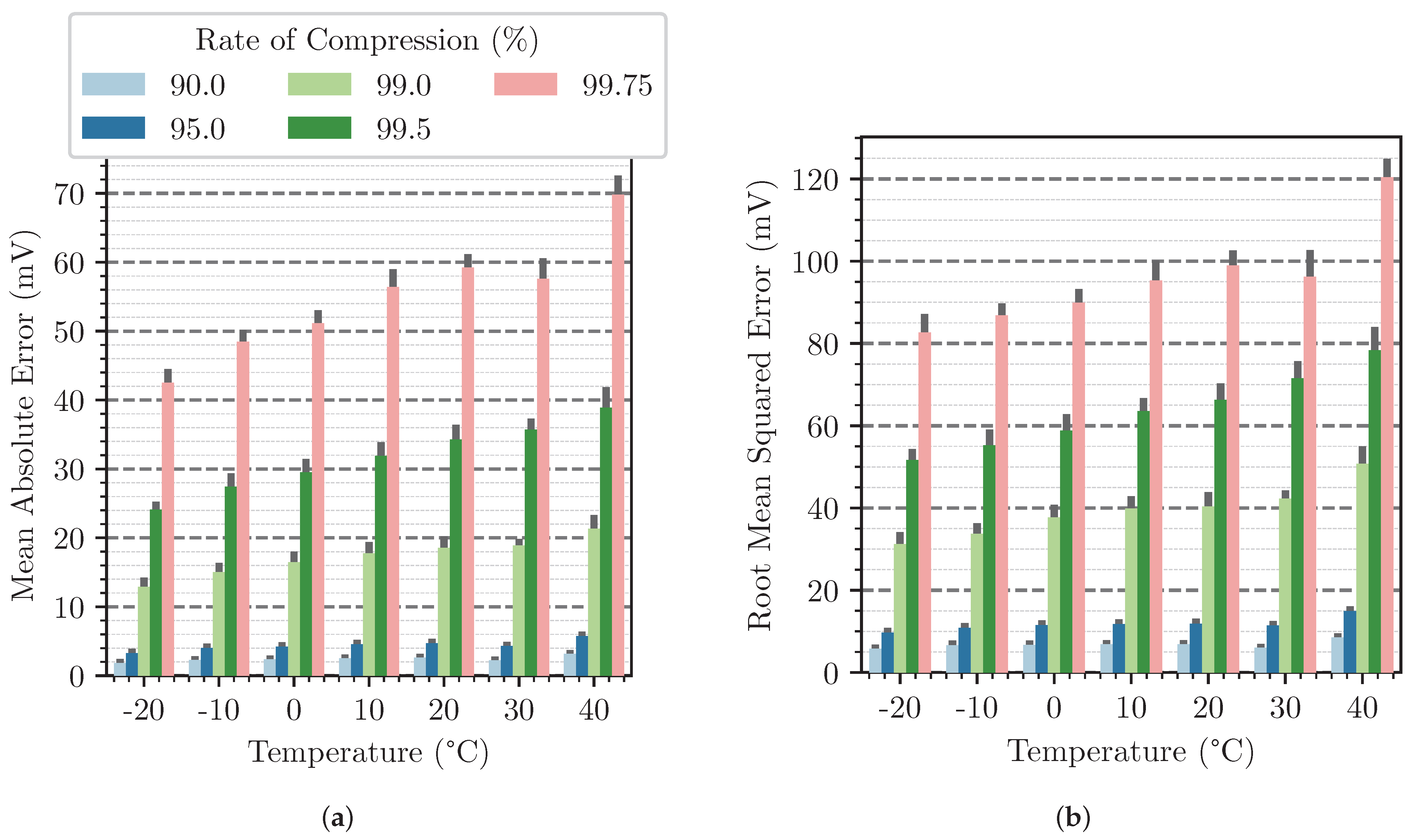
In Figure 7, the MAE (a) and RMSE (b) at ambient temperatures $-20$ °C up to 40 °C are illustrated. The RoCs 90%, 95%, 99%, 99.5%, and 99.75% are performed. The bar plots illustrate the mean accuracy and the standard deviation, illustrated as black error bars.

Across all temperatures, there is an increase in both evaluation metrics by a factor of three or more between the compression rate of 99% and 99.75%. Furthermore, there is a noticeable increase in the error at higher temperatures. For example, a MAE of 2 $\mathrm{m}$$\mathrm{V}$ can be determined from $-20$ °C at a compression of 90%. At 40 °C, this is already $3.8$ $\mathrm{m}$$\mathrm{V}$ with identical compression.

A more detailed analysis, illustrated in Figure 8, shows the cause of the errors. The figure illustrates a 1C CC-CV charge and discharge cycle at an ambient temperature of 20 °C and a RoC of 95%. The graph distinctly elucidates both the advantages and limitations inherent in the methodology. As the voltage is compressed on the basis of the current, accurate compression is not possible at a constant current, as illustrated in the left zoom-in. At constant voltage, a high accurate compression can be seen, as shown in the right zoom-in of the figure. At constant current, the voltage is mainly influenced by increasing or decreasing the SOC, which causes a change in voltage. This factor can be included in the method if the voltage is described not only by current as a polynomial correlation, but also by time.

3.1.2. Aging Data

Table 2. Mean MAE and RMSE, along with the standard deviation of reconstructed values across aging datasets [33].

Rate of Compression (RoC)	MAE (mV)	RMSE (mV)
90%	$2.4\pm 0.2$	$6.2\pm 0.10$
95%	$4.3\pm 0.4$	$10.4\pm 0.22$
99%	$10.7\pm 0.5$	$21.5\pm 0.13$
99.5%	$16.2\pm 0.5$	$33.5\pm 0.14$
99.75%	$27.9\pm 1.0$	$62.8\pm 0.25$

shows the mean along with the standard deviation MAE and RMSE of compression and reconstruction in the aging test dataset [33]. Here, too, there is a clear increase in the error (MAE and RMSE) as the compression rate increases. A comparison of the results with those shown in Figure 7 reveals a lower standard deviation, a comparable increase when the RoC is increased, but a slightly lower error in general. This can be explained by the fact that the cell was aged by means of driving cycles and not by means of CC-CV charging/discharging. As a result, voltage can be better described by the current and, thus, compressed. Nevertheless, a critical limitation of this dataset is the low sampling frequency of $0.1$ $\mathrm{Hz}$. This means that the change in SOC between the individual measurement points plays a greater role than with a higher measurement frequency.

3.1.3. Drive Cycle Data

Figure 9 shows the Mean Absolute Error (MAE) (a) and Root Mean Square Error (RMSE) (b) over RoC at different ambient temperatures of the LA92 drive cycle. The RoC is between 90% and 99.75% of the current measurements. This comes from a time window of 50 up to 2000 time steps with a fourth-order polynomial regression. As seen in the figure, the MAE of all carried out experiments at a RoC of 90% is below 6 $\mathrm{m}$$\mathrm{V}$. Furthermore, the highest RMSE observed at a RoC of 90% is $10.75$ $\mathrm{m}$$\mathrm{V}$. In addition, a correlation can be observed between accuracy and ambient temperature. As the ambient temperature rises, the accuracy of the reconstructed data increases. Figure 7 already shows a dependency between accuracy and temperature, but the relationship appears to be battery-specific and dependent on battery chemistry. Further investigation is required to determine whether accuracy increases or decreases with rising temperature within several kinds of batteries. A comparison with the results of the previously analyzed datasets suggests that a higher measurement frequency enables a significantly higher accuracy of reconstructed data. This also suggests that, when using the method, a compromise must be made as to whether a higher measurement frequency is necessary and, thus, compression is used, or whether a lower measurement frequency and, thus, a lower storage requirement for the uncompressed data leads to the identical informative value of the data.

To ensure that compression precision does not depend on a specific drive cycle, Figure 10 shows the MAE depending on the drive cycle and RoC. Additionally, the ambient temperatures $-10$ °C and 40 °C are compared in Figure 10a,b. It includes the drive cycles UDDS, US06, LA92, Mixed1, Mixed2, Mixed4–Mixed8. The selection of these drive cycles is based on the fact that the dataset contains measurements for both of the shown temperatures for only these drive cycles.

As already established based on the results shown in Figure 9, there is a significant difference in the MAE depending on the temperature. This significant correlation can be even more apparent by comparing the mean MAE and RMSE at all ambient temperatures, as seen in

Table 3. Mean MAE and RMSE depending on ambient temperature and RoC through all drive cycles of [34].

Temperature (°C)	RoC (%)	MAE (mV)	RMSE (mV)
−10	90.0	4.75	10.00
−10	95.0	8.33	16.82
−10	99.0	17.27	31.92
0	90.0	2.33	5.29
0	95.0	3.92	8.56
0	99.0	7.99	15.51
10	90.0	1.29	3.06
10	95.0	2.12	4.67
10	99.0	4.22	7.85
25	90.0	0.51	1.17
25	95.0	0.83	1.68
25	99.0	1.90	3.12
40	90.0	0.26	0.57
40	95.0	0.45	0.86
40	99.0	1.22	1.98

. At $-10$ °C, the drive cycles show an RMSE of $31.92$ $\mathrm{m}$$\mathrm{V}$, which decreases to $1.98$ $\mathrm{m}$$\mathrm{V}$ at 40 °C.

A significant difference, regardless of the temperature, can be observed between the accuracy of the US06 drive cycle and the others. A 1.7 up to 2.1 times higher MAE can be observed in the case of the US06 compared to the mean errors of the other five evaluated drive cycles. The reason could be that, due to a higher mean speed during the US06 cycle, the discharge rate of the cell is significantly higher. During LA92, a cell is discharged from SOC 100% to 30% in 250 $\min$. Concerning the US06, it took 87 $\min$ for the same discharge at the same ambient temperature of 40 °C. Therefore, the proposed compression method will have to be evaluated in future work, using different drive cycles with different mean speed levels.

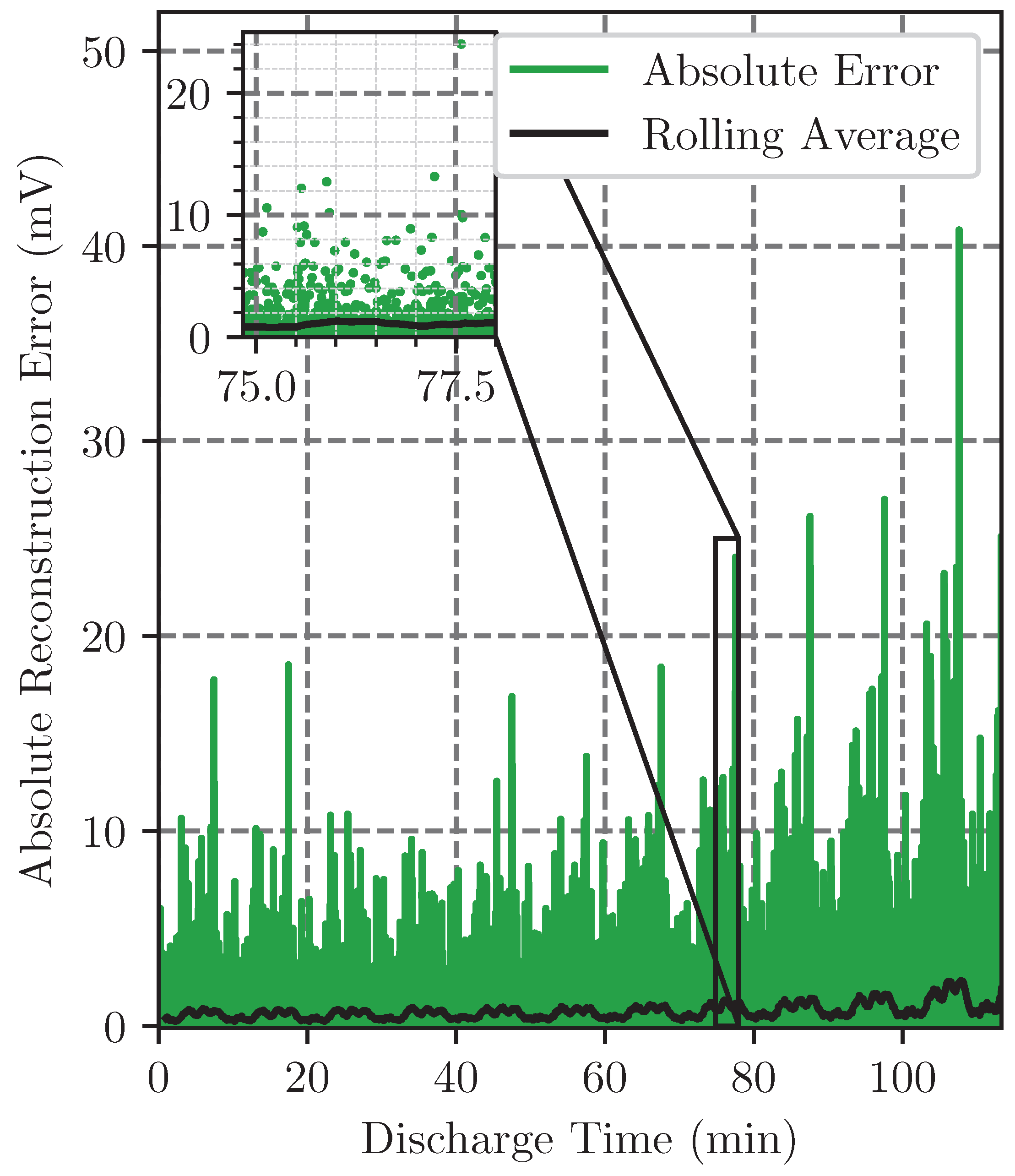
After evaluating the mean accuracy of the proposed compression method, Figure 11 shows the absolute error of reconstruction at each measurement in $\mathrm{m}$$\mathrm{V}$. The decompression of the US06 driving cycle at an ambient temperature of 25 °C with a RoC of 95% is used in this figure. A MAE of $1.57$ $\mathrm{m}$$\mathrm{V}$ and an RMSE of $2.75$ $\mathrm{m}$$\mathrm{V}$ are established. The figure shows each absolute errors of reconstruction in green. In black, the rolling average with a window size of 60 $\mathrm{s}$ is illustrated to visualize general changes in accuracy. When the error of reconstruction of each measurement is observed, a rise over discharge time can be seen. The zoom illustrated as a scatter plot shows that only some outliers with an error above 24 $\mathrm{m}$$\mathrm{V}$ can be observed. The zoom is chosen randomly. This observation can be punctuated by the rolling average with a window size of 60 $\mathrm{s}$ (black). A significant increase in the rolling average of the absolute reconstruction error can be seen after 6350 $\mathrm{s}$.

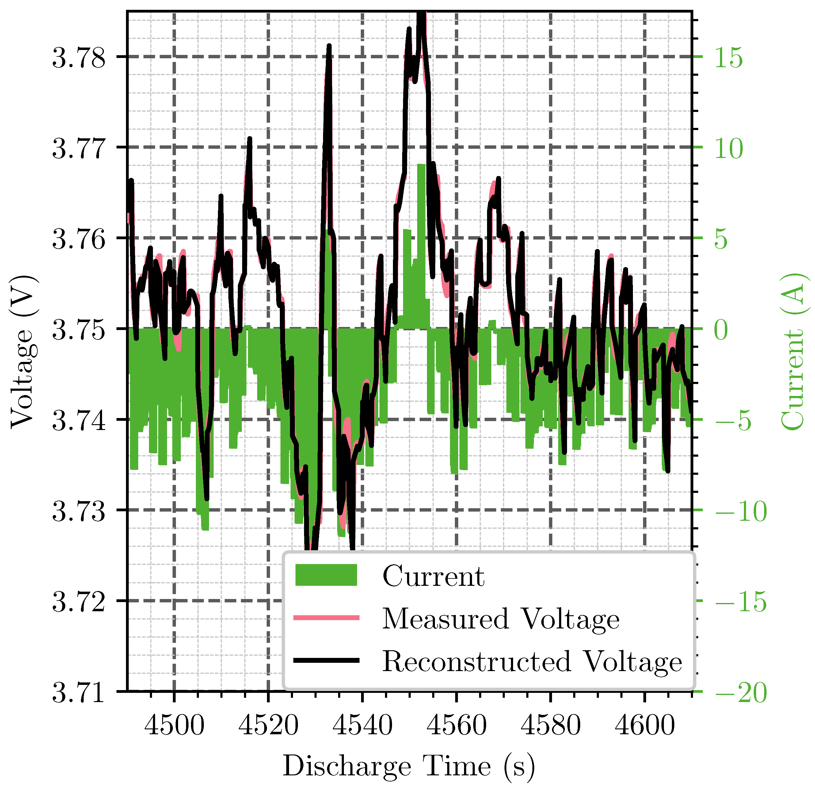
As already observed, the mean error during reconstruction is small, but many reconstructed measurements are outliers in mean error. To evaluate this, Figure 12 shows the measured voltage (orange) and reconstructed voltage (black), as well as the measured current (pink) for the zoom-in of Figure 11. This enables the conclusion that voltage peaks and dips cause the main outliers. This evaluation shows that, if high accuracy is necessary at voltage peaks and dips, this method shows weaknesses in reconstruction error. The maximum measured MAE/RMSE, as seen in Figure 9 and Figure 10, is 40 $\mathrm{m}$$\mathrm{V}$/62 $\mathrm{m}$$\mathrm{V}$ at a RoC of 99.75%, 14 $\mathrm{m}$$\mathrm{V}$/26 $\mathrm{m}$$\mathrm{V}$ at 95%, and 9 $\mathrm{m}$$\mathrm{V}$/16 $\mathrm{m}$$\mathrm{V}$ at 90% for the US06 drive cycle at an ambient temperature of $-10$ °C, which is significantly more accurate compared to the accuracy of the results proposed by Zhou et al. [17]. Zhou et al. specify an RMSE of $2.9$ $\mathrm{m}$$\mathrm{V}$, $4.16$ $\mathrm{m}$$\mathrm{V}$, and $10.01$ $\mathrm{m}$$\mathrm{V}$ at a RoC of 90%, 95%, and 99%. The highest precision could be measured with the HWFET drive cycle at an ambient temperature of 40 °C. For this drive cycle reconstruction, MAE and RMSE for 90%, 95%, and 99.75% can be observed at $0.01$ $\mathrm{m}$$\mathrm{V}$, $0.03$ $\mathrm{m}$$\mathrm{V}$, and $0.32$ $\mathrm{m}$$\mathrm{V}$.

3.2. Compression Runtime

In addition to accuracy, runtime is critical when implementing in real-world scenarios. For evaluation, the compression algorithm was implemented on an STM32L432 microcontroller with an Arm Cortex-M4 core at 80 $\mathrm{M}$$\mathrm{Hz}$. The experimental evaluation used, as input data, 10 $\min$ from the LA92 drive cycle data at 25 °C.

In Figure 13, the execution time per compression (green) and the approximated computation time for 600 data points (black) are illustrated. The measured execution time to compress 50 data points is $4.5$ $\mathrm{m}$$\mathrm{s}$. A linear increase in the execution time per time window of up to 35 $\mathrm{m}$$\mathrm{s}$ for 600 data points can be seen. These measurements lead to approximated runtimes per 600 compressed data points. For a window size of 50, the runtime is 54 $\mathrm{m}$$\mathrm{s}$. For 600 window sizes, the runtime is 35 $\mathrm{m}$$\mathrm{s}$. When integrated with the findings delineated in the preceding Section 3.1, it can be deduced that there exists an inverse relationship between computational speed and precision: a diminished execution time correlates with reduced accuracy, whereas an extended duration of computation enhances accuracy.

4. Conclusions and Outlook

The measurement and storage of the main attributes of a battery are one of the first initial steps to enable monitoring, digital twinning, and data-driven estimation methods for electrical vehicles. Therefore, efficient data compression and accurate decompression of measurements are required. This manuscript delineates a computationally efficient methodology for the lossy compression of voltage measurements. The salient points of the study are summarized as follows:

• Polynomial coding is used for voltage compression and reconstruction.
• The compression method exhibits notable computational efficiency, as evidenced by the experimental evaluation, which demonstrated an execution duration of merely 35 $\mathrm{m}$$\mathrm{s}$ to achieve a Rate of Compression (RoC) of 99.17%.
• The method exhibited suboptimal performance during cycles involving constant current conditions, and exhibited high accuracy under constant voltage and dynamic drive cycle conditions.
• The method established a MAE for a Rate of Compression of 99.75% between 16 $\mathrm{m}$$\mathrm{V}$ (UDDS) and 40 $\mathrm{m}$$\mathrm{V}$ (US06) with a measurement frequency of 10 $\mathrm{Hz}$ at the ambient temperature of $-10$ °C, $1.7$ $\mathrm{m}$$\mathrm{V}$ and $6.7$ $\mathrm{m}$$\mathrm{V}$ at 25 °C, and 1 $\mathrm{m}$$\mathrm{V}$ and 5 $\mathrm{m}$$\mathrm{V}$ at 40 °C.

The accuracy assessment of the CC-CV drive cycle has revealed the limitations of the proposed methodology when applied to compression data under constant current conditions. The experiments shown in Table 2 obtained a MAE of $2.4\pm 0.2$ to $27.9\pm 1.0$ $\mathrm{m}\mathrm{V}$. These results are comparable in accuracy with the results shown in Table 3 at an ambient temperature of $-10$ °C. It can, therefore, be concluded that, in addition to the temperature, the battery cells used also strongly influence the accuracy of the process. The results of the datasets discussed in Section 3.1.1 and Section 3.1.3 show this strong influence. However, the results indicate that the influence on the increase or decrease in accuracy depends on the battery and its chemistry. The reconstruction error correlates not only with RoC. It also depends significantly on the ambient temperature, as seen in Figure 10 and Table 3. Moreover, the accuracy in reconstruction shows that, for most of the used drive cycles, there is no significance in variation, and the drive cycles US06 and UDDS are outliers at this point.

To evaluate the model’s accuracy, it is also necessary to compare the results with the accuracy of the voltage sensors. In addition to the accuracy compared to the measurements from [33], the accuracy of BMSs and standards must also be considered. An accuracy of ± 2 $\mathrm{m}$$\mathrm{V}$ at 25 °C and $3.6$ $\mathrm{V}$ is specified for the Maximum Integrated Inc. MAX17843 Data-Acquisition Interface in the data sheet [35]. Texas Instruments lists 35 $\mathrm{m}$$\mathrm{V}$ as voltage measurement error in the reference design of EV/HEV Automotive Battery Monitoring [36]. This means that the evaluated MAE is, in some scenarios, lower than the expected sensor error.

Under some conditions, the method presented shows higher accuracies than the methods presented in the literature [17,18]. However, the method presented in this paper stands out due to its adaptive application. System-dependent parameters, such as the internal battery resistance, are not necessary. This represents a significant advantage in practical implementation.

Effective and accurate data compression is critical to real-time cloud-based digital twinning of battery packs and BMSs. This is caused by the bandwidth and storage requirements to stream and store the data. Lossy compression with compression rates as proposed in this paper of 99.75% per voltage measurement, in combination with the observed mean absolute reconstruction errors of maximum $4.0$ $\mathrm{m}$$\mathrm{V}$, can enable such technologies in research and science. Due to its low computational needs, this polynomial coding algorithm can be implemented in real-world BMS applications. The implementation in the STM32L432 microcontroller demonstrates this. A total execution time, ranging from 54 $\mathrm{m}$$\mathrm{s}$ to 35 $\mathrm{m}$$\mathrm{s}$, has been demonstrated during the compression of 600 data points at various compression rates.

To fully validate the method’s potential in real-world applications, future studies should evaluate its accuracy using real-time battery pack measurements from actual EV BMSs. This will provide valuable insights into its performance under dynamic operating conditions. Furthermore, the proposed lossy compression method has to be compared with other lossy, adaptive compression methods. Furthermore, investigating the possibility of incorporating time as an additional variable in the polynomial regression alongside the current could potentially enhance the method’s precision.